Geometric and projection effects in Kramers-Moyal analysis
Abstract
Kramers-Moyal coefficients provide a simple and easily visualized method with which to analyze stochastic time series, particularly nonlinear ones. One mechanism that can affect the estimation of the coefficients is geometric projection effects. For some biologically-inspired examples, these effects are predicted and explored with a non-stochastic projection operator method, and compared with direct numerical simulation of the systems’ Langevin equations. General features and characteristics are identified, and the utility of the Kramers-Moyal method discussed. Projections of a system are in general non-Markovian, but here the Kramers-Moyal method remains useful, and in any case the primary examples considered are found to be close to Markovian.
1 Introduction
In deterministic nonlinear systems, embedding theorems provide one method of reconstructing the system’s phase space and thereby obtaining a qualitative understanding, at least, of the system’s structure. In stochastic systems no such embedding theorems exist [1]. One approach for analyzing stochastic time series has been pioneered by Friedrich et al. [2, 3] and continues to be developed by Kleinhans [4, 5, 6] and others. The Kramers-Moyal coefficients (in one dimension),
| (1) |
are a critical part of the theory of Fokker-Planck equations, but only recently did Friedrich et al. suggest they could be computed directly from data. The first and second coefficients are known as the drift and diffusion coefficients; the higher-order coefficients are often zero [7]. The angle brackets denote an ensemble average, but if the Kramers-Moyal coefficient is constant in time this can be replaced with a time average. If the system can be modeled by a Langevin equation, or, equivalently, a Fokker-Planck equation, then the drift and diffusion coefficients completely characterize of the system.
Such an approach, already applied to fields including neuroscience [3], cardiology [8], traffic engineering [9], finance [10, 11] and turbulence [2], appears well suited to molecular biology, where biological structures commonly move in an overdamped, strongly Brownian environment [12]. Due to structural constraints, however, biological systems are often constrained in their motion to diffuse on a manifold which is no longer Cartesian. Experimentally, meanwhile, position measurements are usually taken in a Cartesian framework. Due to these geometrical effects the Kramers-Moyal coefficients derived from measurements are not the same as on the particle’s manifold. We show how these projected drift and diffusion coefficients can be used to make inferences about the original system’s dynamics.
For illustration, we consider three specific examples. Motivated by the diffusional search phase of myosin-V [13, 14] and other molecular motors, we consider a particle undergoing tethered diffusion with a rigid tether, so that the particle is constrained to a sphere. We assume its motion is recorded only in one linear dimension, with an experiment like the traveling wave tracking method of Cappello et al. [15] This involves the projection of a two-dimensional system onto one dimension. In this example, the diffusion on the sphere is free; in a second example, we make it harmonic in angle from a preferred orientation (‘biased diffusion on a sphere’). Lastly, we consider the more complicated example of a particle undergoing free diffusion on a sphere about a point itself undergoing biased diffusion on a sphere. We refer to this as ‘compound diffusion’.
We begin in section II with a simple example to illustrate the projection concept. After presenting a general framework for predicting geometrical effects in section III, we continue with the less trivial examples in sections IV and V. The effects of a non-Markovian projection are discussed in section VI, followed by conclusions in section VII.
2 Free diffusion on a sphere
Consider a particle diffusing on a sphere, of radius , under potential and constant local diffusion coefficient . Raible and Engel [16] found that the stochastic differential equations (SDEs, or Langevin equations) describing this motion in spherical polar co-ordinates are
| (2) | ||||
and are Wiener processes and the SDE is to be interpreted under the Itō convention. Setting for free diffusion and projecting onto , we have by the Itō rule for change of variables
| (3) |
This corresponds to drift and diffusion coefficients
| (4) | ||||
Therefore even though in local rectangular co-ordinates on the surface of the sphere the drift is zero and the diffusion constant (‘free diffusion’), in this projection the drift is linear, and the diffusion is an inverted (convex) parabola.
The drift coefficient is analogous to a position-dependent force, and the diffusion to a position-dependent temperature or ‘noise’ term [9]. Although the original motion on the surface was force-free with constant diffusion coefficient, we see the geometric projection introduces an effective ‘restoring force’, proportional to . It also introduces an effective noise which is maximal at but decreases to zero at : this prevents the projected particle from moving past the edge of the sphere.
The equilibrium probability distribution of this process is [7]
For free diffusion on a sphere, this gives a uniform distribution
| (5) |
This illustrates the power of the Kramers-Moyal approach. A naïve analysis of a stationary stochastic time series would be to construct its probability distribution. For the example above, this would give a uniform distribution, from which a reasonable guess for the system would be free diffusion in a one dimensional infinite potential well (corresponding to constant diffusion, and drift zero and infinite inside and at the edges of the well, respectively). On computing the drift and diffusion coefficients from a time series by Eq. (1), however, one would recover the drift and diffusion coefficients of Eqs. (4), and obtain a different characterization. One explanation of these drift and diffusion coefficients could be to recognize the system as a projection of free diffusion on a sphere, although this identification cannot be unique since we are projecting onto one dimension a two-dimensional system, and without a priori knowledge could be three- or higher-dimensional. Finally, if the projection is Markovian, as discussed below, the drift and diffusion coefficients fully characterize the dynamics in this co-ordinate, which the probability distribution does not.
Unlike stochastic autoregressive-type models [1], we see that the Kramers-Moyal approach permits arbitrary nonlinearity in the drift and diffusion coefficients to be recovered, and easily visualized.
3 General analysis of projections
Suppose we project the dynamics of a system onto some (collective) variable . Suppose the system can be written as a set of first-order stochastic differential equations. With the use of Itō’s chain rule, an SDE for in terms of may be derived,
| (6) |
We consider the estimation of the Kramers-Moyal coefficients (1) for this process. Writing the conditional expectation of Eq. (1) in an alternative form gives
where . We find , , and for [7]. But these coefficients still involve the full system variables , to which, we assume, the experiment does not have access.
From basic laws of conditional probability, it can be shown that the projection of these Kramers-Moyal coefficients from onto the subspace (which we distinguish from the unprojected coefficients by its arguments) is
| (7) |
This constitutes a projection operator for the Kramers-Moyal coefficients,
Clearly so is indeed a projection. As is a dynamical variable on the full phase space , the above coincides with the projection operator from the standard Zwanzig-Mori projection techniques [17]. To reiterate, however: before applying the projection operator to an arbitrary Langevin equation, one must transform the equation into the form of (6), one in the variable into which the system is to be projected. The quotient is also known as the conditional distribution for the subset of the full phase space distribution on the surface . The projection also has implications for the Markov property, as will be discussed in section 6.
If the 1-point densities and are well-defined, so are the projections (although they in some cases may be trivially zero). Furthermore, since for , then so do . The projected drift and diffusion coefficients, the equations above show, may be time-dependent even if the original system is homogeneous (the coefficients in its equations of motion independent of time) if the distribution is time-dependent (non-stationary). If the original system is both homogeneous and stationary, the projected drift and diffusion coefficients will be stationary.
The Kramers-Moyal coefficients may of course be computed directly from experimental data (1) of the projected variable. The necessary averages may be computed by time averaging if the projected drift and diffusion coefficients are stationary, which as just noted is when the full system is homogeneous and stationary. (This is in contrast to Kramers-Moyal analysis on the full system, where the system need only be homogeneous.) This projection operator method, however, provides a means of predicting the projected drift and diffusion coefficients from a model of the full system without the need for direct numerical simulation.
We now illustrate these observations with two examples.
4 Biased diffusion on a sphere
Suppose a particle is again undergoing diffusion on a sphere with local diffusion coefficient , but with a potential harmonic with angle away from a preferred binding direction. Align the -axis with this preferred direction so that . Substituting into the Langevin equations (2) for diffusion on a sphere, the equilibrium solution is
normalized such that .
Let us project this motion onto an axis tilted at angle from the -axis ( direction) in the plane,
| (8) |
The differential
| (9) |
can be calculated using Itō’s law for change of co-ordinates, and adding the noise terms, which we assume to be independent, in quadrature.
For the steady-state probability distribution as a function of , we calculate
the second equality by integrating over , and where we denote . The single integral that results we calculate numerically.
Similarly, from Eq. (7) we project the Kramers-Moyal coefficients by
| (10) |
where we have performed the integral over analytically, and in which is itself a function of .
In Fig. 1 we show drift and diffusion coefficients for computed from direct numerical simulation of Eqs. (2) and by the semi-analytical approach culminating in Eq. (10). The agreement between numerical and theoretical approaches is excellent, with two exceptions. At there are spikes due to the singularities in Eqs. (2). Raible and Engel [16] transform their equations into three-dimensional Cartesian co-ordinates before performing computations; we retain the spherical polar co-ordinates for transparency. Secondly, the larger binding potential for means the large negative regions of are poorly sampled and also may lead to finite sampling time effects [18].
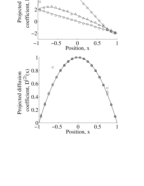
From Fig. 1 we see the potential on the sphere has an effect additional to the geometric effective force arising from the projection, and it is largest away from the potential minimum . The projected diffusion coefficients, meanwhile, show no change with the strength of the potential on the surface, . We infer that only the geometry of the system has affected the diffusion coefficient, and therefore that an inverted parabola shape for the diffusion coefficient is a good indicator of diffusion on a sphere.
More generally, if a particle is diffusing on a surface that is radially symmetric about the measurement axis , with radius , then the projected diffusion coefficient is independent of the potential on the surface. It can be shown from Raible and Engel’s formulas that the projected diffusion coefficient will be
assuming that the diffusion coefficient on the surface has constant value .
5 Compound diffusion on a sphere
We extend the previous scenario to one where there is a second rod undergoing tethered diffusion about the end of the first. We assume the first rod has a preferred binding angle, but that the second rod is diffusing freely. This models the motion of the unbound head during the diffusional search phase of molecular motors such as myosin-V.
In a first approximation, we assume that the motion of the end of the first rod with respect to its tethered end is given by the biased diffusion on a sphere of section IV, and the motion of the free end of the second rod with respect to the end joined to the first rod is given by the free diffusion on a sphere of section II. Once again we project onto a linear co-ordinate. The position of the end of the first rod is then from Eq. (8), and the end of the second rod , with given by Eq. (3) for . The equilibrium distribution of , is therefore given by Eq. (5). We further assume that the processes and are independent. Therefore the (unprojected) drift and diffusion coefficients are
We first require the equilibrium probability distribution for . Integrating over leaves the convolution
which can be computed numerically. For the drift and diffusion coefficients, from Eq. (7) we obtain, again after integrating over ,
Numerical results again together with semi-analytical predictions are shown in Fig. 2. Observe the unusual bimodal shape for the diffusion coefficient at , reflecting the two ‘spheres’ making up the diffusion process. As increases this shape begins changing towards a single inverted parabola which one would expect in the limit where the first rod is fixed. The drift is linear at . It maintains an approximately linear region but at larger develops large swings beyond , regions which will eventually become forbidden with a fixed first rod ().
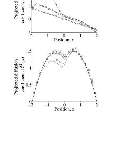
When the motor is in the diffusional search state, 1-D Kramers-Moyal analysis on experiments tracking the unbound head of myosin-V, or similar molecular motors, should (in the absence of other effects) give results like the above. Alternatively, if the marker is connected to a point on the unbound neck domain, the above simulations should be repeated with a shorter length for the second rod. Yildiz et al. [15] have performed such experiments on kinesin, from which they identified the step size and type (hand over hand), but their large sampling interval yields insufficient data for the present analysis.
6 Markov property
In our examples, the full system is Markov, that is, its next state depends only on the current one and not any other history:
where . Even if the full system is Markov, however, in general a projection is not [17]. Then the projected variable cannot be fully modeled by a Langevin equation (with history-independent coefficients), and so the drift and diffusion coefficients, or even all the Kramers-Moyal coefficients, cannot fully characterize the dynamics of the projected variables. Some authors [1] have criticized the Kramers-Moyal method on this basis, since experimentally one invariably can only access projections, not the entire system.
First, we wish to emphasize that even for projections that are demonstrably not Markovian, the Kramers-Moyal coefficients remain well-defined. In this case one may not write down an equation of motion of the system from the reconstructed coefficients, but they remain a useful tool for characterization and comparison of time series. Conversely, the existence of Kramers-Moyal coefficients, or 2-point probability densities, of course do not by themselves infer anything about the Markov property of the underlying process.
As an example of the Kramers-Moyal coefficients in a non-Markovian projection, consider the two-dimensional Ornstein-Uhlenbeck process
| (11) | ||||
projected onto . With a specific set of parameters, we plot the drift and diffusion coefficients in Fig. 3. As we will show below, this projection is non-Markovian. For this system the projection operation reduces to . Qualitatively, the projected drift and diffusion coefficients for a value of the projected variable are the values of the unprojected coefficients averaged by the likely locations of given this . In other words, they are the expectations over the conditional probability density . For this system we see in Fig. 3 an effective deterministic force tending to restore towards the origin, that is confine it to a finite region, and that there is a noise source operating directly on the variable.
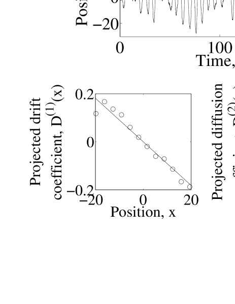
There are some cases where we know the projection will be Markovian. If the projected variable is slow compared to the other degrees of freedom of the system, the projection will be Markovian [17]. In the unbiased diffusion on a sphere of section 2 we saw that because of the special symmetry of the system, the second of the two degrees of freedom () was irrelevant for the projected variable, which by Eq. (3) we see is Markovian.
The Chapman-Kolmogorov equation [7]
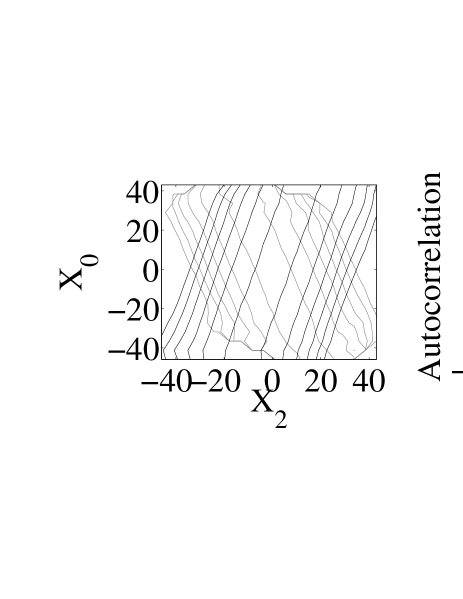
although not sufficient for the Markov property, is generally taken as a good test of it [10, 11, 20]. We tested the biased diffusion on a sphere of section 4 with the Chapman-Kolmogorov equation and the a posteriori test of Micheletti et al. [21]. Stationarity was assumed and the transition probabilities were calculated by time average, setting . The results are shown graphically in Figs. 4 and 5. These tests indicate that this projection of biased diffusion on a sphere is at least approximately Markovian. To a good approximation, then, the projected variable can be modeled by a Langevin equation in that variable, and in which the noise is Gaussian and delta-correlated.
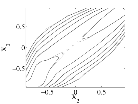
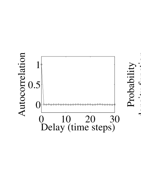
For comparison we show in Fig. 6 clear failure of the Chapman-Kolmogorov equation and Micheletti tests for a non-Markovian system, that of Eq. (11) projected onto .
7 Conclusions
We began with a simple example of projecting free diffusion on a sphere onto a rectangular co-ordinate. A general projector operator formalism for projecting Kramers-Moyal coefficients was then established. This was applied to biologically-inspired examples of biased diffusion on a sphere, and compound diffusion on a sphere, where excellent agreement with numerical results was observed. Generally speaking, the diffusion coefficient is more useful for identifying for the geometry of the surface on which the object is diffusing, the the drift coefficient for the potential on the surface. It was noted that the Kramers-Moyal coefficients can provide useful information even when the projection is not Markovian, which in general is the case, although the examples considered here were close to Markovian.
References
- [1] Holger Kantz and Thomas Schreiber. Nonlinear Time Series Analysis. Cambridge University Press, 2003.
- [2] R. Friedrich and J. Peinke. Description of a turbulent cascade by a Fokker-Planck equation. Phys. Rev. Lett., 78(5):863–866, Feb 1997.
- [3] R. Friedrich, S. Siegert, J. Peinke, St. Lück, M. Siefert, M. Lindemann, J. Raethjen, G. Deuschl, and G. Pfister. Extracting model equations from experimental data. Phys. Lett. A., 271:217–222, 2000.
- [4] D. Kleinhans and R. Friedrich. Maximum likelihood estimation of drift and diffusion functions. Phys. Lett. A, 368:194–198, 2007.
- [5] D. Kleinhans, R. Friedrich, A. Nawroth, and J. Peinke. An iterative procedure for the estimation of drift and diffusion coefficients of Langevin processes. Phys. Lett. A, 346(1-3):42–46, 2005.
- [6] David Kleinhans, Rudolf Friedrich, Matthias Wächter, and Joachim Peinke. Markov properties in presence of measurement noise. Phys. Rev. E, 76(4):041109, 2007.
- [7] H. Risken. The Fokker Planck Equation: Methods of Solution and Applications. Springer-Verlag, Berlin, 1984.
- [8] Tom Kuusela. Stochastic heart-rate model can reveal pathologic cardiac dynamics. Phys. Rev. E, 69(3):031916, Mar 2004.
- [9] S. Kriso, J. Peinke, R. Friedrich, and P. Wagner. Reconstruction of dynamical equations for traffic flow. Phys. Lett. A, 299(2-3):287–291, 2002.
- [10] R. Friedrich, J. Peinke, and Ch. Renner. How to quantify deterministic and random influences on the statistics of the foreign exchange market. Phys. Rev. Lett., 84(22):5224–5227, May 2000.
- [11] Fatemeh Ghasemi, Muhammad Sahimi, J. Peinke, R. Friedrich, G. Reza Jafari, and M. Reza Rahimi Tabar. Markov analysis and Kramers-Moyal expansion of nonstationary stochastic processes with application to the fluctuations in the oil price. Phys. Rev. E, 75(6):060102(R), 2007.
- [12] S. J. Lade, E. M. Craig, and H. Linke. Kramers-Moyal analysis of myosin-V walking data. in progress.
- [13] A. R. Dunn and J. A. Spudich. Dynamics of the unbound head during myosin V processive translocation. Nature Struct. Mol. Biol., 14:246–248, 2007.
- [14] Katsuyuki Shiroguchi and Kazuhiko Kinosita Jr. Myosin V walks by lever action and Brownian motion. Science, 316(5828):1208–1212, 2007.
- [15] G. Cappello, P. Pierobon, C. Symonds, L. Busoni, J. C. M. Gebhardt, M. Rief, and J. Prost. Myosin V stepping mechanism. Proc. Nat. Acad. Sci. USA, 104:15328–15333, 2007.
- [16] M. Raible and A. Engel. Langevin equation for the rotation of a magnetic particle. Appl. Organometal. Chem., 18:536–541, 2004.
- [17] R. Zwanzig. Nonequilibrium Statistical Mechanics. Oxford University Press, New York, 2001.
- [18] S. J. Lade. Finite sampling time effects in kramers-moyal analysis. submitted.
- [19] R. V. Erickson. Constant coefficient linear differential equations driven by white noise. Ann. Math. Stat., 42:820, 1971.
- [20] Mario Ragwitz and Holger Kantz. Indispensable finite time corrections for Fokker-Planck equations from time series data. Phys. Rev. Lett., 87(25):254501, Dec 2001.
- [21] C. Micheletti, G. Bussi, and A. Laio. Optimal Langevin modeling of out-of-equilibrium molecular dynamics simulations. J. Chem. Phys., 129:074105, 2008.