Analytical potential-density pairs from complex-shifted Kuzmin-Toomre discs

Abstract

The complex-shift method is applied to the Kuzmin-Toomre family of discs to generate a family of non-axisymmetric flat distributions of matter. These are then superposed to construct non-axisymmetric flat rings. We also consider triaxial potential-density pairs obtained from these non-axisymmetric flat systems by means of suitable transformations. The use of the imaginary part of complex-shifted potential-density pairs is also discussed.

Key words: galaxies: kinematics and dynamics.

1 Introduction

One of the difficulties encountered in modelling self-gravitating systems is set by the potential theory. In general, to calculate the gravitational potential associated with a matter distribution of arbitrary shape, one has to use numerical methods. On the other hand, it is convenient to have a set of analytical potential-density pairs that provide a description of gravitating systems, in particular, for those that deviate from spherical symmetry. A survey of such models can be found in [1], chapter 2.

A simple way to construct axisymmetric potential-density pairs that represent discs is the image method that is usually used to solve problems in electrostatics. This method was employed in the context of the Newtonian gravity first by Kuzmin [2], who derived a very simple potential-denstity pair of a disc (Section 3). Several years later, Evans & de Zeeuw [3] showed that any axisymmetric disc can be constructed by superposing simple Kuzmin discs with different weights. The image method has also been adapted to and used in General Relativity to generate several exact solutions of Einstein’s equations that represent discs (see e.g. [4, 5, 6, 7, 8, 9, 10, 11]).

Another technique to construct new solutions in the Newtonian gravity was introduced by Appell [12, 13] who considered the complexification of the potential of a point mass. This method, known as complex-shift method, was also used in General Relativity [14, 15, 16], but see some misinterpretations in the Appendix of [17]. More recently, the complex-shift method has been applied to spherical and axisymmetric Newtonian parent systems to generate new analytical axisymmetric and triaxial potential-density pairs [18, 19].

In this work, we use the complex-shift method to derive potential-dentity pairs for non-axisymmetric flat discs and rings and their “inflated” versions. In Section 2, we summarize the method of complexification. In Section 3, we complex shift the Kuzmin-Toomre family of discs to derive a family of non-axisymmetric flat discs. The members of this class are then superposed to generate further non-axisymmetric flat distributions of matter that can be interpreted as complex-shifted rings. This is done in Section 4. In Section 5, we use a general transformation to “inflate” the previous non-axisymmetric flat systems to generate triaxial potential-density pairs. We derive a generalized pair that includes an example studied by Ciotti & Marinacci [19]. In Section 6, we show that the imaginary part of a complex-shifted system can be superposed to another potential-density pair to generate physically acceptable systems which are not symmetrical with respect to a coordinate axis. At last, in Section 7 we summarize our results.

2 The complex-shift method

In this section, we briefly expose the idea of the complex-shift method. The formalism is similar to the presented by Ciotti & Giampieri [18] and Ciotti & Marinacci [19]. We start by considering a gravitational potential $\Phi(\mathbf{x})$ and an associated density distribution $\rho(\mathbf{x})$, where $\mathbf{x}=(x,y,z)$ is the position vector. We also assume that $\rho(\mathbf{x})$ satisfies the Poisson equation

$$\nabla^{2}\Phi=4\pi G\rho\mbox{.}$$ (1)

The basic idea of the complex-shift method is to obtain new potential-density pairs by a displacement of a given potential-density pair (the parent system) on the imaginary axis. The complexified potential is defined as $\Phi_{c}=\Phi(\mathbf{x}-i\mathbf{a})$, where $i$ is the imaginary unit and $\mathbf{a}$ is a real shift vector. Since the complex shift is a linear transformation and the Poisson equation is a linear partial differential equation (PDE) acting on the $\mathbf{x}$ vector, it follows that

$$\nabla^{2}\Phi_{c}=4\pi G\rho_{c}\mbox{,}$$ (2)

where $\rho_{c}=\rho(\mathbf{x}-i\mathbf{a})$ is the shifted mass density. By separating the real and imaginary parts of $\Phi_{c}$ and $\rho_{c}$, one obtains two real potential-density pairs.

Unfortunately, there is no guarantee that the resulting pairs describe physically acceptable (i.e. everywhere positive) gravitating systems. In fact, Ciotti & Giampieri [18] have shown that the imaginary part of the complex-shifted density always changes sign because the total mass of the complexified potential-density pair coincides with the total mass of the seed density distribution, and thus $\int\Im(\rho_{c})\mathrm{d}^{3}\mathbf{x}=0$. However, the real part can be positive everywhere. This usually happens for a finite domain of the shift vector $\mathbf{a}$.

3 Thin shifted Kuzmin-Toomre discs

In this Section, we apply the complex shift to the Kuzmin-Toomre family of discs [2, 20] to generate flat distributions of matter without axial symmetry. We begin with the first member of this family, which was the simple model derived by Kuzmin. The potential in the usual cylindrical coordinates $(R,z,\varphi)$ is given by

$$\Phi=-\frac{GM}{\sqrt{R^{2}+(b+|z|)^{2}}}\mbox{,}$$ (3)

where $b$ is a non-negative parameter. Using Poisson equation (1), the discontinuous normal derivative on $z=0$ introduces a surface density of mass

$$\sigma(R)=\frac{1}{2\pi G}\left.\frac{\partial\Phi}{\partial z}\right|_{z=0}\mbox{,}$$ (4)

which for the potential (3) results

$$\sigma(R)=\frac{bM}{2\pi\left(R^{2}+b^{2}\right)^{3/2}}\mbox{.}$$ (5)

The result of a complex shift of an axisymmetric potential depends not only on the length but also on the direction of the shift vector $\mathbf{a}$. We are interested in the equatorial shift of the potential (3), where without loss of generality we make a shift along the $x$-axis, $\mathbf{a}=(a,0,0)$. The complexified potential (3) reads

$$\Phi_{c}=-\frac{GM}{\sqrt{(x-ia)^{2}+y^{2}+(b+|z|)^{2}}}\mbox{.}$$ (6)

To evaluate the square root, we denote $d^{2}=x^{2}+y^{2}-a^{2}+(b+|z|)^{2}-2iax=u\mathrm{e}^{i\theta}$. Thus,

$$u=|d|^{2} =\sqrt{\left[x^{2}+y^{2}-a^{2}+(b+|z|)^{2}\right]^{2}+4a^{2}x^{2}}\mbox{,}$$ (7)

$$\cos\theta =\frac{x^{2}+y^{2}-a^{2}+(b+|z|)^{2}}{u},\qquad\sin\theta=-\frac{2ax}{u}\mbox{.}$$ (8)

For simplicity, we restrict to the case $\cos\theta>0$ everywhere, so we must have $a<b$. This restriction will be assumed henceforth. To make the square root a single valued function, we choose $d=\sqrt{u}\mathrm{e}^{i\theta/2}$, with

$$\cos\frac{\theta}{2}=\sqrt{\frac{1+\cos\theta}{2}},\qquad\sin\frac{\theta}{2}=\frac{\sin\theta}{2\cos(\theta/2)}\mbox{.}$$ (9)

With the help of equations (7)–(9), the real and imaginary parts of the potential (6) can be expressed as

$$\Re(\Phi_{c})=-\frac{GM}{\sqrt{2}}\sqrt{\frac{\chi+\sqrt{\chi^{2}+4a^{2}x^{2}}}{\chi^{2}+4a^{2}x^{2}}}\mbox{,}$$ (10)

$$\Im(\Phi_{c})=-\frac{\sqrt{2}GMax}{\sqrt{\chi^{2}+4a^{2}x^{2}}\sqrt{\chi+\sqrt{\chi^{2}+4a^{2}x^{2}}}}\mbox{,}$$ (11)

where $\chi=x^{2}+y^{2}-a^{2}+(b+|z|)^{2}$. The respective surface densities can be calculated using relation (4)

$$\Re(\sigma_{c})=\frac{Mb\sqrt{\xi+\sqrt{\xi^{2}+4a^{2}x^{2}}}}{2\sqrt{2}\pi\left(\xi^{2}+4a^{2}x^{2}\right)^{3/2}}\left(2\xi-\sqrt{\xi^{2}+4a^{2}x^{2}}\right)\mbox{,}$$ (12)

$$\Im(\sigma_{c})=\frac{Mabx\left(2\xi+\sqrt{\xi^{2}+4a^{2}x^{2}}\right)}{\sqrt{2}\pi\left(\xi^{2}+4a^{2}x^{2}\right)^{3/2}\sqrt{\xi+\sqrt{\xi^{2}+4a^{2}x^{2}}}}\mbox{,}$$ (13)

where we defined $\xi=x^{2}+y^{2}+b^{2}-a^{2}$. Equations (12) and (13) may also be obtained from the real and imaginary parts of the complexified surface density (5).

As was stated in Section 2, the imaginary part of the shifted Kuzmin-Toomre disc changes sign and becomes negative for $x<0$, so we focus on the real part. The expansion of the density (12) about the origin yields

$$\Re(\sigma_{c})\approx\frac{Mb}{2\pi(b^{2}-a^{2})^{3/2}}-\frac{3Mb(b^{2}+4a^{2})x^{2}}{4\pi(b^{2}-a^{2})^{7/2}}-\frac{3Mby^{2}}{4\pi(b^{2}-a^{2})^{5/2}}\mbox{.}$$ (14)

The isodensity curves are ellipses with major axis on the $y$-axis, minor-to-major squared axis ratio $(b^{2}-a^{2})/(b^{2}+4a^{2})$ and eccentricity $e=\sqrt{5a^{2}/(b^{2}+4a^{2})}$. Some curves of constant density in units of $M/b^{2}$ are displayed in Figs. 1(a) and (b) as functions of $x/b$ and $y/b$ for (a) $a/b=0.5$ and (b) $a/b=0.8$. We have a monotone decreasing surface density in the interval $0<a/b\lesssim 0.59$, whereas the density is always non-negative for $0<a/b\lesssim 0.86$. Expanding the potential (10) about the origin in the plane $z=0$ results

$$\Re(\Phi_{c})\approx-\frac{GM}{\sqrt{b^{2}-a^{2}}}+\frac{GM(b^{2}+2a^{2})x^{2}}{2(b^{2}-a^{2})^{5/2}}+\frac{GMy^{2}}{2(b^{2}-a^{2})^{3/2}}\mbox{,}$$ (15)

which is the potential of an anisotropic harmonic oscillator with the ratio of frequencies

$$\frac{\omega_{x}}{\omega_{y}}=\sqrt{\frac{b^{2}+2a^{2}}{b^{2}-a^{2}}}\mbox{.}$$ (16)

Therefore, we expect that test particles near the centre move in box orbits [1]. The contours in Fig. 1(b) suggest that the simple potential-density pair (10) and (12) may be used to represent thin galactic discs with a central bar.

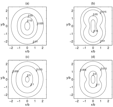
Figure 1: (a) and (b) Isodensity curves of the surface density (12) as functions of $x/b$ and $y/b$ for (a) $a/b=0.5$ and (b) $a/b=0.8$. (c) and (d) Isodensity curves of the surface density (20) as function of $x/b$ and $y/b$ for (b) $a/b=0.4$ and (b) $a/b=0.55$.

The potential-density pair obtained form the real part of the shifted Kuzmin-Toomre disc is in fact the first member of the family of non-axisymmetric thin disc-like structures. The other members can be calculated by using the recurrence relations for the Kuzmin-Toomre family of discs [21, 5]

$$\Phi_{c(n+1)}=\Phi_{c(n)}-\frac{b}{2n+1}\frac{\partial}{\partial b}\Phi_{c(n)}\mbox{,}$$ (17)

$$\sigma_{c(n+1)}=\sigma_{c(n)}-\frac{b}{2n+1}\frac{\partial}{\partial b}\sigma_{c(n)}\text{,}\qquad n=0,1,\ldots\mbox{,}$$ (18)

where $\Phi_{c(0)}$ and $\sigma_{c(0)}$ are given by equations (10) and (12), respectively. For instance, the potential and density of the next member read

$$\Phi_{c(1)}=-\frac{GM\sqrt{\chi+\sqrt{\chi^{2}+4a^{2}x^{2}}}}{\sqrt{2}\left(\chi^{2}+4a^{2}x^{2}\right)^{3/2}}\left[\chi^{2}+4a^{2}x^{2}\right.$$

$$\left.+b(b+|z|)\left(2\chi-\sqrt{\chi^{2}+4a^{2}x^{2}}\right)\right]\mbox{,}$$ (19)

$$\sigma_{c(1)}=\frac{3Mb^{3}\sqrt{\xi+\sqrt{\xi^{2}+4a^{2}x^{2}}}}{2\sqrt{2}\pi(\xi^{2}+4a^{2}x^{2})^{5/2}}\left(3\xi^{2}-2\xi\sqrt{\xi^{2}+4a^{2}x^{2}}-4a^{2}x^{2}\right)\mbox{,}$$ (20)

where $\chi=x^{2}+y^{2}-a^{2}+(b+|z|)^{2}$ and $\xi=x^{2}+y^{2}+b^{2}-a^{2}$. Some contours of the surface density (20) are shown in Figs. 1(c) and (d) as functions of $x/b$ and $y/b$ for shift parameters (a) $a/b=0.4$ and (b) $a/b=0.55$. Now a monotone decreasing density is found in the range $0<a/b\lesssim 0.44$, and a non-negative density in the interval $0<a/b\lesssim 0.58$.

4 Non-axisymmetric thin rings

We now use the family of non-axisymmetric thin discs discussed in the previous section to construct structures that can be considered as non-axisymmetric flat rings. The idea is to use superpositions of different members of the Kuzmin-Toomre family of discs to generate rings (zero mass density at the origin), as was done recently by Vogt & Letelier [22]. Let us briefly recall the main point of that work. The general expression for the surface density of the nth-order Kuzmin-Toomre disc is [21]

$$\sigma_{(n)}=\frac{(2n+1)b^{2n+1}M}{2\pi(R^{2}+b^{2})^{n+3/2}}\text{,}\qquad n=0,1,\ldots\mbox{,}$$ (21)

For convenience, we take discs with mass

$$M=\frac{2\pi b^{2}\sigma_{l}}{2n+1}\mbox{,}$$ (22)

where $\sigma_{l}$ is a constant with dimensions of surface density. Equation (21) is then rewritten as

$$\sigma_{(n)}=\frac{\sigma_{l}b^{2n+3}}{(R^{2}+b^{2})^{n+3/2}}=\frac{\sigma_{l}}{\left(1+R^{2}/b^{2}\right)^{n+3/2}}\mbox{.}$$ (23)

Now we consider the following superposition:

$$\sigma^{(m,n)}=\sum_{k=0}^{m}C^{m}_{k}(-1)^{m-k}\sigma_{(n+m-k)}\\ =\frac{\sigma_{l}}{\left(1+R^{2}/b^{2}\right)^{n+m+3/2}}\sum_{k=0}^{m}C^{m}_{k}(-1)^{m-k}\left(1+\frac{R^{2}}{b^{2}}\right)^{k}\mbox{,}$$ (24)

where $C^{m}_{k}=m!/[(m-k)!k!]$. Using

$$\sum_{k=0}^{m}C^{m}_{k}(-1)^{m-k}\left(1+\frac{R^{2}}{b^{2}}\right)^{k}=\left(\frac{R}{b}\right)^{2m}\mbox{,}$$ (25)

equation (24) takes the form

$$\sigma^{(m,n)}=\frac{\sigma_{l}\left(R/b\right)^{2m}}{\left(1+R^{2}/b^{2}\right)^{n+m+3/2}}\mbox{.}$$ (26)

We have that (26) with $m=1,2,\ldots$ and $n=0,1,\ldots$ defines a family of flat rings (characterized by zero density on $R=0$).

It would seem that a complexification of the density (26) would give rise to other ring structures. However, consider a shift $\sigma^{(m,n)}(x-ia)$ and evaluate the resulting complex density at the origin. We get

$$\sigma_{c}^{(m,n)}=\frac{\sigma_{l}(-1)^{m}\left(a/b\right)^{2m}}{\left(1-a^{2}/b^{2}\right)^{n+m+3/2}}\mbox{,}$$ (27)

which is non-zero and even negative when $m$ is odd. This indicates that in order to generate non-axisymmetric ring structures we should consider the superposition of complex-shifted Kuzmin-Toomre discs. We go back and apply a shift to equation (23), evaluate it at $(x=0,y=0)$,

$$\sigma_{c(n)}=\frac{\sigma_{l}}{\left(1-a^{2}/b^{2}\right)^{n+3/2}}\mbox{,}$$ (28)

and write the superposition

$$\sum_{k=0}^{m}\frac{\alpha_{k}\sigma_{l}}{\left(1-a^{2}/b^{2}\right)^{m-k+n+3/2}}=\frac{\sigma_{l}}{\left(1-a^{2}/b^{2}\right)^{m+n+3/2}}\sum_{k=0}^{m}\alpha_{k}\left(1-\frac{a^{2}}{b^{2}}\right)^{k}\mbox{.}$$ (29)

Now we impose the condition that the sum (29) be zero. Noting that

$$\sum_{k=0}^{m}C^{m}_{k}\left[-\left(1-\frac{a^{2}}{b^{2}}\right)\right]^{m-k}\left(1-\frac{a^{2}}{b^{2}}\right)^{k}=\left(-1+\frac{a^{2}}{b^{2}}+1-\frac{a^{2}}{b^{2}}\right)^{m}=0\mbox{,}$$ (30)

and comparing with (29), we get

$$\alpha_{k}=C^{m}_{k}(-1)^{m-k}\left(1-\frac{a^{2}}{b^{2}}\right)^{m-k}\mbox{.}$$ (31)

If we denote the surface density of the nth-order shifted Kuzmin-Toomre disc by $\sigma_{c(n)}$, then the superposition

$$\sigma_{c}^{(m,n)}=\sum_{k=0}^{m}C^{m}_{k}(-1)^{m-k}\left(1-\frac{a^{2}}{b^{2}}\right)^{m-k}\sigma_{c(n+m-k)}\mbox{,}$$ (32)

will be the equivalent to complex-shifted “rings” with zero surface density at the origin, and if $a=0$ the superposition reduces to the sum (24). The corresponding potential is calculated by a sum similar to (32). Note that the complex-shift of the family of rings given by (26) and the superposition of complex-shifted Kuzmin-Toomre discs given by (32) result in different structures, because the coefficients used in the sums are different.

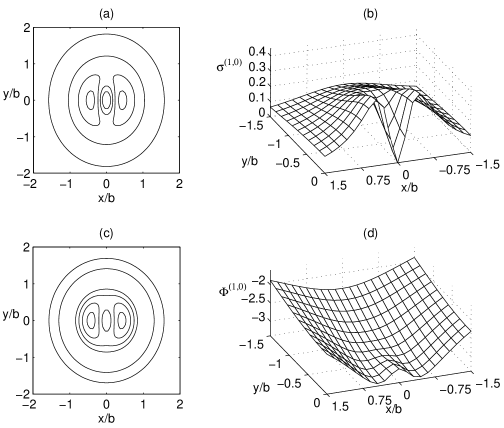
Figure 2: (a) and (b) Isodensity curves and surface plot of the surface density $\sigma_{c}^{(1,0)}/\sigma_{l}$ equation (34) with parameter $a/b=0.5$. (c) and (d) Isopotential curves and surface plot of the potential $\Phi_{c}^{(1,0)}/(\sigma_{l}Gb)$ (35) with parameter $a/b=0.5$.

As an example, we analyse the member with $m=1$, $n=0$

$$\sigma_{c}^{(1,0)}=\sigma_{c(0)}-\left(1-\frac{a^{2}}{b^{2}}\right)\sigma_{c(1)}\mbox{.}$$ (33)

Using equations (10), (12) and (19)–(20), the explicit expressions for the surface density and potential can be cast as

$$\sigma_{c}^{(1,0)}=\frac{\sigma_{l}b^{3}\sqrt{\xi+\sqrt{\xi^{2}+4a^{2}x^{2}}}}{\sqrt{2}(\xi^{2}+4a^{2}x^{2})^{5/2}}\left[\left(\xi^{2}+4a^{2}x^{2}\right)\left(2\xi-\sqrt{\xi^{2}+4a^{2}x^{2}}\right)\right.$$

$$\left.-(b^{2}-a^{2})\left(3\xi^{2}-2\xi\sqrt{\xi^{2}+4a^{2}x^{2}}-4a^{2}x^{2}\right)\right]\mbox{,}$$ (34)

$$\Phi_{c}^{(1,0)}=-\frac{2\pi\sigma_{l}Gb^{2}\sqrt{\chi+\sqrt{\chi^{2}+4a^{2}x^{2}}}}{3\sqrt{2}\left(\chi^{2}+4a^{2}x^{2}\right)^{3/2}}\left[\left(2+\frac{a^{2}}{b^{2}}\right)(\chi^{2}+4a^{2}x^{2})\right.$$

$$\left.-\left(1-\frac{a^{2}}{b^{2}}\right)b(b+|z|)\left(2\chi-\sqrt{\chi^{2}+4a^{2}x^{2}}\right)\right]\mbox{,}$$ (35)

where $\xi$ and $\chi$ were defined in Section 3. Near the centre, the approximate expressions for the potential-density pair are

$$\sigma_{c}^{(1,0)}\approx\frac{\sigma_{l}b^{3}(b^{2}+9a^{2})x^{2}}{(b^{2}-a^{2})^{7/2}}+\frac{\sigma_{l}b^{3}y^{2}}{(b^{2}-a^{2})^{5/2}}\mbox{,}$$ (36)

$$\Phi_{c}^{(1,0)}\approx-\frac{2\pi\sigma_{l}G(b^{2}+a^{2})}{3(b^{2}-a^{2})^{1/2}}-\frac{\pi\sigma_{l}G(b^{4}+7a^{2}b^{2}-2a^{4})x^{2}}{3(b^{2}-a^{2})^{5/2}}-\frac{\pi\sigma_{l}Gy^{2}}{3(b^{2}-a^{2})^{1/2}}\mbox{,}$$ (37)

which show that the density (potential) has a minimum (maximum) at the centre. Figs. 2(a)–(d) show level curves and surface plots of the dimensionless density $\sigma_{c}^{(1,0)}/\sigma_{l}$ and potential $\Phi_{c}^{(1,0)}/(\sigma_{l}Gb)$ with shift parameter $a/b=0.5$. Note that we do not have exactly a homogeneous mass concentration along a ring. Two points of maximum occur at $(x=\pm x_{s},y=0)$, where $x_{s}$ is the non-zero root of the equation $\partial\sigma_{c}^{(1,0)}/\partial x=0$ and has to be found numerically. Two saddle points also occur at $(x=0,y=\pm\sqrt{2(b^{2}-a^{2})/3})$. For $a/b=0.5$, we find $x_{s}/b\approx 0.43$ and saddle points at $y/b=\pm\sqrt{2}/2\approx\pm 0.71$. The potential shows two minimum points at $(x=\pm x_{p},y=0)$, where $x_{p}$ is the non-zero root of the equation $\partial\Phi_{c}^{(1,0)}/\partial x=0$, and two saddle points at $(x=0,y=\pm(b^{2}-a^{2})/\sqrt{a^{2}+2b^{2}})$. For $a/b=0.5$, we find $x_{p}/b\approx 0.42$ and saddle points at $y/b=\pm 1/2$.

The family of potential-density pairs derived in this Section may be useful to model ring galaxies, or R galaxies [23], objects in the form of approximate elliptical rings; in particular a subclass of such galaxies, designated RE galaxies, which have crisp, elliptical rings with photographically empty interiors.

5 Triaxial potential-density pairs from complex-shifted discs

The systems studied in previous sections were all flat, i.e., had infinitesimal thickness. One way to construct three-dimensional potential-density pairs from flat gravitating systems is to apply a transformation that involves the $z$-coordinate. For instance, Miyamoto & Nagai [24] proposed a transformation to “inflate” the thin Kuzmin-Toomre discs to obtain three-dimensional potential-density pairs for the disc part of galaxies. Other transformation based on a class of even polynomials was used by González & Letelier [10] and Vogt & Letelier [11] to generate thick General Relativistic discs.

We shall denote by $h(z)$ a general even function of the $z$-coordinate, and start with the real part of the potential of the complex-shifted Kuzmin-Toomre disc, where we replace $|z|$ by $h(z)$

$$\Re(\Phi_{c})=-\frac{GM}{\sqrt{2}}\sqrt{\frac{\zeta+\sqrt{\zeta^{2}+4a^{2}x^{2}}}{\zeta^{2}+4a^{2}x^{2}}}\mbox{,}$$ (38)

where now we define $\zeta=x^{2}+y^{2}-a^{2}+[b+h(z)]^{2}$. The resulting mass density follows directly from Poisson equation (1) in the usual Cartesian coordinates. We obtain

$$\rho_{c(0)}=\frac{M(b+h)h_{,zz}\sqrt{\zeta+\sqrt{\zeta^{2}+4a^{2}x^{2}}}}{4\sqrt{2}\pi\left(\zeta^{2}+4a^{2}x^{2}\right)^{3/2}}\left(2\zeta-\sqrt{\zeta^{2}+4a^{2}x^{2}}\right)\\ +\frac{M\left(1-h_{,z}^{2}\right)\sqrt{\zeta+\sqrt{\zeta^{2}+4a^{2}x^{2}}}}{4\sqrt{2}\pi\left(\zeta^{2}+4a^{2}x^{2}\right)^{5/2}}\left[3(b+h)^{2}\right.\\ \left.\times\left(3\zeta^{2}-2\zeta\sqrt{\zeta^{2}+4a^{2}x^{2}}-4a^{2}x^{2}\right)-\left(\zeta^{2}+4a^{2}x^{2}\right)\left(2\zeta-\sqrt{\zeta^{2}+4a^{2}x^{2}}\right)\right]\mbox{.}$$ (39)

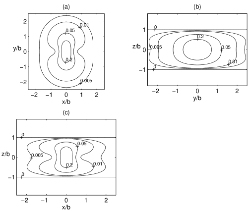
Figure 3: Isodensity curves of the mass density $\rho_{c(0)}/(M/b^{3})$ equation (39) in the three orthogonal coordinate planes for the polynomial class of functions (40). Parameters: $a/b=0.6$, $n=1$, $w=0$ and $s/b=1$.

Note that to satisfy the restriction $\cos\theta>0$ in (8), we must have $\zeta>0$ everywhere. In the case of a Miyamoto & Nagai transformation [24], $h(z)=\sqrt{z^{2}+c^{2}}$ with $c>0$, and the potential-density pair (38) and (39) is the same as studied by Ciotti & Marinacci [19], who performed an equatorial shift of the Miyamoto-Nagai disc. We can also use the class of polynomials used in [10, 11]

$$h(z)=\begin{cases}-z+C,&z\leq-s,\\ Az^{2}+Bz^{2n+2},&-s\leq z\leq s,\\ z+C,&z\geq s,\end{cases}$$ (40)

where

$$A=\frac{2n+1-sw}{4ns},\quad B=\frac{sw-1}{4n(n+1)s^{2n+1}},\quad C=-\frac{s(2n+1+sw)}{4(n+1)},$$ (41)

with $n=1,2,\ldots$; $s$ is the half-thickness of the disc and $w$ is the jump of $h_{,zz}$ on $z=\pm s$. For $|z|>s$, we have $h_{,z}=\pm 1$ and $h_{,zz}=0$, so there is no matter in this region. We will consider the special case $w=0$, so $h_{,zz}(z=\pm s)=0$ and the density also vanishes there. Figs. 3(a)–(c) show isodensity curves in the three orthogonal coordinate planes of the mass density $\rho_{c(0)}/(M/b^{3})$ for the polynomial with $n=1$, half-thickness $s/b=1$ and shift parameter $a/b=0.6$. We find that the mass density is non-negative in the range $0<a/b\lesssim 0.62$, and when the half-thickness is reduced to $s/b=0.5$ the interval becomes $0<a/b\lesssim 0.70$. The main qualitative difference between our system and the one studied by Ciotti & Marinacci [19] for the Miyamoto-Nagai shifted disc lies in the finite thickness of the former.

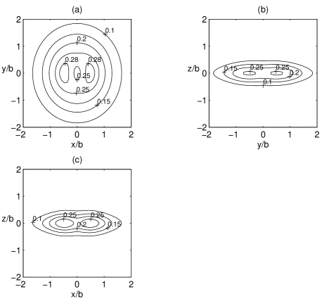
Figure 4: Isodensity curves in the three orthogonal coordinate planes of the surface density $\rho_{c}^{(1,0)}/(\sigma_{l}/b)$ equation (42) for shift parameter $a/b=0.5$ and a Miyamoto-Nagai transformation with parameter $c/b=0.5$.

The “inflated” version of the ring-like non-axisymmetric flat systems (34) and (35) also can be found by replacing $|z|$ by $h(z)$ in the potential (35) and calculating the resulting mass density with Poisson equation. One ends with

$$\rho_{c}^{(1,0)}=\frac{\sigma_{l}b^{2}h_{,zz}\sqrt{\zeta+\sqrt{\zeta^{2}+4a^{2}x^{2}}}}{6\sqrt{2}\left(\zeta^{2}+4a^{2}x^{2}\right)^{5/2}}\left\{\left[3b+h(2+a^{2}/b^{2})\right]\left(\zeta^{2}+4a^{2}x^{2}\right)\right.\\ \left.\times\left(2\zeta-\sqrt{\zeta^{2}+4a^{2}x^{2}}\right)-3b(b+h)^{2}(1-a^{2}/b^{2})\left(3\zeta^{2}-2\zeta\sqrt{\zeta^{2}+4a^{2}x^{2}}-4a^{2}x^{2}\right)\right\}\\ +\frac{\sigma_{l}b^{2}\left(1-h_{,z}^{2}\right)\sqrt{\zeta+\sqrt{\zeta^{2}+4a^{2}x^{2}}}}{6\sqrt{2}\left(\zeta^{2}+4a^{2}x^{2}\right)^{7/2}}\left\{3(b+h)\left[5b+2h+(h-2b)a^{2}/b^{2}\right]\right.\\ \left.\times\left(\zeta^{2}+4a^{2}x^{2}\right)\left(3\zeta^{2}-2\zeta\sqrt{\zeta^{2}+4a^{2}x^{2}}-4a^{2}x^{2}\right)-15b(b+h)^{3}(1-a^{2}/b^{2})\right.\\ \left.\times\left(4\zeta^{3}-3\zeta^{2}\sqrt{\zeta^{2}+4a^{2}x^{2}}+4a^{2}x^{2}\sqrt{\zeta^{2}+4a^{2}x^{2}}-16\zeta a^{2}x^{2}\right)\right.\\ \left.-(2+a^{2}/b^{2})\left(\zeta^{2}+4a^{2}x^{2}\right)^{2}\left(2\zeta-\sqrt{\zeta^{2}+4a^{2}x^{2}}\right)\right\}\mbox{.}$$ (42)

Some isodensity curves in the three orthogonal coordinate planes of the mass density $\rho_{c}^{(1,0)}/(\sigma_{l}/b)$ are shown in Figs. 4(a)–(c), for the case of a Miyamoto-Nagai transformation $h(z)=\sqrt{z^{2}+c^{2}}$. The values of the parameters used were $a/b=0.5$ and $c/b=0.5$. As expected, one has a non-axisymmetric toroidal mass distribution.

6 Using the imaginary part of complex-shifted discs

In Section 2, we commented that the imaginary part of a complex-shifted density always changes sign [18], and therefore is not adequate for modelling gravitating systems. In fact, the imaginary part of the shifted Kuzmin-Toomre disc (13) is negative for $x<0$. Figs. 5(a) and (b) display level curves and the surface plot of the imaginary part of the dimensionless surface density with shift parameter $a/b=0.5$.

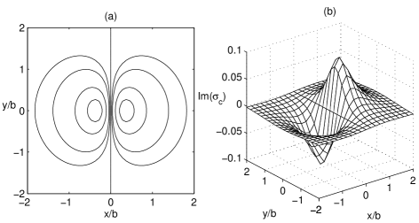
Figure 5: (a) Isodensity curves and (b) surface plot of the surface density $\Im(\sigma_{c})/(M/b^{2})$ equation (13) with shift parameter $a/b=0.5$.

Now the combination of the imaginary part of a complex-shifted system with another potential-density pair may generate well-behaved and interesting new configurations. To illustrate our point, we take the superposition of the real and the imaginary part of the complex-shifted Kuzmin disc (6)

$$\sigma_{sup.}=\Re(\sigma_{c})+\beta\Im(\sigma_{c})\mbox{,}$$ (43)

where $\beta$ is a dimensionless parameter which we assume positive, and an analogous expression holds for the potential. We have chosen this example for its simplicity, but in principle the superposition does not need to involve the real and imaginary parts of the same shifted system. Using equations (10)–(13), we obtain

$$\Phi_{sup.}=-\frac{GM\left(\chi+\sqrt{\chi^{2}+4a^{2}x^{2}}+2\beta ax\right)}{\sqrt{2}\sqrt{\chi^{2}+4a^{2}x^{2}}\sqrt{\chi+\sqrt{\chi^{2}+4a^{2}x^{2}}}}\mbox{,}$$ (44)

$$\sigma_{sup.}=\frac{Mb}{2\sqrt{2}\pi\left(\xi^{2}+4a^{2}x^{2}\right)^{3/2}\sqrt{\xi+\sqrt{\xi^{2}+4a^{2}x^{2}}}}\left[\left(\xi+\sqrt{\xi^{2}+4a^{2}x^{2}}\right)\right.$$

$$\left.\times\left(2\xi-\sqrt{\xi^{2}+4a^{2}x^{2}}\right)+2\beta ax\left(2\xi+\sqrt{\xi^{2}+4a^{2}x^{2}}\right)\right]\mbox{.}$$ (45)

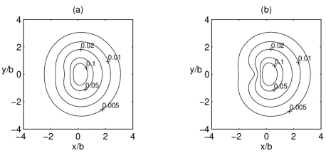
Figure 6: Isodensity curves of the surface density $\sigma_{sup.}/(M/b^{2})$ equation (45) for shift parameter $a/b=0.5$ and (a) $\beta=0.5$, (b) $\beta=0.8$.

Isodensity curves of (45) are shown in Figs. 6(a) and (b) for shift parameter $a/b=0.5$, $\beta=0.5$ in Fig. 6(a) and $\beta=0.8$ in Fig. 6(b). The mass distribution is no more symmetric with respect to the $x=0$ axis. For $x>0$, the imaginary part of the shifted density adds mass to the real part, and when $x<0$ there is a subtraction of mass. The maximum of density is displaced from the centre along the $x$-axis; in the examples shown in Fig. 6(a) the maximum is located at $x/b\approx 0.09$ and in Fig. 6(b) at $x/b\approx 0.13$. For the values of $\beta$ shown in Figs. 6(a) and (b), the surface density is non-negative everywhere, but one can expect that if $\beta$ becomes too large regions with negative densities should appear. In fact, we find the following intervals of $\beta$, depending on the shift parameter, where the superposed density is non-negative: for $a/b=0.25$, $0<\beta\lesssim 2.5$; for $a/b=0.5$, $0<\beta\lesssim 1.0$; and for $a/b=0.75$, $0<\beta\lesssim 0.3$.

It is also possible to “inflate” the flat potential-density pair (44) and (45) by using the same procedure described in Section 5. One obtains the following result:

$$\Phi_{sup.}=-\frac{GM\left(\zeta+\sqrt{\zeta^{2}+4a^{2}x^{2}}+2\beta ax\right)}{\sqrt{2}\sqrt{\zeta^{2}+4a^{2}x^{2}}\sqrt{\zeta+\sqrt{\zeta^{2}+4a^{2}x^{2}}}}\mbox{,}$$ (46)

$$\rho_{sup.}=\frac{M(b+h)h_{,zz}}{4\sqrt{2}\pi\left(\zeta^{2}+4a^{2}x^{2}\right)^{3/2}\sqrt{\zeta+\sqrt{\zeta^{2}+4a^{2}x^{2}}}}\left[\left(\zeta+\sqrt{\zeta^{2}+4a^{2}x^{2}}\right)\right.$$

$$\left.\times\left(2\zeta-\sqrt{\zeta^{2}+4a^{2}x^{2}}\right)+2\beta ax\left(2\zeta+\sqrt{\zeta^{2}+4a^{2}x^{2}}\right)\right]$$

$$+\frac{M\left(1-h_{,z}^{2}\right)}{4\sqrt{2}\pi\left(\zeta^{2}+4a^{2}x^{2}\right)^{5/2}\sqrt{\zeta+\sqrt{\zeta^{2}+4a^{2}x^{2}}}}\left\{-\left(\zeta^{2}+4a^{2}x^{2}\right)\right.$$

$$\left.\times\left[\left(\zeta+\sqrt{\zeta^{2}+4a^{2}x^{2}}\right)\left(2\zeta-\sqrt{\zeta^{2}+4a^{2}x^{2}}\right)+2\beta ax\left(2\zeta+\sqrt{\zeta^{2}+4a^{2}x^{2}}\right)\right]\right.$$

$$\left.+3(b+h)^{2}\left[\left(\zeta+\sqrt{\zeta^{2}+4a^{2}x^{2}}\right)\left(3\zeta^{2}-2\zeta\sqrt{\zeta^{2}+4a^{2}x^{2}}-4a^{2}x^{2}\right)\right.\right.$$

$$\left.\left.+2\beta ax\left(3\zeta^{2}+2\zeta\sqrt{\zeta^{2}+4a^{2}x^{2}}-4a^{2}x^{2}\right)\right]\right\}\mbox{,}$$ (47)

where, as before, $\zeta=x^{2}+y^{2}-a^{2}+[b+h(z)]^{2}$. As an example we take $h(z)=\sqrt{z^{2}+c^{2}}$. Figs. 7(a)–(c) show isodensity curves of the mass density $\rho_{sup.}/(M/b^{3})$ on the three orthogonal coordinate planes for parameters $a/b=0.5$, $\beta=0.8$ and $c/b=0.3$. In Figs. 7(b) and (c), the values of the level curves are the same as indicated in Fig. 7(a). Again the lack of symmetry with respect to the $x=0$ axis is noted.

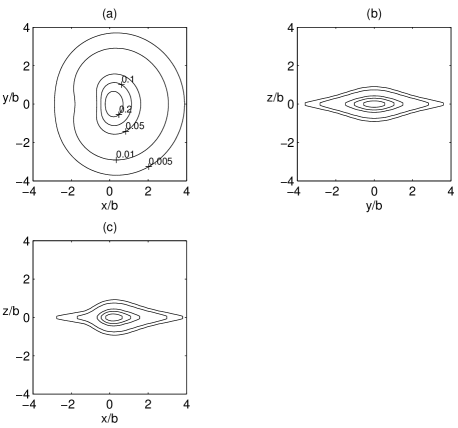
Figure 7: Isodensity curves in the three orthogonal coordinate planes of the surface density $\rho_{sup.}/(M/b^{3})$ equation (47) for parameters $a/b=0.5$, $\beta=0.8$ and a Miyamoto-Nagai transformation with parameter $c/b=0.3$.

7 Discussion

The method of complexification, also known as complex-shift method, was used to generate a family of non-axisymmetric flat discs using the Kuzmin-Toomre family of discs as the parent system. The discs present non-negative surface densities for restricted ranges of the shift parameter. Further we showed how these discs can be superposed to yield non-axisymmetric structures with vanishing surface density at the origin that can be considered as complex-shifted flat rings. We also “inflated” the aforementioned flat potential-density pairs by a general transformation and presented some examples by using a Miyamoto-Nagai transformation and a class of polynomials. These resulted in triaxial potential-density pairs. We also showed that the imaginary part of a complex-shifted system, which has non-physical characteristics, can be combined with other pairs to generate well-behaved systems that are not symmetrical with respect to a coordinate axis.

The analytical potential-density pairs presented in this work can all be expressed in terms of elementary functions, and yet show non-trivial features. We hope they may be useful as more realistic models in galactic dynamics.

References

- [1] Binney J., Tremaine S., 2008, Galactic Dynamics, 2nd edn. Princeton Univ. Press, Princeton, NJ
- [2] Kuzmin G.G., 1956, Astron. Zh., 33, 27
- [3] Evans N.W., de Zeeuw P.T., 1992, MNRAS, 257, 152
- [4] Bičák J., Lynden-Bell D., Katz J., 1992, Phys. Rev. D, 47, 4334
- [5] Bičák J., Lynden-Bell D., Pichon C., 1993, MNRAS, 265, 126
- [6] Ledvinka T., Zofka M., Bičák J., 1999, in Piran T., ed., Proc. 8th Marcel Grossman Meeting in General Relativity, World Scientific, Singapore, p. 339-341.
- [7] Letelier P.S, 1999, Phys. Rev. D, 60, 104042
- [8] González G.A., Letelier P.S., 2000, Phys. Rev. D, 62, 064025
- [9] Vogt D., Letelier P.S., 2003, Phys. Rev. D, 68, 084010
- [10] González G.A., Letelier P.S., 2004, Phys. Rev. D, 69, 044013
- [11] Vogt D., Letelier P.S., 2005, Phys. Rev. D, 71, 084030
- [12] Appell P., 1887, Ann. Math. Lpz., 30, 155
- [13] Whittaker E.T., Watson G.N., 1950, A Course of Modern Analysis. Cambridge Univ. Press, Cambridge
- [14] Letelier P.S, Oliveira S.R., 1987, J. Math. Phys., 28, 165
- [15] Gleiser R.J., Pullin J.A., 1989, Class. Quantum Gravity, 6, 977
- [16] Letelier P.S, Oliveira S.R., 1998, Class. Quantum Gravity, 15, 421
- [17] D’Afonseca L.A., Letelier P.S, Oliveira S.R., 2005, Class. Quantum Gravity, 22, 3803
- [18] Ciotti L., Giampieri G., 2007, MNRAS, 376, 1162
- [19] Ciotti L., Marinacci F., 2008, MNRAS, 387, 1117
- [20] Toomre A., 1963, ApJ, 138, 385
- [21] Nagai R., Miyamoto M., 1976, PASJ, 28, 1
- [22] Vogt D., Letelier P.S., 2009, MNRAS, 396, 1487
- [23] Theys J.C., Spiegel E.A., 1976, ApJ, 208, 650
- [24] Miyamoto M., Nagai R., 1975, PASJ, 27, 533