Coupled Modulated Bilayers

Abstract

We propose a model addressing the coupling mechanism between two spatially modulated monolayers. We obtain the mean-field phase diagrams of coupled bilayers when the two monolayers have the same preferred modulation wavelength. Various combinations of the monolayer modulated phases are obtained and their relative stability is calculated. Due to the coupling, a spatial modulation in one of the monolayers induces a similar periodic structure in the second one. We have also performed numerical simulations for the case when the two monolayers have different modulation wavelengths. Complex patterns may arise from the frustration between the two incommensurate but annealed structures.

I Introduction

Quite a number of physical, chemical, and biological systems manifest some type of modulation in their spatial ordering SA ; AR1 ; AR2 . Such structures are stripes and bubbles in two-dimensional (2D) systems, or lamellae, hexagonally packed cylinders, and cubic arrays of spheres in three-dimensional (3D) cases as well as more complex structures such as gyroids. Examples of such systems include ferromagnetic layers DBBEGHJOPPT , magnetic garnet films GD , ferrofluids AR1 ; AR2 ; Rosensweig , dipolar Langmuir films ABJ , rippled phases in lipid bilayers Sackmann1 , and block copolymers Hamley ; Fredrickson . Modulated phases may also occur in systems described by two (or more) coupled order parameters, each favoring a different equilibrium state LA . The observed spatial patterns exhibit striking similarity even for systems that are very different in their nature. It is generally understood that the modulated structures are formed spontaneously due to the competition between short- and long-range interactions.

In the case of 2D ferromagnetic layers, for example, the short-range interaction arises from magnetic domain wall energy, while the long-range interaction is due to magnetic dipole-dipole interaction which induces a demagnetizing field AR1 ; AR2 . Adding both contributions and minimizing the total free energy with respect to the wavenumber $q$, one obtains the most stable mode $q^{\ast}\neq 0$. This description is valid in the weak segregation limit (close to a critical point), where the equilibrium domain size is given by $d^{\ast}=2\pi/q^{\ast}$. In general, this quantity depends on temperature and/or other external fields.

In this paper, we shall consider two modulated monolayers that are jointly coupled. Our motivation is related to recent experiments by Collins and Keller CK who investigated Montal-Mueller planar bilayer membranes MM composed of lipids and cholesterol. In this technique, a bilayer is constructed by preparing separately two independent monolayers and then combining them into one joint bilayer across a hole at the air/water interface. The experiments addressed specifically the question of liquid domains in the two leaflets, and the mutual influence of the monolayers in terms of their domain phases. In the experiment, asymmetric bilayers are prepared in such a way that one leaflet’s composition would phase-separate in a symmetric bilayer and the other’s would not. In some cases, one leaflet may induce phase separation in the other leaflet, whereas in other cases, the second leaflet suppresses domain formation in the original leaflet. These results imply that the two leaflet coupling is important ingredient in determining the bilayer phase state.

Motivated by these experiments, the coupled bilayer system was investigated theoretically. The coupling mechanism arises through interactions between lipid tails across the bilayer midplane, and the phase behavior of such a bilayer membrane was computed using either regular solution theory WLM or Landau theory PS . The theoretical results are in accord with several of the experimental observations. It should be noted that all previous models dealt with the coupling between two macro–phase separated leaflets, while it is also of interest to investigate the coupling between two micro–phase separated (modulated) leaflets. Furthermore, one might also consider the interplay between a macro– and a micro–phase separation.

In the present work, we suggest a model describing the coupling between two modulated systems, and, in particular, we analyze the influence of this coupling on the phase behavior of two coupled 2D monolayers. When the two monolayers have the same preferred periodicity of modulation, we obtain the mean-field phase diagrams which exhibit various combinations of micro–phase separated structures. In some cases, the periodic structure in one of the monolayers will induce a modulation in the other monolayer. Interesting situations take place when the two monolayers have different preferred wavelengths of modulation. Here the frustrations between the two competing modulated structures need to be optimized. These structures and their dynamical behavior are examined using numerical simulations. Although there has been so far no experiment which directly corresponds to the proposed model, our predictions may be verified, for example, by constructing Montal-Mueller bilayers MM out of two lipid monolayers that exhibit a striped phase near the miscibility critical point KPHM ; KM .

In the next section, we present a phenomenological model describing the coupling between two modulated lipid monolayers. In Sec. III, we discuss the case when the two monolayers have the same preferred wavelength of modulation. Monolayers having different preferred wavelengths will be considered in Sec. IV, and some related situations are further discussed in Sec. V. Although we limit our present analysis to 2D systems, the suggested model can be generalized to 3D systems as well.

II Model

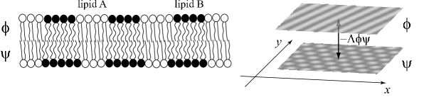
Figure 1: Schematic illustration of two coupled modulated monolayers forming a bilayer membrane. Each monolayer is composed of a binary A/B lipid mixture, which can have a spatial modulation. The relative composition of the two lipids in the upper and the lower leaflets are defined by $\phi$ and $\psi$, respectively. In general, the average composition in the two monolayers can be different. The lipid tails interact across the bilayer midplane. The phenomenological coupling term between these two variables are assumed to be bilinear of the form ${-}\Lambda\phi\psi$ in the free energy of Eq. (1).

In order to illustrate the coupling effect between two modulated systems, we imagine a pair of lipid monolayers forming a coupled bilayer. Each of the monolayer can undergo separately a micro–phase separation. As shown in Fig. 1, we assume that each monolayer is a mixture of two lipid species, say lipid A and lipid B. Their area fractions are defined by $\phi_{\rm A}(\mathbf{r})$ and $\phi_{\rm B}(\mathbf{r})$, where $\mathbf{r}=(x,y)$ is the 2D positional vector. By assuming that the monolayer is incompressible, $\phi_{\rm A}(\mathbf{r})+\phi_{\rm B}(\mathbf{r})=1$, the monolayer composition can be characterized by a single order parameter defined by the relative A/B composition $\phi(\mathbf{r})=\phi_{\rm A}(\mathbf{r})-\phi_{\rm B}(\mathbf{r})$. Let us denote this local order parameter of the upper and lower monolayers by $\phi(\mathbf{r})$ and $\psi(\mathbf{r})$, respectively. The coarse-grained free-energy functional for the coupled modulated bilayer is written as:

$$F[\phi,\psi] =F_{\rm u}[\phi]+F_{\rm\ell}[\psi]-\Lambda\int{\rm d}\mathbf{r}\,\phi\psi$$

$$=\int{\rm d}\mathbf{r}\biggl{[}2(\nabla^{2}\phi)^{2}-2(\nabla\phi)^{2}+\frac{\tau}{2}\phi^{2}+\frac{1}{4}\phi^{4}-\mu_{\phi}\phi$$

$$+2D(\nabla^{2}\psi)^{2}-2C(\nabla\psi)^{2}+\frac{\tau}{2}\psi^{2}+\frac{1}{4}\psi^{4}-\mu_{\psi}\psi-\Lambda\phi\psi\biggr{]}.$$ (1)

This is a modified Ginzburg-Landau free energy expanded in powers of the order parameters $\phi$ and $\psi$ and their derivatives. The $F_{\rm u}[\phi]$ free energy has five terms depending only on $\phi$ and its derivatives. It describes the upper monolayer and its possible modulations, while the coefficients of the Laplacian squared, the gradient squared and the $\phi^{4}$ terms are taken to be numbers, for simplicity. Similarly, $F_{\rm\ell}[\psi]$ describing the lower monolayer contains the next five terms that are only functions of $\psi$ and its derivatives. The last term represents the coupling between the two leaflets as will be explained later. The coefficients of the two gradient squared terms are both negative ($C>0$) favoring spatial modulations, whereas the coefficients of the Laplacian squared terms are positive ($D>0$) to have a stable modulation at finite wavenumbers. The $\phi^{2}$, $\phi^{4}$, $\psi^{2}$ and $\psi^{4}$ terms in $F$ are the usual Landau expansion terms with $\tau=(T-T_{\rm c})/T_{\rm c}$ being the reduced temperature ($T_{\rm c}$ is the critical temperature). For simplicity, the two leaflets are taken to have the same critical temperature $T_{\rm c}$ (and hence the same $\tau$). Finally, the linear term coefficients, $\mu_{\phi}$ and $\mu_{\psi}$, are the chemical potentials which regulate the average values of $\phi$ and $\psi$, respectively.

In the absence of the coupling term ($\Lambda=0$), each of the two leaflets can have its own modulated phase. Free energy functionals such as $F_{\rm u}$ have been used successfully in the past to describe a variety of modulated systems: magnetic garnet films GD , Langmuir films ABJ , diblock copolymers Leibler ; Hamley , and amphiphilic systems GS . Furthermore, interfacial properties between different coexisting phases have been investigated using a similar model NAS ; VGA ; VGNAS . In the above expression for the free energy $F$, the $\phi$-leaflet has a dominant wavenumber $q^{\ast}_{\phi}=1/\sqrt{2}$, and so has the $\psi$-leaflet with $q^{\ast}_{\psi}=\sqrt{C/2D}$. The modulation wavenumbers and amplitudes of the two monolayers coincide when $D=C=1$ and the average compositions are the same.

Next we address the physical origin of the coupling term ${-}\Lambda\phi\psi$. We first note that this quadratic term is invariant under the exchange of $\phi\leftrightarrow\psi$. When $\Lambda>0$, this term can be obtained from a $(\phi-\psi)^{2}$ term WLM ; PS , which represents a local energy penalty when the upper and lower monolayers have different compositions. In the case of mixed lipid bilayers, such a coupling may result from the conformational confinement of the lipid chains, and hence would have entropic origin WLM . By estimating the degree of the lipid chain interdigitation, the magnitude of the coupling parameter $\Lambda$ was recently estimated by May May . In general, the coupling constant $\Lambda$ can also be negative depending on the specific coupling mechanism May . However, it will be explained later that the phase diagram for $\Lambda<0$ can easily be obtained from the $\Lambda>0$ one. Hence, it is sufficient to consider only the $\Lambda>0$ case without loss of generality. Although the microscopic origin of the coupling may differ between systems, we will regard $\Lambda$ as a phenomenological parameter and investigate its role on the structure, phase behavior and dynamics of coupled modulated bilayers.

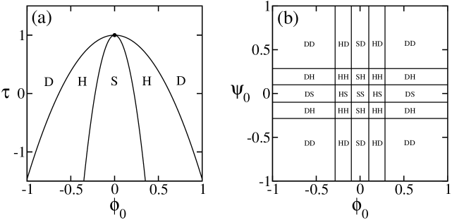
Figure 2: (a) Mean-field phase diagram of a single monolayer with a modulated structure in the vicinity of the critical temperature, computed using a model as in Eqs. (5)-(7). $\phi_{0}$ is the average composition and $\tau$ is the reduced temperature. The three phases are: striped (S), hexagonal (H), and disordered (D). These phases are separated by first-order transition lines, while for clarity we omit showing coexistence regions. The filled circle located at $(\phi_{0},\tau)=(0,1)$ indicates the critical point. Note the shift of the critical temperature from zero to unity when the modulated phases are considered. (b) Mean-field phase diagram of decoupled ($\Lambda=0$) modulated monolayers at $\tau=0.8$. $\phi_{0}$ and $\psi_{0}$ are the average compositions in the two leaflets. The notations of the different phases are described in the text (see Sec. III.1). All the phases are separated by first-order transition lines.

The phase behavior for uncoupled case, $\Lambda=0$, can be obtained from the analysis of $F_{\rm u}[\phi]$ LA and is only briefly reviewed here (see also Fig. 2). For a 2D system, the mean-field phase diagram can be constructed by comparing the free energies of striped (S) and hexagonal (H) phases. In terms of the $\phi$ order parameter, the stripe phase is described by

$$\phi_{\rm S}(\mathbf{r})=\phi_{0}+2\phi_{q}\cos(q^{\ast}x),$$ (2)

where $\phi_{0}=\langle\phi\rangle$ is the spatially averaged composition (imposed by the chemical potential $\mu_{\phi}$), and $\phi_{q}$ is the amplitude of the $q^{\ast}$-mode in the $x$-direction. Similarly, the composition of the hexagonal phase is given by a superposition of three 2D modes of equal magnitude, $|\mathbf{q}_{i}|=q^{\ast}$

$$\phi_{\rm H}(\mathbf{r})=\phi_{0}+\frac{2\phi_{q}}{\sqrt{3}}\sum_{i=1}^{3}\,\cos(\mathbf{q}_{i}\cdot\mathbf{r}),$$ (3)

where

$$\mathbf{q}_{1} = q^{\ast}\hat{x},$$

$$\mathbf{q}_{2} = \frac{q^{\ast}}{2}\left(-\hat{x}+\sqrt{3}\hat{y}\right),$$

$$\mathbf{q}_{3} = \frac{q^{\ast}}{2}\left(-\hat{x}-\sqrt{3}\hat{y}\right),$$ (4)

and $\sum_{i=1}^{3}\mathbf{q}_{i}=0$. In the above, only the most unstable wavenumber $q^{\ast}$ is used within the single-mode approximation. This can be justified for the weak segregation region close to the critical point GD .

Averaging over one spatial period, we obtain the free energy densities of the striped, hexagonal, and disordered phases, respectively

$$f_{\rm S}(\phi_{0},\phi_{q})=\frac{\tau}{2}\phi_{0}^{2}+\frac{1}{4}\phi_{0}^{4}+(\tau-1+3\phi_{0}^{2})\phi_{q}^{2}+\frac{3}{2}\phi_{q}^{4},$$ (5)

$$f_{\rm H}(\phi_{0},\phi_{q})=\frac{\tau}{2}\phi_{0}^{2}+\frac{1}{4}\phi_{0}^{4}+(\tau-1+3\phi_{0}^{2})\phi_{q}^{2}+\frac{4}{\sqrt{3}}\phi_{0}\phi_{q}^{3}+\frac{5}{2}\phi_{q}^{4},$$ (6)

$$f_{\rm D}(\phi_{0})=\frac{\tau}{2}\phi_{0}^{2}+\frac{1}{4}\phi_{0}^{4},$$ (7)

In Fig. 2(a), we reproduce the original phase diagram of Ref. ABJ ; LA . The striped, hexagonal, and disordered phases are separated by first-order phase-transition lines. Regions of two-phase coexistence do exist but are omitted from the figure for clarity sake YK . Thus, the transition lines indicate the locus of points at which the free energies of two different phases cross each other, and are not the proper phase boundaries (binodals). The critical point (filled circle) is located at $(\phi_{0},\tau)=(0,1)$.

III Two Coupled Leaflets with the Same $q^{\ast}$

Having introduced the free energy and explained the phase behavior of the uncoupled case, we shall now explore the equilibrium and non-equilibrium properties of two coupled modulated monolayers, $\Lambda\neq 0$.

III.1 Free Energy Densities

First we consider the case when $D=C=1$ so that the preferred wavenumbers are the same for both monolayers, $q_{\phi}^{\ast}=q_{\psi}^{\ast}=q^{\ast}=1/\sqrt{2}$. The mean-field phase diagram is calculated within the single-mode approximation. Various combinations of 2D modulated structures appearing in the two monolayers are possible. The first example is the striped-striped (SS) phase, in which both monolayers exhibit the striped phase. This can be expressed as

$$\phi_{\rm S}(\mathbf{r})=\phi_{0}+2\phi_{q}\cos(q^{\ast}x),$$ (8)

$$\psi_{\rm S}(\mathbf{r})=\psi_{0}+2\psi_{q}\cos(q^{\ast}x),$$ (9)

where $\phi_{0}=\langle\phi\rangle$ and $\psi_{0}=\langle\psi\rangle$ are the average compositions, $\phi_{q}$ and $\psi_{q}$ are the respective amplitudes. These composition profiles are substituted into the free energy of Eq. (1). Averaging over one spatial period, we obtain the free energy density of the SS phase:

$$f_{\rm SS}=f_{\rm S}(\phi_{0},\phi_{q})+f_{\rm S}(\psi_{0},\psi_{q})-\Lambda(\phi_{0}\psi_{0}+2\phi_{q}\psi_{q}),$$ (10)

where $f_{\rm S}$ is defined in Eq. (5). We then minimize $f_{\rm SS}$ with respect to both $\phi_{q}$ and $\psi_{q}$ for given $\phi_{0}$, $\psi_{0}$, $\tau$ and $\Lambda$. When either $\phi_{q}$ or $\psi_{q}$ vanishes, the corresponding monolayer is in its disordered phase and the mixed bilayer state will be called the striped-disordered (SD) or the disordered-striped (DS) phase. Note that we use the convention that the first index is of the $\phi$–leaflet and the second of the $\psi$–one. When both $\phi_{q}$ and $\psi_{q}$ are zero, the free energy density of the disordered-disordered (DD) phase is given by

$$f_{\rm DD}=f_{\rm D}(\phi_{0})+f_{\rm D}(\psi_{0})-\Lambda\phi_{0}\psi_{0},$$ (11)

where $f_{\rm D}$ is defined in Eq. (7). This free energy $f_{\rm DD}$ was analyzed in Ref. PS in order to investigate the macro–phase separation of a bilayer membrane with coupled monolayers. It was shown that the bilayer can exist in four different phases, and can also exhibit a three-phase coexistence.

Similar to the stripe case, the order parameters of the hexagonal-hexagonal (HH) phase can be represented as

$$\phi_{\rm H}(\mathbf{r})=\phi_{0}+\frac{2\phi_{q}}{\sqrt{3}}\sum_{i=1}^{3}\,\cos(\mathbf{q}_{i}\cdot\mathbf{r}),$$ (12)

$$\psi_{\rm H}(\mathbf{r})=\psi_{0}+\frac{2\psi_{q}}{\sqrt{3}}\sum_{i=1}^{3}\,\cos(\mathbf{q}_{i}\cdot\mathbf{r}).$$ (13)

Where the basis of the three $\mathbf{q}_{i}$ was defined in Eq. (4). By repeating the same procedure as for the SS phase, the free energy density of the HH phase is obtained as

$$f_{\rm HH}=f_{\rm H}(\phi_{0},\phi_{q})+f_{\rm H}(\psi_{0},\psi_{q})-\Lambda(\phi_{0}\psi_{0}+2\phi_{q}\psi_{q}),$$ (14)

where $f_{\rm H}$ is defined in Eq. (6). When either $\phi_{q}$ or $\psi_{q}$ vanishes, one of the monolayers is in the disordered phase and the bilayer will be called the hexagonal-disordered (HD) phase or the disordered-hexagonal (DH) phase.

When the normal hexagonal phase in one leaflet is coupled to the inverted hexagonal phase in the other leaflet, it is energetically favorable to have a particular phase shift of $2\pi/3$ between the two hexagonal structures. The order parameters which represent such a different type of hexagonal-hexagonal (HH^∗) phase can be written as

$$\phi_{\rm H}(\mathbf{r})=\phi_{0}+\frac{2\phi_{q}}{\sqrt{3}}\sum_{i=1}^{3}\,\cos(\mathbf{q}_{i}\cdot\mathbf{r}),$$ (15)

$$\psi_{\rm H^{\ast}}(\mathbf{r})=\psi_{0}+\frac{2\psi_{q}}{\sqrt{3}}\sum_{i=1}^{3}\,\cos(\mathbf{q}_{i}\cdot\mathbf{r}+\frac{2\pi}{3}).$$ (16)

The free energy density of the HH^∗ phase is then obtained as

$$f_{\rm HH^{\ast}}=f_{\rm H}(\phi_{0},\phi_{q})+f_{\rm H}(\psi_{0},\psi_{q})-\Lambda(\phi_{0}\psi_{0}-\phi_{q}\psi_{q}).$$ (17)

Another combination which should be considered in the present model is the asymmetric case where one monolayer exhibits the striped phase and the other the hexagonal phase. This striped-hexagonal (SH) phase is expressed as

$$\phi_{\rm S}(\mathbf{r})=\phi_{0}+2\phi_{q}\cos(q^{\ast}x),$$ (18)

$$\psi_{\rm H}(\mathbf{r})=\psi_{0}+\frac{2\psi_{q}}{\sqrt{3}}\sum_{i=1}^{3}\,\cos(\mathbf{q}_{i}\cdot\mathbf{r}).$$ (19)

The free energy density of this SH phase is calculated to be

$$f_{\rm SH}=f_{\rm S}(\phi_{0},\phi_{q})+f_{\rm H}(\psi_{0},\psi_{q})-\Lambda\left(\phi_{0}\psi_{0}+\frac{2}{\sqrt{3}}\phi_{q}\psi_{q}\right).$$ (20)

The phase in which $\phi_{\rm S}$ and $\psi_{\rm H}$ in Eqs. (18) and (19) are interchanged with $\phi_{\rm H}$ and $\psi_{\rm S}$ is called the hexagonal-striped (HS) phase, and its free energy is obtained from the SH phase by noting the $\phi\leftrightarrow\psi$ symmetry. In addition to these phases, we have also taken into account the square-square (QQ) phase expressed by

$$\phi_{\rm Q}(\mathbf{r})=\phi_{0}+\frac{2\phi_{q}}{\sqrt{2}}\left[\cos(q^{\ast}x)+\cos(q^{\ast}y)\right],$$ (21)

$$\psi_{\rm Q}(\mathbf{r})=\psi_{0}+\frac{2\psi_{q}}{\sqrt{2}}\left[\cos(q^{\ast}x)+\cos(q^{\ast}y)\right].$$ (22)

Then its free energy density is given by

$$f_{\rm QQ}=f_{\rm Q}(\phi_{0},\phi_{q})+f_{\rm Q}(\psi_{0},\psi_{q})-\Lambda\left(\phi_{0}\psi_{0}+2\phi_{q}\psi_{q}\right),$$ (23)

where

$$f_{\rm Q}(\phi_{0},\phi_{q})=\frac{\tau}{2}\phi_{0}^{2}+\frac{1}{4}\phi_{0}^{4}+(\tau-1+3\phi_{0}^{2})\phi_{q}^{2}+\frac{9}{4}\phi_{q}^{4}.$$ (24)

However, we will show below that this QQ phase cannot be more stable than the other phases.

III.2 Bilayer Phase Diagrams

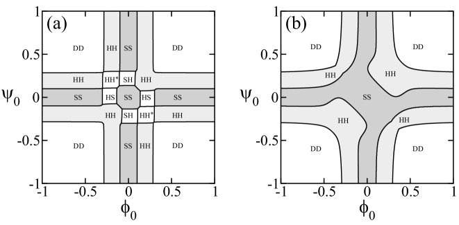
Figure 3: Mean-field phase diagram of coupled modulated bilayers for $\tau=0.8$. $\phi_{0}$ and $\psi_{0}$ are the average compositions in the two leaflets. The coupling parameter is chosen to be (a) $\Lambda=0.02$ and (b) $\Lambda=0.2$. The notations of the different phases are described in the text (see Sec. III.1). All the phases are separated by first-order transition lines. The phase diagram is symmetric with respect to the two principal diagonals $\phi_{0}=\psi_{0}$ and $\phi_{0}=-\psi_{0}$, as described in the text.

Minimizing Eqs. (10), (14), (17), (20) and (23) with respect to both $\phi_{q}$ and $\psi_{q}$, we obtain the phase diagram for the coupled bilayer. As a reference, we first show in Fig. 2(b) the phase diagram in the decoupled case ($\Lambda=0$) for $\tau=0.8$. This can easily be obtained from Fig. 2(a) by combining its two cross-sections (one for $\phi_{0}$ and one for $\psi_{0}$) at $\tau=0.8$. Figure 3 gives the phase diagram for a coupled bilayer when (a) $\Lambda=0.02$ and (b) $\Lambda=0.2$, while the temperature is fixed to $\tau=0.8$ as before. On the $(\phi_{0},\psi_{0})$-plane, we have identified the phase which has the lowest energy, whereas possible phase coexistence regions between different phases have been ignored. All the boundary lines indicate first-order transitions. Since the free energy Eq. (1) is invariant under the exchange of $\phi\leftrightarrow\psi$, the phase diagrams are symmetric about the diagonal line $\phi_{0}=\psi_{0}$ as the upper and lower leaflets have been chosen arbitrarily. These phase diagrams are also symmetric under the rotation of 180 degrees around the origin because Eq. (1) is invariant (except the linear terms) under the simultaneous transformations of $\phi\rightarrow-\phi$ and $\psi\rightarrow-\psi$. This is reasonable as the labels of “A” or “B” for the two lipids have been assigned arbitrarily. As a consequence, the phase diagrams are also symmetric about the diagonal line $\phi_{0}=-\psi_{0}$. The symmetries with respect to both $\phi_{0}=0$ and $\psi_{0}=0$ in Fig. 2(b) for $\Lambda=0$ are now broken because of the coupling between the two leaflets.

When the coupling parameter is small ($\Lambda=0.02$), the global topology of the phase diagram resembles that of the uncoupled case presented in Fig. 2(b). Close to the origin, $\phi_{0}=\psi_{0}=0$, there is a region of SS phase surrounded by eight other phases: two SH, two HS, two HH, and two HH^∗ phases. The HH phase appearing in the region of $\phi_{0}<0$ and $\psi_{0}<0$ is the combination of the two inverted hexagonal structures on each monolayer. One sees that the HH^∗ phase appears in the regions of $\phi_{0}\psi_{0}<0$, where the hexagonal and the inverted hexagonal structures are coupled to each other.

A remarkable feature of this phase diagram is the existence of the SS and HH phases in the regions where either $|\phi_{0}|$ or $|\psi_{0}|$ are large. These outer SS and HH phases extend up to the maximum or the minimum values of the compositions. These regions of the SS and HH phases with $\Lambda>0$ roughly correspond to those of the SD (DS) and HD (DH) phases, respectively, in Fig. 2(b) with $\Lambda=0$. Hence the modulated structure in one of the monolayers induces the same modulated phase in the other monolayer due to the coupling term. Notice that the SD (DS) phase and HD (DH) phase do not exist in Fig. 3(a). We further remark that the extent of the four DD phase regions is almost unaffected by the coupling. Even when the temperature is lowered by decreasing $\tau$, only the phases located close to the origin ($\phi_{0}=\psi_{0}=0$) would expand, and the global topology does not change substantially.

For a larger value of the coupling parameter ($\Lambda=0.2$), the five regions of the SS phase merge together forming one single continuous SS region. The four HH regions and still distinct and separate the SS region from four DD phase regions. Note that in Fig. 3(b), all phases have a symmetric combination of phase modulation such as SS or HH. The asymmetric combination such as the SH phase does not appear, because the large coupling parameter strongly prefers symmetric phases of equal modulations in the two monolayers, although the $\phi_{q}$ and $\psi_{q}$ amplitudes of the two modulated monolayers are not the same in the stripe SS phase (or the hexagonal HH phase). As the value of $\Lambda$ is increased from $0.02$ to $0.2$, first the SH phase disappears, followed by the disappearance of the HH^∗ phase. When the value of $\Lambda$ is further increased, the regions of the SS and HH phases expand on the expense of the DD phase regions. This means that the coupling between the monolayers causes more structural order in the bilayer. Finally we remark that the QQ phase was never found to be more stable than any of the other phases considered above.

Although we have so far assumed that $\Lambda$ is positive, the phase diagrams for $\Lambda<0$ can be easily obtained from those for $\Lambda>0$ by rotating them by 90 degrees around the origin. This is because the free energy Eq. (1) is invariant under the simultaneous transformations of either $\phi\rightarrow-\phi$ and $\Lambda\rightarrow-\Lambda$, or $\psi\rightarrow-\psi$ and $\Lambda\rightarrow-\Lambda$.

III.3 Modulated Bilayer Dynamics

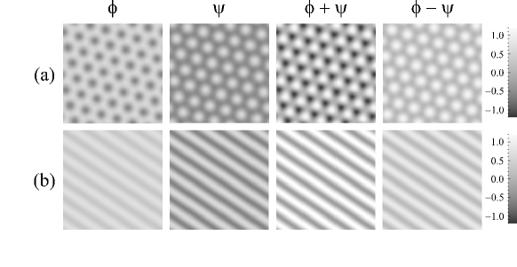
Figure 4: Equilibrium patterns of coupled modulated monolayers with $\tau=0.8$. In addition setting $D=C=1$ implies the same $q^{\ast}$ in both monolayers. The patterns of $\phi$, $\psi$, $\phi+\psi$, and $\phi-\psi$ at $t=5,000$ are presented. The other parameters are chosen to be (a) $\phi_{0}=0.2$, $\psi_{0}=-0.2$, $\Lambda=0.02$, and (b) $\phi_{0}=0.5$, $\psi_{0}=0$, $\Lambda=0.2$.

In order to check the validity of the obtained phase diagram and to investigate the dynamics of coupled modulated bilayers, we consider now the time evolution of the coupled equations for $\phi$ and $\psi$:

$$\frac{\partial\phi}{\partial t}=L_{\phi}\nabla^{2}\frac{\delta F}{\delta\phi},~{}~{}~{}~{}~{}~{}\frac{\partial\psi}{\partial t}=L_{\psi}\nabla^{2}\frac{\delta F}{\delta\psi}.$$ (25)

Here we have assumed that both $\phi$ and $\psi$ are conserved order parameters in each of the monolayer (model B in the Hohenberg-Halperin classification HH ). For simplicity, the kinetic coefficients $L_{\phi}$ and $L_{\psi}$ are taken to be unity, and both the hydrodynamic effect and thermal fluctuations are neglected. We solve the above equations numerically in 2D using the periodic boundary condition. Each simulation starts from a disordered state with a small random noise around the average compositions $\phi_{0}$ and $\psi_{0}$. In Fig. 4, we show typical equilibrium patterns of $\phi$, $\psi$, $\phi+\psi$ and $\phi-\psi$ for two choices of parameters. The $\phi+\psi$ pattern is presented here because this quantity can be directly observed in the experiment on Montal-Mueller bilayers using fluorescence microscopy CK . The quantity $\phi-\psi$ measures the concentration contrast between the $\phi$ and $\psi$ leaflets. Time is measured in discrete time steps, and $t=5,000$ corresponds to a well equilibrated system. In all the simulations below, the temperature is fixed to be $\tau=0.8$ corresponding to the weak segregation regime. Notice that all the patterns in Fig. 4 are presented with the same gray scale.

Figure 4(a) illustrates the coupling between a hexagonal phase with $\phi_{0}=0.2$ and an inverted hexagonal phase with $\psi_{0}=-0.2$ in the weak coupling regime ($\Lambda=0.02$). Being consistent with the phase diagram of Fig. 3(a), this parameter choice yields the HH^∗ phase as seen from the pattern of $\phi+\psi$ where the two hexagonal structures are superimposed. We note that the difference in the order parameter $\phi-\psi$ also exhibits a hexagonal structure.

Figure 4(b) shows the equilibrium patterns for $\phi_{0}=0.5$ and $\psi_{0}=0$ in the strong coupling regime ($\Lambda=0.2$). If there were no coupling, the $\phi$-monolayer would not exhibit any modulation (as it is in its own disordered phase), whereas the $\psi$-monolayer is in the striped phase. We clearly see that, due to the coupling effect, the stripe structure is induced in the pattern of $\phi$. This corresponds to the SS phase shown in Fig. 3(b). The periodicities of the two striped structures are the same, although their amplitudes differ. Notice that the modulation phase of $\phi+\psi$ is shifted by $\pi$ relatively to that of $\phi-\psi$. Since the patterns in Fig. 4 would correspond to the equilibrium configurations, they can be compared with the phase diagrams in Fig. 3. We conclude that these simulation results indeed reproduce the predicted equilibrium modulated structures.

IV Coupled monolayers with two different $q^{\ast}$

We consider next the more general case in which the preferred wavelengths of modulation in the two uncoupled leaflets are different, $q^{\ast}_{\phi}\neq q^{\ast}_{\psi}$. The free energy densities cannot be obtained analytically as was done in Sec. III.1, because there is not a single periodicity on which one can average $\phi(\mathbf{r})$ and $\psi(\mathbf{r})$. Due to such a difficulty in the analytical treatment, we present below the results of numerical simulations, relying on Eq. (25) for the time evolution of the two coupled order parameters.

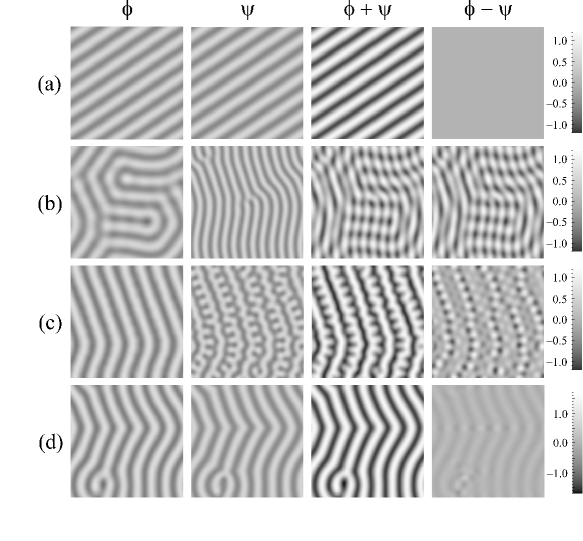
Figure 5: Patterns of coupled modulated monolayers with $\tau=0.8$. The patterns of $\phi$, $\psi$, $\phi+\psi$, and $\phi-\psi$ are presented for simulation time, $t=5,000$, and the average compositions are set to be $\phi_{0}=\psi_{0}=0$. The other parameters are chosen to be (a) $D=C=1$, $\Lambda=0.02$, (b) $D=0.1296$, $C=0.36$, $\Lambda=0.02$, (c) $D=0.1296$, $C=0.36$, $\Lambda=0.2$, and (d) $D=0.1296$, $C=0.36$, $\Lambda=0.4$. In all cases but (a), $D\neq C$ and the two periodicities are nonequal, $q^{\ast}_{\phi}\neq q^{\ast}_{\psi}$.

Figure 6: Time evolutions of $\Delta$ defined by Eq. (26). The solid, dashed, dotted, and dashed-dotted lines correspond to the parameters of Fig. 5(a), (b), (c) and (d), respectively.

In Fig. 5, we show the patterns for $\tau=0.8$ and $\phi_{0}=\psi_{0}=0$, when both monolayers exhibit the striped phase without the coupling. As a reference, we show in Fig. 5(a) the case when $D=C=1$ and $\Lambda=0.02$ corresponding to the SS phase in Fig. 3(a). The patterns of $\phi$ and $\psi$ match each other as the composition difference $\phi-\psi$ vanishes throughout the system. In Fig. 5(b), the parameters are chosen to be $D=0.1296$, $C=0.36$ and $\Lambda=0.02$. The preferred wavenumbers of the two monolayers are different: $q_{\psi}^{\ast}=1.67q_{\phi}^{\ast}$ for uncoupled leaflets. The above set of parameters, especially $D$ and $C$, are chosen in such a way that the amplitudes of the two stripes are nearly equal. As long as the coupling parameter is small, the two stripes of different periodicities are formed rather independently. The superposition of the two striped structures produces an interference pattern resulting in a new modulation as seen from the pattern of $\phi+\psi$. The striped modulations of $\phi$ and $\psi$ are almost parallel or perpendicular to each other.

When $\Lambda$ is made larger, up to $\Lambda=0.2$ as in Fig. 5(c), the $\psi$ field exhibits a complex pattern in which two different length scales coexist (reflecting $q_{\phi}^{\ast}$ and $q_{\psi}^{\ast}$), whereas the pattern of $\phi$ is characterized by a single mode (reflecting $q_{\phi}^{\ast}$). The patters of $\phi$ and $\psi$ almost match each other when $\Lambda=0.4$ as seen in Fig. 5(d). In this case, the modulation with a longer wavelength ($q_{\phi}^{\ast}$) dominates both monolayers. Figure 5(b), (c), (d) provide a typical sequence of morphological changes, i.e., interference pattern $\rightarrow$ two-mode pattern $\rightarrow$ single-mode pattern, as the coupling constant $\Lambda$ is increased.

To further analyze the temporal correlations of the two order parameters, $\phi$ and $\psi$, we have plotted in Fig. 6 the time evolution of the quantity

$$\Delta(t)=\frac{1}{L^{2}}\int{\rm d}\mathbf{r}\,[\phi(\mathbf{r},t)-\psi(\mathbf{r},t)]^{2},$$ (26)

where $L=128$ is the linear system size in the simulations. The solid, dashed, dotted, and dashed-dotted lines correspond to the time evolutions of $\Delta(t)$ in Fig. 5(a), (b), (c), and (d) respectively. The solid line (a) first increases and then approaches to zero since the patterns of the two stripes coincide in the late stage. The dashed line (b) increases in two separate stages. At first because the growth rate of the modulation having smaller wavelength (corresponding to $\psi$) is faster than that having larger periodicity (corresponding to $\phi$) as is also revealed from the linear stability analysis of Eq. (25) which will be published elsewhere. At late temporal stages, the value of $\Delta$ remains large for small coupling parameter ($\Lambda=0.02$). When the coupling becomes even stronger ($\Lambda=0.2$) as for the dotted line (c), the value of $\Delta$ is suppressed compared to the dashed line (b), because $\phi$ and $\psi$ tend to have more overlap for larger $\Lambda$. The same applies for the dashed-dotted line (d) with $\Lambda=0.4$ as compared to the dotted line (c).

V Discussion

We propose a minimal model describing the coupling phenomena between two modulated bilayers. Considering 2D case, we obtain the mean-field phase diagram when the two coupled and spatially modulated monolayers have the same preferred periodicity. Various combinations of modulated phases can exist such as the SS, HH, HH^∗ and SH (HS) phases as described in Sec. III. We have seen that modulations in one of the monolayers induces a similar modulations in the other. The region of the induced modulated phase expands as the coupling parameter becomes larger.

When the two monolayers have different inherent wavelengths in the decoupled case, we have conducted numerical simulations to investigate the morphologies and dynamics of the coupled system. We obtain several complex patterns arising from the frustration induced by the two incommensurate structures. As the coupling constant $\Lambda$ is made larger, the two different modes start to interfere with each other and eventually coincide. The time evolution of the striped structures can take place in two steps reflecting the different growth rate of the two modulations.

It is instructive to rewrite the free energy Eq. (1) in terms of the sum and the difference of $\phi$ and $\psi$ with $\eta_{\pm}=\phi\pm\psi$. When $D=C=1$, we obtain

$$F[\eta_{+},\eta_{-}] =\int{\rm d}\mathbf{r}\biggl{[}(\nabla^{2}\eta_{+})^{2}-(\nabla\eta_{+})^{2}+\frac{1}{4}(\tau-\Lambda)\eta_{+}^{2}+\frac{1}{32}\eta_{+}^{4}-\mu_{+}\eta_{+}$$

$$+(\nabla^{2}\eta_{-})^{2}-(\nabla\eta_{-})^{2}+\frac{1}{4}(\tau+\Lambda)\eta_{-}^{2}+\frac{1}{32}\eta_{-}^{4}-\mu_{-}\eta_{-}+\frac{3}{16}\eta_{+}^{2}\eta_{-}^{2}\biggr{]},$$ (27)

where $\mu_{\pm}=(\mu_{\phi}\pm\mu_{\psi})/2$. Hence the coupling term between $\eta_{+}$ and $\eta_{-}$ in the free energy takes the form of an $\eta_{+}^{2}\eta_{-}^{2}$ term with a numerical positive coefficient. The original coupling parameter $\Lambda$ enters in the coefficients of $\eta_{+}^{2}$ and $\eta_{-}^{2}$ terms (but not in the $\eta_{+}^{2}\eta_{-}^{2}$ coupling term). It shifts the respective transition temperatures of $\eta_{+}$ and $\eta_{-}$ in opposite directions. When the gradient terms are absent and $\mu_{-}=0$, a similar model was considered by MacKintosh and Safran who studied transitions between lamellar and vesicle phases in two-component fluid bilayers MS .

The proposed free energy Eq. (1) has some analogies to the previous model for the rippled phase in lipid bilayers KK . It was argued that the coupling between the membrane curvature and the asymmetry in the area per molecule between the two monolayers would induce a structural modulation of a bilayer. By considering a similar mechanism, Kumar et al. KGL investigated various modulated phases in two-component bilayer membranes. They claimed that the phase behavior of two-component bilayers resembles that of three-component monolayer. This is because the three different local combinations of upper/lower composition in bilayers (A/B, B/A, and A/A for excess of A), would correspond to three different types of molecules for the monolayer. One of the new aspects in our model is that the preferred wavelengths of the two monolayers can, in general, be different from one another leading to a frustrated bilayer state.

We also point out that there are some similarities between coupled modulated structures and the problem of atoms adsorbed on a periodic solid substrate. The latter topic has been extensively studied within the Frenkel-Kontorova (FK) model which provides a simple description of the commensurate-incommensurate transition CL . Our model and the FK model are analogous in the sense that there are two natural length scales whose ratio changes as a function of other model parameters. In the FK model, however, these length scales are quenched, whereas in our model they are annealed.

Another related experimental system can be seen for surface-induced ordering in thin film of diblock copolymers TA . When the surface is periodically patterned, a tilt of the lamellae is induced in order to match the surface periodicity. The situation becomes more complex if a copolymer melt is confined between two surfaces. An interesting case arises when the spacing between the two surfaces is incommensurate with the lamellar periodicity TA .

For systems out of equilibrium, spatial resonances and superposition patterns combining stripes and/or hexagons were investigated in a reaction-diffusion model with interacting Turing modes of different wavelengths YDZE . These models were successful in reproducing hexagonal superlattice patterns which are known as “black-eyes”. Although the mechanism of pattern formation is different than in our model, we observe similar superposition patterns as reported in Ref. YDZE , such as hexagons on stripes or hexagons on hexagons (not shown in this paper).

A more detailed study of the present model and several interesting extensions will be published elsewhere. One possible extension is to consider vector order parameters describing, for example, the molecular tilt for coupled bilayers CLM ; SSN . When the two order parameters are vectors, the nature of the transitions between different phases can be different, and even the square phase may exist in thermodynamic equilibrium TLFKH .

- (1) M. Seul and D. Andelman, Science 267, 476 (1995).
- (2) D. Andelman and R. E. Rosensweig, J. Phys. Chem. B 113, 3785 (2009).
- (3) D. Andelman and R. E. Rosensweig, Polymers, Liquids and Colloids in Electric Fields: Interfacial Instabilities, Orientation and Phase Transitions, edited by Y. Tsori and U. Steiner (World Scientific, Singapore, 2009).
- (4) C. L. Dennis, R. P. Borges, L. D. Buda, U. Ebels, J. F. Gregg, M. Hehn, E. Jouguelet, K. Ounadjela, I. Petej, I. L. Prejbeanu, and M. J. Thornton, J. Phys.: Condens. Matter 14, R1175 (2002).
- (5) T. Garel and S. Doniach, Phys. Rev. B 26, 325 (1982).
- (6) R. E. Rosensweig, Ferrohydrodynamics (Cambridge University, New York, 1985).
- (7) D. Andelman, F. Brochard, and J.-F. Joanny, J. Chem. Phys. 86, 3673 (1987).
- (8) E. Sackmann, Structure and Dynamics of Membranes: From Cells to Vesicles, edited by R. Lipowsky and E. Sackmann (Elsevier, Amsterdam, 1995).
- (9) I. W. Hamley, The Physics of Block Copolymers (Oxford University, Oxford, 1998).
- (10) G. H. Fredrickson, The Equilibrium Theory of Inhomogeneous Polymers (Oxford University, Oxford, 2005).
- (11) S. Leibler and D. Andelman, J. Phys. (France) 48, 2013 (1987).
- (12) M. D. Collins and S. L. Keller, Proc. Natl. Acad. Sci. USA 105, 124 (2008).
- (13) M. Montal and P. Mueller, Proc. Natl. Acad. Sci. USA 69, 3561 (1972).
- (14) A. J. Wagner, S. Loew, and S. May, Biophys. J. 93, 4268 (2007).
- (15) G. G. Putzel and M. Schick, Biophys. J. 94, 869 (2008).
- (16) S. L. Keller, W. H. Pitcher, W. H. Huestis, and H. M. McConnell, Phys. Rev. Lett. 81, 5019 (1998).
- (17) S. L. Keller and H. M. McConnell, Phys. Rev. Lett. 82, 1602 (1999).
- (18) L. Leibler, Macromolecules 13, 1602 (1980).
- (19) G. Gompper and M. Schick, Phys. Rev. Lett. 65, 1116 (1990).
- (20) R. R. Netz, D. Andelman, and M. Schick, Phys. Rev. Lett. 79, 1058 (1997).
- (21) S. Villain-Guillot and D. Andelman, Eur. Phys. J. B 4, 95 (1998).
- (22) S. Villain-Guillot, R. R. Netz, D. Andelman, and M. Schick, Physica A 249, 285 (1998).
- (23) S. May, Soft Matter ??, ???? (2009).
- (24) K. Yamada and S. Komura, J. Phys.: Condens. Matter 20, 155107 (2008).
- (25) P. C. Hohenberg and B. I. Halperin, Rev. Mod. Phys. 49, 435 (1977).
- (26) F. C. MacKintosh and S. A. Safran, Phys. Rev. E 47, 1180 (1993).
- (27) H. Kodama and S. Komura, J. Phys. II 3, 1305 (1993).
- (28) P. B. S. Kumar, G. Gompper, and R. Lipowsky, Phys. Rev. E 60, 4610 (1999).
- (29) P. M. Chaikin and T. C. Lubensky, Principles of Condensed Matter Physics (Cambridge University, Cambridge, 1995).
- (30) Y. Tsori and D. Andelman, J. Chem. Phys. 115, 1970 (2001).
- (31) L. Yang, M. Dolnik, A. M. Zhabotinsky, and I. R. Epstein Phys. Rev. Lett. 88, 208303 (2002).
- (32) C.-M. Chen, T. C. Lubensky, and F. C. MacKintosh, Phys. Rev. E 51, 504 (1995).
- (33) U. Seifert, J. Shillcock, and P. Nelson, Phys. Rev. Lett. 77, 5237 (1996).
- (34) C. Tang, E. M. Lennon, G. H. Fredrickson, E. J. Kramer, and C. J. Hawker, Science 322, 429 (2008).