A Refined Tully-Fisher Relationship and a New Scaling Law for Galaxy Discs.

Abstract

We show how the hypothesis that galaxy discs conform to self-similar dynamics leads to the identification of an annular region of the optical disc which is such that, corresponding to the Tully-Fisher scaling law defined on the exterior annular boundary, there is a similar scaling law defined on the interior annular boundary. This result is confirmed at the level of statistical certainty over several large ORC samples. Furthermore, the same analysis provides insight into the uncertainties associated with the “best” way of defining $V_{max}$, the rotation velocity used for the Tully-Fisher scaling law and $R_{max}$, the galaxy radius at which $V_{max}$ is measured. Finally, as a direct consequence, we are led to a refined Tully-Fisher law which is largely insensitive to the means by which a galaxy’s rotation velocity is defined.

1 Introduction

1.1 General comments

One of the many problems which hinders our understanding of the underlying primary processes driving spiral galaxies is the fact that such galaxies are frequently observed to be “afflicted” by one of the following:

1. ongoing interactions with external objects;

2. manifest signatures of such interactions in the near past;

3. internal inhomogeities generating local perturbations;

4. presence of bars;

5. unusually active central regions,

and so on. The net effect of these various phenomena is to considerably complexify the task of identifying the irreducible physics and phenomenology which define the essential nature of the spiral galaxy.

1.2 Structure suggesting self-similar dynamics in annular discs

Regardless of the foregoing problems, there still exist various (statistically) strong signatures which appear to be fundamental; these are:

1. the existence of the Tully-Fisher scaling relationship ($M\approx a_{0}+b_{0}\log V_{max}$);

2. the long-standing recognition (Danver 1942, Kennicutt 1981) that the spirality of the spiral arms in disc galaxies can be usefully classified in terms of the logarithmic spiral, $R=R_{0}\exp(b\theta)$, for radial displacement $R$ and angular displacement $\theta$.

The second of these signatures, in particular, is consistent with the hypothesis that the dynamics in spiral discs conform to laws of self-similarity. That is, in the annular sub-regions where spirality is manifest,

$$\frac{V_{rot}}{V_{rad}}=\frac{\dot{V}_{rot}}{\dot{V}_{rad}}=...=constant,$$

from which, immediately,

$$V_{rot}=Af(R),\,\,\,V_{rad}=Bf(R)$$ (1)

for some undetermined function $f(R)$ and constants $(A,B)$. There are some obvious comments to be made:

1. Since spirality is a property restricted to an annular region of galaxy discs, and since the (logarithmic) spirality property is implied by (1), then this latter hypothesized velocity field must be considered confined to some annular region. The precise quantitative definition of this annular region is given in §3.1;

2. There is a large amount of galaxy rotation data available which makes a statistical study of $V_{rot}$ perfectly feasible so that, in principle, it is possible to hypothesize and test specific proposals for $f(R)$;

3. Until recently, it was thought that there were essentially no systematic radial flows in galaxy discs - presumably because of the mass-flow implications - but it is becoming increasingly recognized that radial flows are a common feature of galaxy discs so that, in principle at least, we can conceive the possibility $V_{rad}\propto V_{rot}$ for the typical galaxy disc. However, the very small amount of radial flow data presently available renders any large scale statistical study of radial flows impossible, for some years at least.

1.3 An hypothesis for $f(R)$ and the manner of its testing

The topic of how best to express rotation curves in some generic functional form has received much attention over the years; but all of these efforts have been focussed on the whole rotation curve. By contrast, here we are concerned only with the rotation curve in a limited annular region (to be precisely defined in §3.1) of the optical domain where self-similar behaviour appears to be manifested - that is, we are not concerned with rotation curve behaviour in the interior regions, and nor are we concerned with the behaviour where they tend to become (approximately) flat. The most simple possibility that has any chance of accommodating the variation between discs for the two-dimensional velocity field in the optical annulus only is $f(R)\equiv R^{\alpha}$, so that our hypothesis becomes

$$V_{rot}\approx AR^{\alpha},\,\,\,V_{rad}\approx BR^{\alpha},\,\,\,R_{min}\leq R\leq R_{max}$$

where $R_{min}$ and $R_{max}$ defined the boundaries of the annular region to be defined in §3.1. However, as we have already indicated, it is only feasible to consider whether or not $V_{rot}\approx AR^{\alpha}$ at the moment. We assess the validity of the power-law hypothesis in qualitative and quantitative analyses and briefly describe these in the immediately following.

1.3.1 Qualitative assessment

The adoption of the power-law hypothesis $V_{rot}=AR^{\alpha}$ for the annular disc leads directly to the following results:

1. the classical Tully-Fisher scaling relationship,

   $$M_{TF}\approx a_{0}+b_{0}\log V_{max},$$

   defined on the exterior boundary of the annular disc, emerges automatically from the correlation which is found to exist between the power-law parameters $\left(A,\alpha\right)$ and global luminosity properties;

2. the power-law exponent, $\alpha$, which can be estimated independently of distance scales being determined, allows the definition of an enhanced Tully-Fisher relation of the type

   $$M_{TF}=a+(b+\alpha c)\log V_{max}\,,$$

   where $V_{max}$ can be defined in many ways without appreciably affecting the quality of the resulting $M_{TF}$ determinations;

3. corresponding to the Tully-Fisher scaling relationship on the exterior boundary of the annular disc, there is a directly analogous scaling relationship

   $$M_{TF}\approx a_{1}+b_{1}\log V_{min}$$

   defined on the interior boundary of the annular disc. This result is entirely new, and lead to the identification of the dynamically coherent annular disc as an objective reality.

The fact that these quantitative results arise directly from the hypothesis of $V_{rot}=AR^{\alpha}$ for the annular disc provides considerable circumstantial support for the hypothesis.

1.3.2 Quantitative assessment

Generally speaking, when considering power-law fits to data, it is not possible to say anything more than the power-law does/does not provide a good fit. In the present case, for various reasons, we can go much further: we are able to say that, for all practical purposes, the data behaves as if $V_{rot}=AR^{\alpha}$ is the fundamental law and not merely just a good fit.

This is done in the following way: we note that any whole-disc rotation curve can be expressed as

$$\frac{V_{rot}}{V_{0}}=\left(\frac{R}{R_{0}}\right)^{\alpha}+g\left(\frac{R}{R_{0}}\right),$$ (2)

for arbitrary values $\left(R_{0}>0,V_{0}>0,\,\alpha\right)$ and for some suitably chosen function, $g(R/R_{0})$. We are able to show that for each ORC in the large samples considered, values of $\left(R_{0},V_{0},\alpha\right)$ can be chosen (uniquely for each disc) such that

$$\log\left[1+\left(\frac{R_{0}}{R}\right)^{\alpha}g\left(\frac{R}{R_{0}}\right)\right]\approx N(\bar{x},\sigma)\,\,\,{\rm where}\,\,\bar{x}\approx 0,\,\,\sigma<<1,$$

over the annular discs of the galaxies concerned. In other words, $g(R/R_{0})$ itself behaves similarly to a log-normal random variable with a mean close to zero. For example, for the case of the Mathewson, Ford and Bucchorn (1992) sample of 900 ORCs, we find $N(\bar{x},\sigma)\approx N(0.002,\,0.07)$.

The implication of this latter result is that, over large samples, the rotational dynamics on the annular disc (to be given an objective operational definition) are described to high precision in a least-square sense by $V\approx\left[V\right]_{model}\equiv AR^{\alpha}$, where $(A,\alpha)$ are parameters determined by the ORC in the annular disc. Alternatively, we can say that deviations from simple power law behaviour in the annular disc are normally distributed with a mean close to zero.

2 The rotation curve samples

The optical rotation curve samples considered in this analysis are those of:

1. Mathewson, Ford & Bucchorn (1992) which consists of 900 objects hereafter referred to as MFB;

2. Mathewson and Ford (1996) which consists of 1200 objects, hereafter referred to as MF;

3. Courteaux (1997) which consists of 305 objects, hereafter referred to as SC;

4. A composite sample collected from Dale, Giovanelli and Haynes (1997, 1998, 1999) and Dale & Uson (2000) consisting of 497 objects, hereafter referred to as DGHU. This sample was provided by permission of Giovanelli and Haynes.

2.1 The folding of rotation curves

The analysis to be described is predicated upon the ability to fold rotation curves with high precision and, in this, Persic, Salucci & Stel (Persic, M., Salucci, P., & Stel, F. 1996, MNRAS, 281, 27) laid out the basic approach to be adopted.

Traditionally, the ‘quick and dirty‘ approach to folding involves simply identifying the photometric centre of a disc (an unambiguous process) and then subtracting the observed redshift at that point from the whole rotation curve. This approach is perfectly acceptable if one is primarily interested in the bulk-flow of galaxies. But, if ones primary interest is in the internal dynamics of the galaxies themselves (as was Persic et al’s), then it is necessary to recognize that the centre of rotation of a galaxy (its kinematic centre) does not necessarily coincide with its photometric centre. Persic et al found that the best results were obtained if the centre of folding (the kinematic centre) and the systematic recession velocity were treated as two free parameters, to be determined such that the ‘folded arms were maximally matched‘.

The difficulty, of course, is in deciding what is meant by ‘maximally matched‘ - especially given that rotation curves are, more often than not, unevenly sampled in some way; for example, the measurements may not extend equally on either side of the disc, or measurements may be taken at unequal intervals on either side of the disc, etc. Persic et al adopted a labour-intensive, non-automated and qualitative ‘eye-ball‘ approach to the problem, whilst Catinella, Haynes and Giovanelli (AJ, 130, 10371048, 2005) have constructed a method based upon using the two parameters to optimize the fit of Persic et al’s Universal Rotation Curve function to their rotation curves.

The automatic algorithm developed by this author (A&A Supp, 140, 247-260, 1999) is also based upon Persic et al’s two-parameter method and, briefly, operates as follows:

The two parameters are varied such that, in a Fourier decomposition of the whole rotation curve (which is purely asymmetric in the ideal case), a normalized measure of the residual symmetric components is minimized.

Due to various problems, such as asymmetric sampling or how many Fourier modes to use for any given ORC etc, the actual implementation of this simple algorithm is complicated, but the code is available from this author.

Finally, one very important point, identified by Persic et al, is that, given a whole set of velocity measurements over a rotation curve it is necessary to also have quantitative estimates of the absolute accuracy of each individual velocity measurement available - and then to use this information as a means of filtering out only the best individual measurements for the folding process. Broadly speaking, any individual velocity measurement is retained only if its estimated absolute error $\leq 5\%$. For the MFB, MF, SC and DGHU samples, this requirement led to losses of $35\%$, $25\%$, $46\%$ and $46\%$ respectively of all individual velocity measurements. The net effect of these data losses meant that many ORCs were then left with insufficient data points on them to permit a reliable folding. The overall attrition rate of ORCs lost to the overall analysis via this process were $3\%$, $4\%$, $7\%$ and $8\%$ respectively.

3 The annular disc: A dynamically coherent whole

The most significant result of this section is the demonstration that the annular disc is a dynamically coherent and objectively defined component of the total disc. Apart from giving the algorithmic definition of the annular disc, the demonstration consists in showing how the interior boundary of the annular disc is a dynamical transition region between the inner and outer parts of the disc on which a scaling law, directly analogous to the classical Tully-Fisher scaling law, is defined.

3.1 Extraction of the annular disc from the whole disc

The process to be described is based on the hypothesis that $V\approx\left[V\right]_{model}\equiv AR^{\alpha}$ describes rotation velocities in ORCs in certain annular regions which are to be extracted from the whole disc. Before describing the extraction algorithm, there are two important notes to be made:

1. By the ‘whole disc‘ in this context, we mean the complete set of velocity data for the disc with the exception of any filtered-out poor-quality individual measurements (cf last section). The annular disc is extracted from the whole disc using a statistical algorithm based upon the technique of linear regression: following conventional definitions, an observation is reckoned to be unusual if the predictor is unusual, or if the response is unusual. For a $p$-parameter model, a predictor is commonly defined to be unusual if its leverage $>3p/N$, when there are $N$ observations. In the present case, we have a two-parameter model so that $p=2$. Similarly, the response is commonly defined to be unusual if its standardized residual $>2$.

2. The prescription $V\approx AR^{\alpha}$ can only be completely specified for any given ORC when the distance scale has been set. However, the exponent $\alpha$ is independent of the distance scale; consequently, the identification of any annular region over which the approximate power-law may be valid is also independent of the distance scale. For this reason, the extraction algorithm described below assumes that radial displacements are specified in radians, $R_{(radians)}$ say; the corresponding calculated $A$ is denoted as $A^{*}$.

The computation of $(\alpha,\ln A^{*})$, for any given folded and inclination-corrected rotation curve, can now be described using the following algorithm:

1. Assume the model $V\approx\left[V\right]_{model}=A^{*}R_{(radians)}^{\alpha}$ for the rotation velocity in some annular region of the disc, to be determined. But initially, use the whole disc ORC;

2. Form an estimate of the parameter-pair $(\alpha,\ln A^{*})$ by regressing the $\ln V$ data on the $\ln R_{(radians)}$ data for the folded ORC;

3. Determine if the innermost observation only is an unusual observation in the sense defined above;

4. If the innermost observation is unusual, then exclude it from the computation and repeat the process from (2) above on the reduced data-set;

5. If the innermost observation is not unusual, then no further computation is required:

   1. the remaining set of points at this stage are considered to define the extracted annular region. The minimum value of $R$ for any given disc, $R_{min}$ say, defines the radius of the interior boundary of the extracted annulus and $V_{min}$ denotes the rotation velocity on this interior boundary;

   2. the current value of $\alpha$ defines the exponent of the power-law over the extracted annular region;

   3. the value $A^{*}$ has no particular significance since a distance scale has yet to be set.

This algorithm has the result that, on average, $(\alpha,\ln A^{*})$ is computed on the exterior 88% of the data points in each ORC of the MFB sample, the exterior 87% of data points in each ORC of the MF sample, the exterior 91% of data points in each ORC of the DGHU sample and the exterior 91% of the data points in each ORC of the SC sample.

3.2 An old result quantified and refreshed

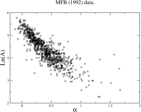
Figure 1:

It has been known for a long time that, in a qualitative sense, the steeper the rise of a rotation curve on its interior portion, then the flatter the rotation curve is in its exterior portion.

Given our hypothesis that $V\approx AR^{\alpha}$ on the annular disc, then it is clear that the parameter $A$ has the numerical value of the approximate rotation velocity at 1$kpc$ (given that $R$ is in units of $kpc$) - as estimated by using the power law to extrapolate (or interpolate) the data to 1$kpc$. It follows that the value of $A$ can also be considered as a proxy measure for the steepness of the initial rise of the rotation curve in which case, given the qualitative statement above, we should expect $A$ and $\alpha$ to be in an inverse relation to each other.

For the sake of demonstrating the reality of this relationship, we use MFB’s Tully-Fisher distances to set the radial distance scale so that $A$ can be computed for each galaxy in sample. Figure 1 then shows the scatter diagram plotting $(\alpha,\ln A)$, computed as in §3.1 for each foldable galaxy in the Mathewson et al (1992) sample. The powerful nature of their inverse relation is clearly apparent.

To summarize, the given analysis quantifies old qualitative knowledge by providing an explicit and well-defined partition of the optical disc into distinct dynamical regions: the interior disc containing the steep initial rise, and the exterior annular disc over which - as we shall demonstrate - the rotational dynamics are described to extremely high fidelity by the $V\approx AR^{\alpha}$.

3.3 Scaling laws and the annular disc

The algorithm described in §3.1 will always produce a result in the form of an extracted annular disc. So, the significant questions are:

1. Does the process described have any basis in physics so that the annular disc can be identified as a physically coherent distinct sub-component of the whole disc ?

2. Or is the data reduction process essentially arbitrary, the product of which has no physical significance whatsoever?

In the following, we show that a scaling law similar to the Tully-Fisher law which applies at the exterior boundary of the annular disc also applies on its interior boundary, $R\equiv R_{min}$ determined in §3.1, and at similar levels of statistical significance. Thus, this interior boundary is a boundary of objective physical significance which scales according to luminosity and which defines, in effect, the transition within the disc between one form of behaviour and another.

3.3.1 The interior Tully-Fisher law

In the following, we establish the existence of a Tully-Fisher-type law on the interior boundary of the annular disc. The results of the individual regressions are given below:

$${\rm MFB:}\,\,\,\,M_{TF} \approx (-14.60\pm 0.15)+(-1.40\pm 0.03)\ln V_{min}\,,$$

$$n=849,\,\,\,t_{grad}=-42,\,\,R_{adj}^{2}=67\%\,;$$

$${\rm MF:}\,\,\,\,M_{TF} \approx (-14.79\pm 0.13)+(-1.36\pm 0.03)\ln V_{min}\,,$$

$$n=1070,\,\,t_{grad}=-45,\,\,R_{adj}^{2}=65\%\,;$$

$${\rm SC:}\,\,\,\,M_{TF} \approx (-14.89\pm 0.26)+(-1.36\pm 0.05)\ln V_{min}\,,$$

$$n=275,\,\,\,\,t_{grad}=-25,\,\,R_{adj}^{2}=69\%\,;$$

$${\rm DGHU:}\,\,\,\,M_{TF} \approx (-11.81\,\pm 0.24)+(-1.95\pm 0.05)\ln V_{min}\,,$$

$$n=487,\,\,\,\,t_{grad}=-38,\,\,R_{adj}^{2}=75\%\,.$$

The quoted $t$-statistic is each case refers to the estimated gradient value and it is quite obvious that, in every case, the dependence of the Tully-Fisher estimated absolute luminosity, $M_{TF}$, upon the rotational velocity on the interior boundary of the annular disc is established at the level of statistical certainty.

It is interesting to note the remarkable consistency in the regression models arising from the MFB, MF and SC samples, with that arising from the DGHU sample being significantly different. the reasons for the discrepant nature of the DGHU results are not clear.

3.4 Conclusions for the annular disc

It has been demonstrated, at the level of statistical certainty, that a scaling law analogous to that of Tully-Fisher, exists on the interior boundary on the extracted annular disc. This establishes that:

1. the extraction process is not arbitrary, but gives a result which has an objective physical significance;

2. the annular disc is a physically coherent distinct component of the complete disc;

3. the boundary between the inner-disc and the annular disc is a physical transition boundary between one form of dynamical behaviour and another;

4. the power-law hypothesis, $V=AR^{\alpha}$, for the annular disc provides a good statistical description for the rotational dynamics in annular discs over large samples. This conclusion will be quantified in a later section.

4 An enhanced Tully-Fisher law: the parameter $\alpha$

The classical Tully-Fisher scaling law is given by

$$M_{TF}=a+b\log V_{rot}$$

where $V_{rot}$ is an estimated maximal (or characteristic) rotation velocity. The actual precise definition of $V_{rot}$ is highly problematical - especially when working in the optical - and very much effort has been expended in trying to construct algorithmic definitions for it. In this section, we consider an enhanced Tully-Fisher scaling law

$$M_{TF}=a+\left(b+\alpha c\right)\log V_{rot}\,,$$ (4)

where the parameter $\alpha$ is the exponent in the power-law fit $V_{rot}=AR^{\alpha}$ to any given rotation curve, and we show that the inclusion of the term $\alpha\log V_{rot}$ in (4):

• makes the performance of the Tully-Fisher scaling law insensitive to the definition of $V_{rot}$;

• improves the performance of the Tully-Fisher scaling law when the chosen definition of $V_{rot}$ is sub-optimal.

4.1 $V_{rot}$ definitions used in the present analysis

The various definitions of $V_{rot}$ used in this analysis to make the point are listed as follows:

• The histogram method, for which $V_{rot}\equiv V_{hist}\equiv 0.5\left(V_{N}-V_{100-N}\right)$ where $V_{N}$ is the $N$-th percentile velocity. Versions of this are used by MFB, MF and DGHU;

• The model linewidth method, for which $V_{rot}=V_{model}$ where $V_{model}$ is the interpolated velocity at some formally defined position on some phenomenologically defined function fitted to the rotation curve. SC investigated a variety of these to arrive at his $V_{max}$ (which is the peak velocity on his model curve) and his $V_{2.2}$ (which is his model velocity at $R=2.15\times$(disc scale length)). Catinella et al (2005) use their polyex function to arrive at a similar definition for $V_{model}$.

• Various authors (eg Persic & Salucci 1995) have suggested using $V_{rot}=V_{opt}$ where $V_{opt}$ is the (usually interpolated) rotation velocity at the optical radius, defined as $R_{opt}\equiv R_{83}$. In the following analysis, $R_{opt(radians)}$ is determined directly from the photometry and we estimate $V_{opt}$ by fitting $V_{rot}=A^{*}R_{radians}^{\alpha}$ to the ORC data prior to the distance scale being set ($\alpha$ is independent of the distance scale) and then defining $V_{opt}=A^{*}R_{opt(radians)}^{\alpha}$.

4.2 The analysis

For each of the four samples, MFB, MF, DGHU and SC, available to us we:

• calibrate the classical Tully-Fisher scaling law using Hubble distances together with:

  • the rotational velocities provided by the authors concerned. For MFB, MF and DGHU, these are estimated using versions of the histogram method so that $V_{rot}=V_{hist}$. For SC, these are estimated using various model linewidths; we consider just two of these, his $V_{2.2}$ and $V_{max}$;

  • the rotation velocities interpolated to the optical radii, $R_{83}$, $V_{opt}$ say;

• calibrate the enhanced Tully-Fisher scaling law, (4), for the same samples and definitions of $V_{rot}$;

• compare the fits of the classical Tully-Fisher scaling laws to the enhanced scaling laws over each of the four samples and for each of the definitions of $V_{rot}$ considered.

The detailed analyses are given in the appendices but the results are summarized in figure 2 :

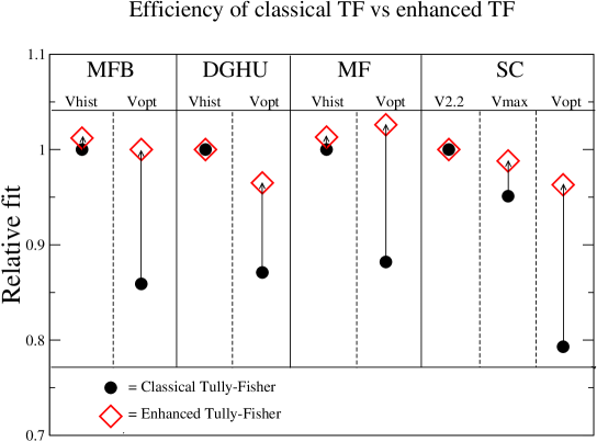
Figure 2:

The samples are given in the major columns and the major columns are subdivided according to which definition of $V_{rot}$ is used. The relative scaling-law performance is estimated using a normalized measure of the fit of the scaling law to the data, as follows:

• for each sample, the classical scaling law is calibrated using $V_{hist}$ in the case of MFB, MF and DGHU and $V_{2.2}$ in the case of SC;

• in each case, an estimate of fit to the data is given by the adjusted $R^{2}$ parameter, labelled $R_{MFB}^{2}$, $R_{MF}^{2}$, $R_{DGHU}^{2}$ and $R_{SC}^{2}$ respectively;

• each of $R_{MFB}^{2}$, $R_{MF}^{2}$, $R_{DGHU}^{2}$ and $R_{SC}^{2}$ is normalized to unity;

• for every other calibration of either the classical scaling law or the enhanced scaling law, the corresponding estimate of fit, $R^{2}$, is normalized using one of $R_{MFB}^{2}$, $R_{MF}^{2}$, $R_{DGHU}^{2}$ and $R_{SC}^{2}$, as appropriate.

In figure 2, the filled circles respresent the normalized $R^{2}$ values arising from the classical scaling law whilst the open diamonds represent these values arising from the enhanced scaling law. The figure makes it very clear that the effectiveness of the enhanced scaling-law is very much less sensitive to the definition of $V_{rot}$ than that of the classical scaling law. In particular:

• in every case, $V_{rot}=V_{opt}$ performs poorly in the classical scaling law but performs comparably with all other choices in the enhanced scaling law;

• for the DGHU and SC samples, the choices $V_{hist}$ and $V_{2.2}$ respectively appear to be optimal in the sense that the use of the enhanced scaling law makes no measurable difference over the classical scaling law;

• for the MFB and MF samples, the enhanced scaling law gives measurable, but small, improvements over the classical scaling law when $V_{hist}$ is used. The detailed analysis, given in the appendices, shows that these improvements are strongly significant in a statistical sense;

• for the SC sample, the enhanced scaling law gives much larger measurable improvement over the classical scaling law when $V_{2.2}$ is used.

4.3 Interim conclusions

We have demonstrated that the inclusion of the predictor $\alpha\log V_{rot}$ has the potential to greatly improve the predictive power of the Tully-Fisher scaling law but that, in practice, improvements are strongly contingent of the precise definition of $V_{rot}$ employed. It appears that there is an optimal definition of $V_{rot}$ which is similar to those employed by DGHU and SC but, whichever definition is used, suboptimal choices are brought to near-optimality by the inclusion of $\alpha\log V_{rot}$ as a predictor.

5 The classical Tully-Fisher scaling law

So far, we have shown that new insights into scaling laws for galaxy discs arise when we assume that $V\approx AR^{\alpha}$ over some partition of galaxy discs, $R_{min}<R<R_{max}$ say. In the following, we:

1. show how the Tully-Fisher scaling law emerges from the power-law hypothesis for the annular disc;

2. clarify why $\alpha\ln V_{rot}$ can be expected to be a significant predictor according to the precise definition chosen for $V_{rot}$.

5.1 The power-law hypthesis and the Tully-Fisher scaling law

Given the hypothesis $V=AR^{\alpha}$ for the rotation velocity in the annular disc, where $(A,\alpha)$ vary between discs, then for an arbitrarily chosen point $\left(R_{0},V_{0}\right)$ on any given rotation curve, we have

$$\ln A=\ln V_{0}-\alpha\ln R_{0}.$$ (5)

But we know that if, for example, we choose $V_{0}=V_{rot}$ on any given ORC then correlations of the type $V_{0}\equiv V_{rot}=f(M,\alpha)$ exist.

In practice, an exploration of the MFB, MF, DGHU and SC samples (see §6 for the quantitative numerical details) shows that models of the general type

$$\ln A\approx\left[\ln A\right]_{model}\equiv a_{0}+a_{1}M+\alpha\left(b_{1}+b_{2}M+b_{3}\ln S\right),$$ (6)

where $S$ is the surface brightness, are comprehensive (that is, all significant predictors are included) and account for, typically, 95% of the variation in $\ln A$ data.

A quick comparison of (5) with (6) shows that the decomposition

$$\ln V_{0}=a_{0}+a_{1}M,\,\,\,\ln R_{0}=-\left(b_{1}+b_{2}M+b_{3}\ln S\right)$$ (7)

is possible so that, immediately, we have the classical Tully-Fisher scaling law, together with a corresponding relation giving the value of $R\equiv R_{0}$ at which $V_{0}$ is measured. However, the decomposition (7) is not unique and in this observation we find an understanding of the appearance of $\alpha\ln V_{rot}$ as a predictor.

5.2 The predictor $\alpha\ln V_{rot}$ in the Tully-Fisher scaling law

The considerations of §5.1 above lead to an understanding of why $\alpha\ln V_{rot}$ is also a predictor in Tully-Fisher calibrations, and of why its significance varies according to the definition of $V_{rot}$ employed.

In effect, (7) defines both a particular characteristic velocity on an ORC and the characteristic radius at which this velocity is to be measured, both being determined in terms of luminosity properties of the galaxy concerned. However, suppose that we wish to defined the characteristic velocity at

$$\ln\hat{R}_{0}\equiv\ln R_{0}+\Delta\ln R_{0}$$

rather than at $\ln R_{0}$. Then (7) shows that, since $M$ and $S$ are fixed for the galaxy, $\Delta\ln R_{0}\neq 0$ can only arise from some perturbation of $(b_{1},b_{2},b_{3})$ - for example, $\Delta\ln R_{0}=-\Delta b_{2}M$. In this case, (5) can only be satisfied if (7) becomes

$$\ln\hat{V}_{0}=a_{0}+\left(a_{1}-\alpha\Delta b_{2}\right)M,\,\,\,\ln\hat{R}_{0}=-\left(b_{1}+b_{2}M+\Delta b_{2}M+b_{3}\ln S\right).$$

Thus, the simple act of redefining the characteristic radius according to $R_{0}\rightarrow\hat{R}_{0}$ immediately causes $\alpha\ln\hat{V}_{0}$ to become a predictor for $M$.

In other words, whether or not $\alpha\ln V_{0}$ is a significant predictor in any given case depends entirely upon the definition adopted for $V_{0}$ which, in effect, amounts to systematically selecting a particular definition for $R_{0}$.

6 The detailed analysis of the four samples

In the following, we show how the considerations of the previous section work in practice in the context of the samples of MFB, MF, SC and DGHU: in particular, we explore the model

$$\ln A\approx\left[\ln A\right]_{model}\equiv a_{0}+a_{1}M_{TF}+\alpha\left(b_{1}+b_{2}M_{TF}+b_{3}\ln S_{TF}\right)$$ (8)

for those samples where, in each case, $M_{TF}$ is estimated using Tully-Fisher relationships calibrated by the authors concerned.

6.1 The sample of MFB

The MFB sample contains 864 ORCs that we were able to fold and, after removing 28 of the more extreme outliers, the model (8) is defined by the table:

Coeffs	$a_{0}$	$a_{1}$	$b_{1}$	$b_{2}$	$b_{3}$	$R_{adj}^{2}$
Estimate	-0.946	-0.286	5.590	0.475	0.586	$95\%$
Std Error	0.149	0.007	0.286	0.015	0.020
$t$-statistic	-6	-41	20	31	29

so that, from (7) we immediately get

$$\ln V_{0}=-0.946-0.286M_{TF},\,\,\,\,\ln R_{0}=-5.590-0.475M_{TF}-0.586\ln S_{TF}.$$ (9)

The first of these two relations gives, directly (to two decimal places)

$$M_{TF}=-8.05\log_{10}V_{0}-3.31$$

which is very close to MFB’s calibration of the Tully-Fisher relation,

$$M_{TF}=-7.96\log_{10}V_{rot}-3.30.$$

6.2 The sample of MF

The MF sample contains 1083 ORCs that we were able to fold and, after removing 26 of the more extreme outliers, the model (8) is defined by the table:

Coeffs	$a_{0}$	$a_{1}$	$b_{1}$	$b_{2}$	$b_{3}$	$R_{adj}^{2}$
Estimate	-1.199	-0.298	5.976	0.469	0.477	$94\%$
Std Error	0.141	0.007	0.288	0.015	0.019
$t$-statistic	-9	-45	21	32	25

so that, from (7) we immediately get

$$\ln V_{0}=-1.199-0.298M_{TF},\,\,\,\,\ln R_{0}=-5.976-0.469M_{TF}-0.477\ln S_{TF}.$$ (10)

The first of these two relations gives, directly (to two decimal places)

$$M_{TF}=-7.45\log_{10}V_{0}-4.62$$

which is to be compared with MF’s (MFB’s) calibration of the Tully-Fisher relation,

$$M_{TF}=-7.96\log_{10}V_{rot}-3.30.$$

6.3 The sample of DGHU

The DGHU sample contains 497 ORCs that we were able to fold and, after removing 24 of the more extreme outliers, the model (8) is defined by the table:

Coeffs	$a_{0}$	$a_{1}$	$b_{1}$	$b_{2}$	$b_{3}$	$R_{adj}^{2}$
Estimate	-1.412	-0.307	5.540	0.434	0.415	$96\%$
Std Error	0.180	0.008	0.420	0.021	0.024
$t$-statistic	-8	-37	13	20	17

so that, from (7) we immediately get

$$\ln V_{0}=-1.412-0.307M_{TF},\,\,\,\,\ln R_{0}=-5.540-0.434M_{TF}-0.415\ln S_{TF}.$$ (11)

The first of these two relations gives, directly (to two decimal places)

$$M_{TF}=-7.50\log_{10}V_{0}-4.60$$

which is to be compared with DGHU’s calibration of the Tully-Fisher relation,

$$M_{TF}=-7.68\log_{10}V_{rot}-4.23.$$

6.4 The sample of SC using $V_{max}$

The SC sample contains 282 ORCs that we were able to fold and, after removing 24 of the more extreme outliers, the model (8) is defined by the table:

Coeffs	$a_{0}$	$a_{1}$	$b_{1}$	$b_{2}$	$b_{3}$	$R_{adj}^{2}$
Estimate	-3.225	-0.394	9.282	0.604	0.288	$98\%$
Std Error	0.219	0.010	0.744	0.0235	0.026
$t$-statistic	-15	-39	12	17	11

so that, from (7) we immediately get

$$\ln V_{0}=-3.225-0.394M_{TF},\,\,\,\,\ln R_{0}=-9.282-0.604M_{TF}-0.288\ln S_{TF}.$$ (12)

The first of these two relations gives, directly (to two decimal places)

$$M_{TF}=-5.84\log_{10}V_{0}-8.19$$

which is to be compared with SC’s calibration of the Tully-Fisher relation using his $V_{max}$,

$$M_{TF}=-6.19\log_{10}V_{rot}-7.50.$$

7 A quantitative test of the power-law hypothesis

So far, the assumption of the power-law hypothesis, $V_{rot}=AR^{\alpha}$, has led to considerable new insight into the scaling properties of galaxy discs so that ipso facto the hypothesis has great utility in practice; however, these results amount to qualitative evidence in favour of the hypothesis.

In the following we give a quantitative data analysis which shows that, at the level of statistical certainty, rotation velocities within the annular disc (defined in §3) of spirals behave as if the power law hypothesis

$$\left(\frac{V}{V_{0}}\right)\approx\left(\frac{R}{R_{0}}\right)^{\alpha},\,\,\,R_{min}<R<R_{max}\,,$$

where $\left(\alpha,V_{0},R_{0}\right)$ are parameters unique to each galaxy, is the physical law governing rotation velocity within spiral discs.

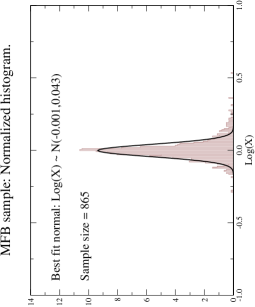
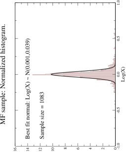
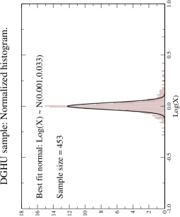
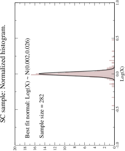
Figure 3: Distributions of $\log X$ for each of four large ORC samples.

7.1 The analysis

Any rotation curve can be expressed as

$$\left(\frac{V}{V_{0}}\right)=\left(\frac{R}{R_{0}}\right)^{\alpha}+g\left(\frac{R}{R_{0}}\right)$$ (13)

for arbitrary $\left(R_{0}>0,\,V_{0}>0,\,\alpha\right)$ and a suitably chosen function, $g\left(R/R_{0}\right)$. From this there follows immediately

$$\left(\frac{V}{V_{0}}\right) = \left(\frac{R}{R_{0}}\right)^{\alpha}\left[1+\left(\frac{R_{0}}{R}\right)^{\alpha}g\left(\frac{R}{R_{0}}\right)\right]\equiv\left(\frac{R}{R_{0}}\right)^{\alpha}X$$

$$\downarrow$$

$$\log\left(\frac{V}{V_{0}}\right) = \alpha\log\left(\frac{R}{R_{0}}\right)+\log X\,.$$ (14)

In the following, we show that, on the basis of the four large samples, $X=1$ in a statistical sense. The analysis proceeds as follows:

• choose the scaling functions relating $\left(V_{0},R_{0}\right)$ to luminosity properties, as one of (9), (10), (11) or (12) depending on the ORC sample being considered;

• with the chosen scaling functions, perform a linear regression of $\log\left(V/V_{0}\right)$ on $\log\left(R/R_{0}\right)$ as described in §3.1;

• we now have a linear model for (14) for the chosen ORC where the gradient gives an estimate of $\alpha$ and the zero point represents the $\log X$ term.

• the normalized histograms of the $\log X$ distributions, together with the best fitting pdf, is given in figure 2. For each of the four samples, the best pdf fits are given in the table:

Sample	$N(\bar{x},\sigma)$ fitted to $\log X$
MFB	$N(-0.001,0.043)$
MF	$N(+0.001,0.039)$
SC	$N(+0.002,0.026)$
DGHU	$N(+0.001,0.033)$

• It follows from the latter table and (14) that $X=1$ in the statistical sense, and at the level of near statistical certainty. In other words, there is absolutely no evidence to suggest that the power-law hypothesis for rotation velocities in the annular disc is not supported and that, for all practical purposes, we have

  $$\left(\frac{V}{V_{0}}\right)\approx\left(\frac{R}{R_{0}}\right)^{\alpha},\,\,\,R\in{\rm annular\,disc}\,$$

  for the annular disc in each of the four samples analysed.

8 Conclusions

It has been shown, at the level of statistical certainty, that:

• the optical disc of spiral galaxies consists of two quite distinct dynamical regions comprising an interior central sub-disc and a surrounding annular disc with an objectively defined dynamical transition boundary separating the two regions;

• that a scaling law, similar to the classical Tully-Fisher scaling law, applies on the interior boundary of the annular disc.

Furthermore, the analysis has provided a refinement of the Tully-Fisher scaling law, involving an additional parameter, which renders it insensitive to the precise definition of (optical) rotation velocity employed.

Appendix A The samples of MF and SC and $\alpha\log V_{rot}$

In the following, we describe the analyses corresponding to that of §4 applied to the samples of Mathewson & Ford, and Courteaux. For each sample, we use two definitions of $V_{rot}$:

• $V_{rot}=V_{author}$;

• $V_{rot}=V_{opt}$ defined as the rotational velocity estimated at $R_{83}$.

For each sample, we find that the use of $V_{opt}$ in the classical Tully-Fisher scaling law gives very significantly worse results that the use of $V_{author}$. However, we then find that performance of the enhanced Tully-Fisher law (with $\alpha\log V_{rot}$) is insensitive to the precise definition used of $V_{rot}$ with, for example, $V_{opt}$ being comparable to $V_{author}$ for overall effectiveness.

A.1 Sample of MFB using $V_{rot}=V_{hist}$

It is clear from their paper that MFB estimated $V_{rot}$ for their Tully-Fisher work using a version of the histogram method, but it is not clear, either from their words or their data, exactly how they implimented the method in practice. In the following, we calibrate the basic Tully-Fisher law using MFB’s estimates for $V_{rot}$ and absolute magnitudes, $M_{H}$ say, calculated from Hubble distances with $H=85km/sec/kpc$.

The classical Tully-Fisher scaling law with $V_{rot}=V_{hist}$

We find, for the classical Tully-Fisher model,

$$M_{H}\approx M_{TF} = (-6.72\pm 0.21)+(-6.54\pm 0.10)\log V_{rot};$$

$$(n=837,\,\,\,t_{grad}=-69)$$

$$Adj\,R^{2}=85\%,\,\,\,RSE=0.45$$

after removing 26 of the most extreme outliers. The quoted $t$-statistic refers to the gradient estimate. We note that the gradient lies well within the accepted envelope.

The enhanced Tully-Fisher scaling law with $V_{rot}=V_{hist}$

We find, for the enhanced model, using exactly the same reduced data set,

$$M_{H}\approx M_{TF} = (-7.47\pm 0.23)+\left[\left(-6.28\pm 0.10\right)+\left(0.22\pm 0.03\right)\alpha\right]\log V_{rot};$$

$$(n=837,\,\,\,t_{grad}=-62,\,\,\,t_{\alpha}=6.5)$$

$$Adj\,R^{2}=86\%,\,\,\,RSE=0.44$$

so that, according to the $t$-statistic for the gradient of the $\alpha\log V_{rot}$ component ($t_{\alpha}=6.5$), this component appears to be present in the model in a highly significant way. However, each model explains about $85\%$ of the variation in the data so that the inclusion of $\alpha$ does not make much difference to model’s predictive power in this case.

A.2 Sample of MFB using $V_{rot}=V_{opt}$

In the following we show that, for the MFB sample, $V_{rot}=V_{opt}$ performs poorly compared to MFB’s own determination, $V_{rot}=V_{hist}$, but that when $\alpha$ is included as a predictor, the enhanced model (using $V_{rot}=V_{opt}$) is directly comparable to models (A.1) and (A.1) above.

The classical Tully-Fisher scaling law with $V_{rot}=V_{opt}$

We find

$$M_{H}\approx M_{TF} = (-7.70\pm 0.28)+(-5.98\pm 0.13)\log V_{opt};$$

$$(n=837,\,\,\,t_{grad}=-47)$$

$$Adj\,R^{2}=73\%,\,\,\,RSE=0.60$$

after removing twelve of the most extreme outliers. The quoted $t$-statistic refers to the gradient estimate. Note that this model explains only about 73% of the variation in the data compared to about 85% for model (A.1) above.

The enhanced Tully-Fisher scaling law with $V_{rot}=V_{opt}$

Using exactly the same reduced data set as above, we find

$$M_{H}\approx M_{TF} = (-8.88\pm 0.22)+\left[\left(-5.73\pm 0.10\right)+\left(0.78\pm 0.03\right)\alpha\right]\log V_{opt};$$

$$(n=837,\,\,\,t_{grad}=-57,\,\,\,t_{\alpha}=26)$$

$$Adj\,R^{2}=85\%,\,\,\,RSE=0.45.$$

It is clear that the $\alpha\log V_{opt}$ component ($t_{\alpha}=26$) is very powerfully present in the model. Furthermore, this model now explains about $85\%$ of the variation in the data (up from 73%) and so is directly comparable with models (A.1) and (A.1) which both use MFB’s own $V_{rot}=V_{hist}$ determinations.

A.3 Sample of Dale et al using $V_{rot}=V_{hist}$

The primary conclusion from the foregoing analysis of MFB data is that the inclusion of the predictor $\alpha\ln V_{rot}$ significantly enhances the performance of the Tully-Fisher scaling law. However, it transpires that the degree of this enhancement depends on the precise definition of $V_{rot}$ employed, as we now demonstrate via the analysis of the DGHU data.

The classical Tully-Fisher scaling law with $V_{rot}=V_{hist}$

If we calibrate the basic Tully-Fisher law using Dale’s own estimates ($0.5\left(V_{90\%}-V_{10\%}\right)$) for $V_{rot}$ and absolute magnitudes calculated from Hubble distances with $H=85km/sec/kpc$ we find, for the TF classical model,

$$M_{TF} = (-7.18\pm 0.28)+(-6.48\pm 0.13)\log V_{rot};\,\,\,(n=478,\,\,\,t=-52)$$

$$Adj\,R^{2}=85\%,\,\,\,RSE=0.40$$

after removing eighteen of the most extreme outliers. The quoted $t$-statistic refers to the gradient estimate. We note that the gradient lies well within the accepted envelope.

The enhanced Tully-Fisher scaling law with $V_{rot}=V_{hist}$

We find, for the enhanced model, using exactly the same reduced data set:

$$M_{TF} = (-7.39\pm 0.31)+\left[\left(-6.41\pm 0.14\right)+\left(0.07\pm 0.04\right)\alpha\right]\log V_{rot};$$

$$(n=478,\,\,\,t_{grad}=-47,\,\,\,t_{\alpha}=1.5)$$

$$Adj\,R^{2}=85\%,\,\,\,RSE=0.40$$

so that, according to the $t$-statistic for the gradient of the $\alpha\log V_{rot}$ component ($t_{\alpha}=1.5$), this component appears to be not significantly present in the model.

A.4 Sample of Dale using $V_{rot}=V_{opt}$

To emphasize the point that it is Dale’s definition of $V_{rot}$ which makes $\alpha\log V_{rot}$ insignificant, rather than some property of the sample, we repeat the analysis of DGHU data, but using $V_{rot}\equiv V_{opt}$.

The classical Tully-Fisher scaling law with $V_{rot}=V_{opt}$

We find, for the classical TF model using $V_{opt}=V(R_{83})$,

$$M_{TF} = (-7.54\pm 0.38)+(-6.22\pm 0.17)\log V_{opt};\,\,\,(n=477,\,\,\,t=-37)$$

$$Adj\,R^{2}=74\%,\,\,\,RSE=0.53$$

after removing eighteen of the most extreme outliers. The quoted $t$-statistic refers to the gradient estimate. We note that this model is considerably less effective in explaining the data than when $V_{rot}=V_{hist}$ is used.

The enhanced Tully-Fisher scaling law with $V_{rot}=V_{opt}$

For the enhanced model, we find

$$M_{TF} = (-8.40\pm 0.32)+\left[\left(-6.01\pm 0.14\right)+\left(0.61\pm 0.04\right)\alpha\right]\log V_{opt};$$

$$(n=478,\,\,\,t_{grad}=-43,\,\,\,t_{\alpha}=15)$$

$$Adj\,R^{2}=82\%,\,\,\,RSE=0.44$$

so that, according to the $t$-statistic for the gradient of the $\alpha\log V_{rot}$ component ($t_{\alpha}=15$), this component appears to be present in the model in an extremely significant way. Furthermore, the inclusion of the predictor $\alpha\log V_{rot}$ has sufficiently enhanced the predictive power of the model so that it is comparable with the model which uses $V_{rot}=V_{hist}$.

A.5 Sample of MF using $V_{rot}=V_{hist}$

The classical Tully-Fisher scaling law with $V_{rot}=V_{hist}$

If we calibrate the basic Tully-Fisher law using MF’s own estimates for $V_{rot}$ and absolute magnitudes calculated from Hubble distances with $H=85km/sec/kpc$ we find, for the classical TF model,

$$M_{TF} = (-9.23\pm 0.21)+(-5.50\pm 0.10)\log V_{rot};\,\,\,(n=1057,\,\,\,t=-58)$$

$$Adj\,R^{2}=76\%,\,\,\,RSE=0.46$$

after removing 28 of the most extreme outliers. The quoted $t$-statistic refers to the gradient estimate. We note that the gradient is on the low side of expected values.

The enhanced Tully-Fisher scaling law with $V_{rot}=V_{hist}$

We find, for the enhanced model, using exactly the same reduced data set,

$$M_{TF} = (-9.88\pm 0.23)+\left[\left(-5.27\pm 0.10\right)+\left(0.21\pm 0.03\right)\alpha\right]\log V_{rot};$$

$$(n=1057,\,\,\,t_{grad}=-53,\,\,\,t_{\alpha}=6.6)$$

$$Adj\,R^{2}=77\%,\,\,\,RSE=0.46$$

so that, according to the $t$-statistic for the gradient of the $\alpha\log V_{rot}$ component ($t_{\alpha}=6.6$), this component appears to be present in the model in a highly significant way.

We see that the inclusion of the predictor $\alpha\ln V_{rot}$ gives a significant, but small, improvement in performance.

A.6 Sample of MF using $V_{rot}=V_{opt}$

The classical Tully-Fisher scaling law with $V_{rot}=V_{opt}$

If we calibrate the basic Tully-Fisher law using $V_{opt}\equiv V(R_{83})$ we find, for the classical TF model,

$$M_{TF} = (-9.83\pm 0.25)+(-5.11\pm 0.11)\log V_{opt};\,\,\,(n=1053,\,\,\,t=-47)$$

$$Adj\,R^{2}=67\%,\,\,\,RSE=0.54$$

after removing 32 of the most extreme outliers. We see that the model explains about 67% of the variation in the data, compared with about 76% for model (A.5). It is thus very much less effective.

The enhanced Tully-Fisher scaling law with $V_{rot}=V_{opt}$

However, if we now consider the enhanced model, we find

$$M_{TF} = (-10.49\pm 0.20)+\left[\left(-5.04\pm 0.09\right)+\left(0.61\pm 0.03\right)\alpha\right]\log V_{opt};$$

$$(n=1053,\,\,\,t_{grad}=-56,\,\,\,t_{\alpha}=23)$$

$$Adj\,R^{2}=78\%,\,\,\,RSE=0.44$$

so that, according to the $t$-statistic for the gradient of the $\alpha\log V_{rot}$ component ($t_{\alpha}=23$), this component is very powerfully present in the model. Furthermore, the model now explains about 78% of the variation in the data and is therefore significantly better than model (A.5) which uses MF’s own estimate of $V_{rot}$.

A.7 Sample of SC using $V_{rot}=V_{model}\equiv V_{max}$

Courteaux’s paper is primarily a study of various methods of estimating $V_{rot}$ for Tully-Fisher studies and his estimator $V_{max}$ is derived from as the peak velocity achieved by a particular phenomenological model.

The classical Tully-Fisher scaling law with $V_{rot}=V_{max}$

If we calibrate the basic Tully-Fisher law using Courteaux’s $V_{max}$ and absolute magnitudes calculated from Hubble distances with $H=85km/sec/kpc$ we find, for the classical TF model,

$$M_{TF} = (-5.53\pm 0.50)+(-6.66\pm 0.22)\log V_{rot};\,\,\,(n=254,\,\,\,t=-30)$$

$$Adj\,R^{2}=78\%,\,\,\,RSE=0.39$$

after removing twenty of the most extreme outliers. The quoted $t$-statistic refers to the gradient estimate. We note that the gradient lies well within the accepted envelope.

The enhanced Tully-Fisher scaling law with $V_{rot}=V_{max}$

We find, for the enhanced model, using exactly the same data set

$$M_{TF} = (-6.85\pm 0.52)+\left[\left(-6.17\pm 0.22\right)+\left(0.36\pm 0.06\right)\alpha\right]\log V_{rot};$$

$$(n=254,\,\,\,t_{grad}=-28,\,\,\,t_{\alpha}=5.9)$$

$$Adj\,R^{2}=81\%,\,\,\,RSE=0.36$$

so that, according to the $t$-statistic for the gradient of the $\alpha\log V_{rot}$ component ($t_{\alpha}=6.3$), this component appears to be present in the model in a highly significant way.

A.8 Sample of SC using $V_{rot}=V_{model}\equiv V_{2.2}$

Courteaux’s paper is primarily a study of various methods of estimating $V_{rot}$ for Tully-Fisher studies and his estimator $V_{2.2}$ is the model velocity at $2.15\times$scale lengths.

The classical Tully-Fisher scaling law with $V_{rot}=V_{2.2}$

If we calibrate the basic Tully-Fisher law using Courteaux’s $V_{2.2}$ and absolute magnitudes calculated from Hubble distances with $H=85km/sec/kpc$ we find, for the classical TF model,

$$M_{TF} = (-6.43\pm 0.41)+(-6.33\pm 0.18)\log V_{rot};\,\,\,(n=262,\,\,\,t=-34)$$

$$Adj\,R^{2}=82\%,\,\,\,RSE=0.36$$

after removing eighteen of the most extreme outliers. The quoted $t$-statistic refers to the gradient estimate. We note that the gradient lies well within the accepted envelope.

The enhanced Tully-Fisher scaling law with $V_{rot}=V_{2.2}$

We find, for the enhanced model, using exactly the same data set

$$M_{TF} = (-6.83\pm 0.47)+\left[\left(-6.18\pm 0.20\right)+\left(0.10\pm 0.06\right)\alpha\right]\log V_{rot};$$

$$(n=262,\,\,\,t_{grad}=-31,\,\,\,t_{\alpha}=1.8)$$

$$Adj\,R^{2}=82\%,\,\,\,RSE=0.36$$

so that, according to the $t$-statistic for the gradient of the $\alpha\log V_{rot}$ component ($t_{\alpha}=6.3$), this component appears to be present in the model in a highly significant way.

A.9 Sample of SC using $V_{rot}=V_{opt}$

The classical Tully-Fisher scaling law with $V_{rot}=V_{opt}$

If we calibrate the basic Tully-Fisher law using Courteaux’s $V_{opt}$ and absolute magnitudes calculated from Hubble distances with $H=85km/sec/kpc$ we find, for the classical TF model,

$$M_{TF} = (-6.59\pm 0.64)+(-6.12\pm 0.28)\log V_{opt};\,\,\,(n=254,\,\,\,t=-22)$$

$$Adj\,R^{2}=65\%,\,\,\,RSE=0.49$$

after removing 21 of the most extreme outliers. The quoted $t$-statistic refers to the gradient estimate. We note that the gradient lies well within the accepted envelope.

The enhanced Tully-Fisher scaling law with $V_{rot}=V_{opt}$

For the enhanced model, we find

$$M_{TF} = (-7.84\pm 0.51)+\left[\left(-5.76\pm 0.22\right)+\left(0.75\pm 0.06\right)\alpha\right]\log V_{opt};$$

$$(n=254,\,\,\,t_{grad}=-26,\,\,\,t_{\alpha}=13)$$

$$Adj\,R^{2}=79\%,\,\,\,RSE=0.38$$

so that, according to the $t$-statistic for the gradient of the $\alpha\log V_{rot}$ component ($t_{\alpha}=134$), this component is present in the model in an extremely significant way.

References

- [1942] Danver, C.G., Lund Obs, Ann., Vol 10
- [1981] Kennicutt, R.C., 1981, AJ, 86, 1847
- [1997] Courteau S., 1997, AJ, 114, 6, 2402-2427
- [1997] Dale DA, Giovanelli R, Haynes M, 1997 AJ 114 (2): 455-473
- [1998] Dale DA, Giovanelli R, Haynes MP, Scodeggio M, Hardy E, Campusano LE, 1998 AJ 115 (2), 418-435
- [1999] Dale D.A., Giovanelli R, Haynes M.P., 1999, AJ 118 (4), 1468-1488
- [2000] Dale D.A., Uson JM, 2000, AJ 120 (2), 552-561
- [2001] Dale D.A., Giovanelli R, Haynes M.P., Hardy E, Campusano LE, 2001, AJ 121, 1886-1892
- [1997] Giovanelli R., Haynes M.P., Herter T., Vogt N.P., da Costa L.N., Freudling W., Salzer J.J., Wegner G. 1997 AJ 113 (1), 53
- [1992] Mathewson D.S., Ford V.L., Buchhorn M. 1992, ApJS 81 413
- [1996] Mathewson D.S., Ford V.L. 1996, ApJS 107 97
- [1996] Persic M., Salucci P., Stel F., 1996, MNRAS 281 27
- [1991] Persic M., Salucci P., 1991, ApJ 368 60
- [1995] Persic M., Salucci P., 1995, ApJS 99 501
- [1999a] Roscoe D.F., 1999a, A&A,343, 697-704
- [1999b] Roscoe D.F., 1999b, A&A,343, 788-800
- [1999c] Roscoe D.F., 1999c, A&AS,140, 247-260
- [1980] Rubin V.C., Ford W.K., Thonnard N. 1980, ApJ 238 471