Numerical simulation evidence of spectrum rearrangement in impure graphene

Abstract

By means of numerical simulation we confirm that in graphene with point defects a quasigap opens in the vicinity of the resonance state with increasing impurity concentration. We prove that states inside this quasigap cannot longer be described by a wavevector and are strongly localized. We visualize states corresponding to the density of states maxima within the quasigap and show that they are yielded by impurity pair clusters.

I Introduction

Not so long ago, graphene has been cleaved out for the first time by the so–called scotch–tape technique.Novo Since that, this novel, truly two–dimensional material continues to put new challenges to scientific community. Graphene is already known to manifest some remarkable properties. The most unusual of them, and, correspondingly, the most frequently emphasized on, is the Dirac dispersion of Fermi elementary excitations. This unusual spectrum makes graphene a rather promising material for a variety of applications in computer electronics and chemical sensors. While graphene is known to possess outstanding structural stability and crystalline quality, existing methods of its isolation necessarily imply the presence of a certain amount of defects. Moreover, impurities can be embedded into graphene intentionally in order to tune up its physical characteristics in accordance with a specific application. Even though some applications are destined for a distant future, the need in deliberate and proper functionalization of graphene provides adequate grounds for an extensive study of different types of defects in this material. Despite a noticeable quantity of papers devoted to the study of impure graphene, a comprehensive understanding of impurity effects on its electron spectrum is still lacking.

While different types of disorder are inherent in graphene, below we are particularly interested among them in the substitutional point defects. This commonly used model applies not only to chemically substituted carbon atoms or an absence of them (vacancies), but also, to a known extent, to adsorbed atoms, molecules, or radicals on the graphene sheet.adatoms Regarding the substitutional impurities in graphene, comprehensive attention has been paid as to the single impurity problem, in which the impurity state wave function has been studied for a single defect and a pair of them,Katsnelson as to the evolution of the density of states (DOS) in graphene with increasing the impurity concentration.Pereira1 ; Pereira2 ; Sarma ; Pereira ; Wu However, such a phenomenon as spectrum rearrangement is frequently overlooked. The main concept of the spectrum rearrangement is based on the existence of some critical impurity concentration, at which the spectrum of a disordered system undergoes a cardinal qualitative change. As a rule, the spectrum rearrangement should be related to the appearance of a local level or a resonance state. Characteristics of this impurity state, namely its energy and damping, which are determined within the single impurity problem, are shaping the scenario and type of the subsequent spectrum rearrangement. Albeit a single point defect is expected to perturb only the lattice cite occupied by an impurity or, at most, the adjacent lattice cites, and thus should be classified as a short-range defect, the effective radius of the correspondent impurity state can far exceed the lattice constant, when its energy is close to the van Hove singularity in the spectrum. Spacial overlap of individual impurity states, which occurs with increasing the impurity concentration, is marking the onset of the spectrum rearrangement. This simple consideration gives a possibility to roughly estimate the critical concentration of the spectrum rearrangement. Since the effective radius of the single impurity state in certain cases can be large compared to the lattice constant, the respective critical concentration should be fairly low. As a result, in such situations only a trace amount of impurities can provoke the spectrum rearrangement.

In graphene, the spectrum rearrangement driven by an increase in the concentration of defects described by the Lifshitz model has been analytically examined in Refs. YuV, ; YuV0, . It has been demonstrated that the passage of the spectrum rearrangement is of the anomalous type due to a weak resonance state. That means that for a sufficiently large compared to the bandwidth impurity potential a quasigap is gradually opening around the resonance energy and at the critical concentration spans up to the Dirac point in the spectrum. With further increase in the impurity concentration (i.e. after the spectrum rearrangement), the quasigap is rapidly enlarging. In this regime the width of the quasigap is approximately proportional to the square root of the impurity concentration. In Refs. YuV, ; YuV0, the analysis of the spectrum rearrangement in graphene has been conducted by means of the coherent potential approximation (CPA) applicability criterion, which is instrumental in determining spectrum domains with different degree of localization.sprb

The aim of the current work is to carry out the numerical simulation of graphene DOS with the special emphasis on the spectrum rearrangement phenomenon (for its physical description see also the review Ref. ilp, ). By considering for each chosen perturbation strength those impurity concentrations that are close to the expected critical concentration of the spectrum rearrangement, we show that implementing the criterion of the CPA applicability it is possible to judge upon the spectrum rearrangement process in graphene. As a next step in our previous attempts,YuV ; YuV0 we are paying a special attention to the CPA validity. By comparing the CPA output with the numerical results, we verify that the CPA applicability criterion works rather well. We also notice that when impurity concentration is low enough, the average T-matrix approximation (ATA) is in good agreement with numerically calculated DOS. We discuss the spectrum rearrangement in graphene and the correspondent interplay between numerical and analytical results. After the spectrum rearrangement takes place, we identify the cluster structure of graphene’s DOS in the vicinity of the impurity resonance energy. The structure observed evidently cannot be explained by means of available analytic approaches and requires further analysis.

As an effective tool for numerical calculations we employ the negative eigenvalue theorem as suggested by Dean.Dean This approach, to the best of our knowledge, hasn’t been used for graphene yet (see, e.g. Refs. Pereira, ; Wu, ). Its advantages are discussed below. Finally, we describe a drift of the Fermi energy from the DOS minimum, a kind of a self–doping effect, when Fermi level shifts away without actual introduction of additional carriers into the disordered system.

The paper is organized as follows: in Section II A we remind the basic mathematical impurity model. In Section II B we introduce the concept of spectrum rearrangement. In Section II C we briefly set forth the numerical approach. In Section III we present and discuss results. In the last Section we summarize outcomes of our study.

II Model disordered system and methods of its analysis

II.1 Impurity model

In the tight–binding approximation the simplest (for spinless fermions) graphene Hamiltonian has the form,

$$\mathbf{H_{0}}=t\sum\limits_{<\bm{n}_{\alpha},\bm{m}_{\beta}>}\mathbf{a}_{\bm{n}_{\alpha}}^{\dagger}\mathbf{a}_{\bm{m}_{\beta}}.$$ (1)

Here, $t\approx 2.7eV$ is the hopping integral, $\bm{n}$ and $\bm{m}$ denote vectors of lattice cells, Greek indices $\alpha$ and $\beta$ correspond to the graphene sublattices, and summation runs over all nearest neighbors. It has been confirmed experimentally that this approximation describes graphene’s electronic spectrum fairly well.Bostwick

The diagonal element of the Green’s function in the cite representation,

$$g_{\bm{n}_{\alpha}\bm{m}_{\beta}}(\varepsilon)=\lim_{\delta\rightarrow 0^{+}}\sum\limits_{j}\frac{\psi_{\bm{n}_{\alpha}}(j)\psi^{{\dagger}}_{\bm{m}_{\beta}}(j)}{\varepsilon+i\delta-\varepsilon(j)},$$ (2)

where the summation runs over all eigenstates $\psi(j)$, and $\varepsilon(j)$ are their corresponding eigenvalues, in the case of Hamiltonian (1) can be easily approximated by

$$g_{0}(\varepsilon)=g_{0_{\alpha}0_{\alpha}}(\varepsilon)\approx\frac{2\varepsilon}{W^{2}}ln\left(\frac{|\varepsilon|}{W}\right)-i\pi\frac{|\varepsilon|}{W^{2}}$$ (3)

in the low–energy limit, i.e. $|\varepsilon|\ll W=\sqrt{\pi\sqrt{3}}t$, where $W$ is the bandwidth. A detailed derivation of (3) can be found in Refs. YuV, ; YuV0, . A comparison between the exact diagonal element of the Green’s function and its low–energy approximation is given in Fig. 1.

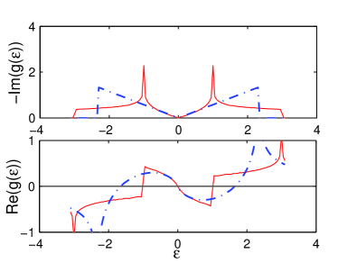
Figure 1: (color online) A comparison between the exact $g_{0}(\epsilon)$ (solid line) and its analytical approximation (3) (dash-dotted line).

Since we are interested only in the relatively close vicinity of the Dirac point in the spectrum, the approximation (3) looks appropriately shaped.

While the host DOS can be straightforwardly found from the imaginary part of the latter expression, impurities break the translational symmetry and so the DOS of disordered graphene (which is the focus of the current investigation) cannot be directly obtained. Point defects in graphene are usually modeled by adding the following perturbation in the Hamiltonian (the so–called Lifshitz model):

$$\mathbf{U}=V_{L}\sum\limits_{\bm{p}_{\alpha}}\mathbf{a}_{\bm{p}\alpha}^{\dagger}\mathbf{a}_{\bm{p}\alpha},$$ (4)

where $V_{L}$ is the impurity potential, and $\bm{p}_{\alpha}$ runs over sites occupied by impurities. It is supposed that impurities are distributed among lattice sites absolutely at random with concentration $c$ representing the probability that an arbitrary site is occupied by an impurity. Thus, for a large system with $N$ lattice sites the total amount of impurities tends to $cN$.

II.2 Spectrum rearrangement and CPA applicability criterion

When the impurity concentration is small enough, conventional analytic approachesElliot ; Lifhitz can be applied. To be concise, in the first approximation the averaged perturbed Green’s function

$$\mathbf{G}(\varepsilon)=<(\varepsilon-\mathbf{H_{0}-U})^{-1}>$$ (5)

can be found as some renormalization of the host Green’s function:

$$\mathbf{G}(\varepsilon)=\mathbf{g}(\varepsilon-\sigma(\varepsilon))$$ (6)

Two cases are of a particular interest: the average T-matrix approximation (ATA),

$$\sigma_{ATA}(\varepsilon)=\frac{cV_{L}}{1-(1-c)V_{L}g_{0}(\varepsilon)},$$ (7)

which accounts for multiple single–site scattering by an impurity, and the coherent potential approximation,

$$\sigma_{CPA}(\varepsilon)=\frac{cV_{L}}{1-[V_{L}-\sigma_{CPA}(\varepsilon)]g_{0}(\varepsilon-\sigma_{CPA}(\varepsilon))},$$ (8)

which adds the self–consistency. In the CPA the self–energy is taken from the requirement that the single–site renormalized T-matrix should be zero on average. In both methods scatterings on pairs and larger groups of impurities is omitted. Thus, these approximations are expected to remain valid, when cluster effects are insignificant in a disordered system.

However, when impurity concentration is gradually increased, individual impurity states (visualized for graphene, e.g., in Ref. Katsnelson, ) begin to overlap with each other. Thus, a contribution from scatterings on impurity clusters to the self–energy is becoming more pronounced in the vicinity of the impurity state energy. As a result, a significant overlap between impurity states corresponds to the commencement of substantial modifications in the spectrum of a disordered system. In other words, it points out the critical concentration of the spectrum rearrangement. This simple reasoning provides a possibility to estimate the critical concentration in graphene with Lifshitz impurities. From the expression for the non-diagonal element of the host Green’s function,Bena it can be deduced that an effective decay radius of the impurity state is $r_{imp}\approx|V_{L}|$. It should be noticed that in commonly encountered cases for the Lifshitz impurity model, an increase in the parameter $V_{L}$ leads to the intensification of the impurity state localization and, consequently, to a decrease in $r_{imp}$. The opposite result for graphene is caused by the particle–hole symmetry of the Dirac Hamiltonian. Another characteristic space interval is the average distance between impurities, which depends on impurity concentration as $<r>\sim 1/\sqrt{c}$. Both radii coincide ($<r>\approx r_{imp}$) at some impurity concentration $c_{r}\sim 1/V_{L}^{2}$. Thus, the condition $<r>\approx r_{imp}$ defines the spectrum rearrangement concentration $c_{r}$. As has been argued in Ref. YuV, , at this critical concentration a quasigap filled with strongly localized states should sweep from the resonance energy to the Dirac point, stimulating an accumulation of considerable changes in the DOS. Albeit this condition is reasonably intuitive, it is too rough for an accurate forecast of the critical concentration. Moreover, it does not provide any information on the energy intervals, in which the spectrum is more exposed to the rearrangement process. Since cluster effects, which make up the core of the spectrum rearrangement, are not included into the CPA, the CPA applicability criterion can be successfully employed for the analysis of the spectrum rearrangement process. This very approach has been in fact realized in Refs. YuV, ; YuV0, for the impure graphene. Namely, by following the conventional technique of the Green’s function cluster expansionilp ; Lifhitz it is possible to represent the self–energy as a series in all possible groups of impurity centers. At that, the first term of this series corresponds to the conventional CPA. The small parameter of the series,

$$R(\varepsilon)=\\ =\left|c\left[\frac{V_{L}-\sigma_{CPA}(\varepsilon)}{1-[V_{L}-\sigma_{CPA}(\varepsilon)]g_{0}(\varepsilon-\sigma_{CPA}(\varepsilon))}\right]^{2}+\right.\\ \left.+(1-c)\left[\frac{-\sigma_{CPA}(\varepsilon)}{1+\sigma_{CPA}(\varepsilon)g_{0}(\varepsilon-\sigma_{CPA}(\varepsilon))}\right]^{2}\right|\times\\ \times\left[\sum_{\bm{n}\neq 0}|g_{\bm{0}_{1}\bm{n}_{1}}(\varepsilon-\sigma_{CPA}(\varepsilon))|^{2}+\right.\\ +\left.\sum_{\bm{n}}|g_{\bm{0}_{1}\bm{n}_{2}}(\varepsilon-\sigma_{CPA}(\varepsilon))|^{2}\right],$$ (9)

is indicative of the relative strength of cluster effects at a given energy, and can be used to outline qualitatively different spectrum domains.

In those spectral domains, where the small parameter of the series $R(\epsilon)$ is high, the CPA is not reliable and correspondent states are showing a tendency towards localization. For ordinary 3D systems a mobility edge should be expected close to the energy, at which $R(\epsilon)=0.5$.sprb At the same time, it can be demonstrated that the maximum magnitude of $R(\epsilon)$ is unity, and it is reached at the van Hove singularities of the spectrum. At the low impurity concentration, expression (9) can be approximated by

$$R(\varepsilon)=\left|\frac{\sigma_{CPA}^{2}(\varepsilon)}{c}\left[g_{0}(E)+\frac{\partial g_{0}(E)}{\partial E}\right]_{E=\varepsilon-\sigma(\varepsilon)}\right|$$ (10)

There are two factors in (10). The first of them, $\sigma_{CPA}^{2}(\varepsilon)/c$, increases in absolute magnitude around the impurity state energy, which can be determined from the Lifshitz equation, $1=V_{L}g_{0}(\varepsilon)$). The second one (in the square brackets) is the sum of the Green’s function and its derivative, which increases in the vicinity of the Dirac point (or any other van Hove singularity). Consequently, the energy dependence of the CPA applicability criterion should possess different maxima, around which the CPA is not valid. Even though the CPA applicability criterion has been deduced for the fictitious system with a single Dirac cone in the spectrum, it will be apparent below that it is an adequate tool for the spectrum rearrangement analysis in the actual graphene. As regards the CPA and the ATA, it is not difficult to show that presence of the two different Dirac cones in graphene alters their output only in a trivial way.

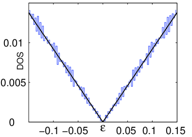
Figure 2: (color online) Density of states for graphene without impurities obtained by Dean’s numerical method compared to the exact one for the infinite system.

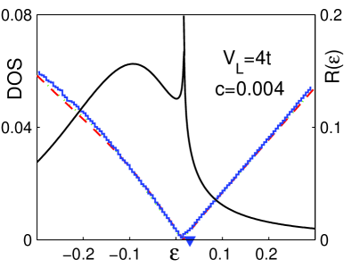
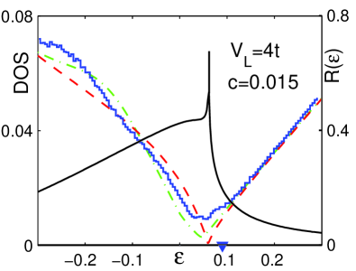
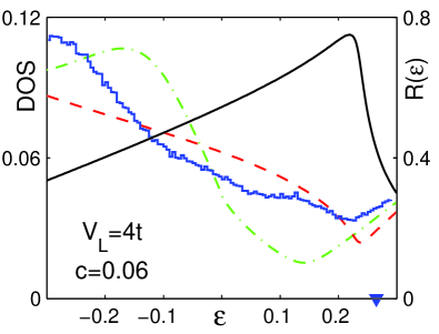
Figure 3: (color online) A set of figures corresponding to impurity perturbation $V_{L}=4t$ and different concentrations. Critical concentration is $c_{r}\approx 0.015$. Stepped curve stands for the numerical computation, dashed — the CPA, dash–dotted — the ATA (left Y-axis represents their values). Solid black curve is $R(\varepsilon)$ (right Y-axis represents its values). Triangle on the energy axis denotes the Fermi level position.

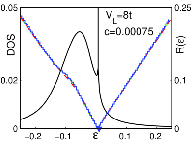
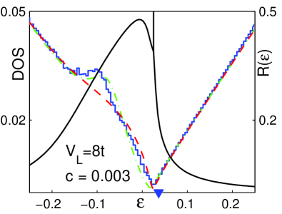
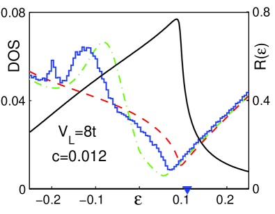
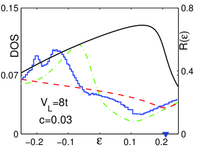
Figure 4: (color online) A set of figures corresponding to impurity perturbation $V_{L}=8t$ and different concentrations. Critical concentration is $c_{r}\approx 0.003$. Stepped curve stands for the numerical computation, Dashed — the CPA, dash–dotted — the ATA (left Y-axis represents their values). Solid black curve is $R(\varepsilon)$ (right Y-axis represents its values). Triangle on the energy axis denotes the Fermi level position.

II.3 Numerical method

Numerical techniques involving diagonalization of the random matrix are too resource consuming to simulate disordered systems approaching in their dimensions real experimental samples. However, information on eigenvectors is superficial for the DOS calculations. So far, the Haydock method,Haydock based on an expansion of the diagonal element of the Green’s function into an infinite fraction, has been extensively used for numerical calculation of the graphene DOS.Pereira ; Wu Still, this approach is not without its shortcomings. It is the local DOS (LDOS) that is calculated within this approach. The necessity to truncate the infinite fraction at some point sometimes leads to unphysical oscillations of the LDOS, which are difficult to keep under control and to distinguish from actual features of the spectrum. Furthermore, the total DOS is obtained in the Haydock method by averaging the LDOS at several lattice sites, and an inclusion of all sites in the model system into the averaging process is absolutely impractical. The above leaves a touch of uncertainty in the DOS minutiae. In a contrast, we relied on the Dean’s calculation scheme.Dean It allows to obtain the total number of eigenvalues of a hermitian matrix that are less than a specified value. This provides a possibility to explore the DOS with a desired degree of precision and to preserve all particularities of the resulting curve.

This method has proven to be especially effective for 1D systems. The time required to finish a single Dean’s algorithm loop is proportional to the number of atoms ($N$) in a 1D system, which is fast enough to simulate really large 1D systems. However, with an increase in the system’s dimensionality, the computational time required for one loop increases. For a 2D system it is proportional to $N^{2}$.Dean In our case of graphene, we obtained DOSs for the system comprised of $5.3\cdot 10^{6}$ atoms, which corresponds to a system with the linear dimensions about $0.3\mu m$ — about the size of real experimental samples. To eliminate the influence of boundary states on the DOS we applied periodical boundary condition for the zigzag boundary of the model system under consideration.zigzag The numerically calculated DOS for the described model system is given in Fig. 2. Some jaggedness seen in the DOS curve is related to the finite size of the model system.

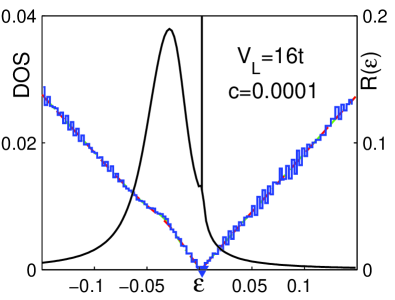
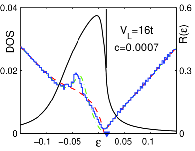
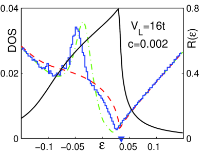
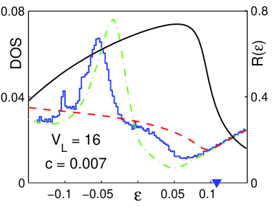
Figure 5: (color online) A set of figures corresponding to the impurity perturbation $V_{L}=16t$ and different concentrations. Critical concentration is $c_{r}\approx 0.0007$. Stepped curve stands for the numerical computation, dashed — the CPA, dash–dotted — the ATA (left Y-axis represents their values). Solid black curve is $R(\varepsilon)$ (right Y-axis represents its values). Triangle on the energy axis denotes the Fermi level position.

III Results and discussion

The figures Fig. 3, Fig. 4, and Fig. 5 correspond to impurity perturbations $V_{L}=4t$, $V_{L}=8t$, and $V_{L}=16t$, respectively. At the negative impurity potentials $V_{L}$ the whole picture is simply mirrored against the zero energy. For each perturbation magnitude we consider qualitatively different regions of impurity concentration: $c<c_{r}$ (before the spectrum rearrangement), $c\approx c_{r}$ (in the course of the spectrum rearrangement) and $c>c_{r}$ (after the spectrum rearrangement). We plot the CPA DOS, the ATA DOS, and the numerically calculated DOS, with the left Y-axis representing their values. We add the CPA applicability criterion by plotting the small parameter of the series $R(\varepsilon)$ (solid line), with the right Y-axis showing its values in the same figures. We also designated by the triangle the Fermi level position, obtained from the numerical data for the impure system.

For the low concentrations (i.e. those that are less than $c_{r}$), analytical curves, namely the CPA DOS and the ATA DOS, perfectly fit the numerical histogram. The DOS only slightly deviates from the conventional Dirac DOS mainly because of the shift towards positive energies. The applicability criterion $R(\varepsilon)<0.5$ is satisfied practically at all energies within the chosen window, $R(\varepsilon)$ is small and characteristically contains two maxima. The sharp one corresponds to the van Hove singularity and predicts failure of analytical approximations in the Dirac point vicinity. Less sharp one is due to the $\sigma^{2}$ factor.

When the impurity concentration is increased approximately to the critical value $c_{r}$, maxima of small parameter $R(\varepsilon)$ show the tendency to merge together into a single maximum, which height goes beyond the $0.5$ value (as it was shown in Ref. YuV, ). This event indicates the onset of the spectrum rearrangement, providing a reference point for the critical concentration at the given $V_{L}$. In the domain with heightened values of $R(\varepsilon)$ the discrepancy between the CPA DOS and the simulation results is more clearly expressed.

Figures also show that the perturbation $V_{L}=4t$ is marginal as the resonance state appears at the periphery of the region, where the Dirac approximation (3) works well. Even for low concentrations some divergence is seen between analytical and numerical curves at the edges of energy domain considered. Impurity resonances are smeared out and, therefore, cannot be readily discerned for a perturbation of this strength. Likewise, for such a $V_{L}$ the impurity resonance is not well defined in the single impurity LDOS. It should be mentioned that in the weak scattering regime ($V_{L}<W$) the spectrum rearrangement process does not take place at all (as it was evident in Ref. Pereira, , when the average DOS maintained the mere rigid shift with increasing impurity concentration).

With an increase in $V_{L}$ the impurity resonance becomes well defined. It has been obvious beforehand that the CPA DOS should not contain any sharp features in a contrast to the ATA DOS. Because of the absence of self–consistency the ATA gravitates more to the single–impurity resonance. It is clearly seen in Fig. 4 and Fig. 5 that the ATA DOS quite correctly reproduces the resonance peak at the impurity concentrations that are close to the critical one. The larger is the impurity potential $V_{L}$, the better the ATA curve fits numerical data.

This coincidence, however, is not pertained to the impurity concentrations that exceed the critical concentration of the spectrum rearrangement. With an increase in the impurity concentration the maximum position shifts in the direction of negative energies from the energy of the single–impurity resonance and the second, accompanying maximum is coming forth. While the shift of the primary maximum from the Lifshitz equation root is considerable, the maximum in the ATA DOS remains still at the single–impurity resonance energy. The aforementioned irregular structure in the DOS is the most intriguing feature of the spectrum which cannot now be interpreted with the help of the available CPA or ATA approximations. The maxima in the DOS are located within a large domain, in which the CPA DOS does not follow the simulated curve and, correspondingly, the CPA validity criterion is not satisfied ($R(\varepsilon)>0.5)$. This domain covers the single–impurity resonance and the minimum in the DOS, at which valence and conduction bands are docking each other.

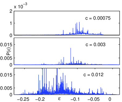
Figure 6: (color online) Inverse participation ratio for $V_{L}=8t$ and different impurity concentrations.

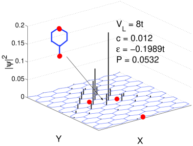
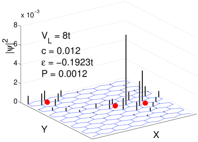
Figure 7: (color online) Fragments of eigenstates for $V_{L}=8t$ and $c=0.012$ are depicted. These configurations of impurities are characteristic for the second peak in the DOS.

In addition, to study the character of states within this domain, we calculated the inverse participation ratioPereira $P(\varepsilon)$ as a localization criterion in a system of a smaller size:

$$P(\varepsilon)=\sum\limits_{\bm{n}_{\alpha}}|\psi_{\bm{n}_{\alpha}}|^{4},$$ (11)

where summation runs over all lattice sites. Even though the comparison for systems of different size is not included in the current article, we should mention that the hight of $P(\varepsilon)$ curves does not diminish with increasing the size of the system suggesting electron localization. The dynamics of the inverse participation ratio with increasing the impurity concentration is given in Fig. 6. Here again periodical boundary conditions were used at zigzag edges of the sample to get rid of the sharp peak at $\varepsilon=0$, which is related to boundary states. Chosen concentrations repeat those from Fig. 4 that corresponds to the same impurity potential. A radical localization intensification after the spectrum rearrangement is evidently seen. States are showing a tendency for their localization in the very region, in which the CPA is not valid. This fact also confirms a close connection between the CPA applicability criterion and the Ioffe-Regel criterion.Ioffe When comparing Fig. 6 to Fig. 4, in particular at $c=0.012$, it is obvious that the largest values of $P(\varepsilon)$ match the peaks in the DOS.

A pair of states corresponding to the sharp peaks in the inverse participation ratio graph are shown in Figs. 7 and 8. The states corresponding to the first (counting from $\varepsilon=0$) maximum in the DOS at $\varepsilon\approx-0.14t$ are mostly represented by relatively distant impurity pairs and triads. Equally challenging is the origin of the second DOS peak at $\varepsilon\approx-0.19t$. The visualization of the wave-function belonging to this region is provided in Fig. 7. It shows that this peak is largely due to the characteristic pattern of impurities, which is depicted in the same figure. It is worth mentioning that impurity atoms are located on one sublattice for these strongly localized states, while the $\psi$-function is concentrated on the other sublattice. It resembles the situation with a double impurityKatsnelson and can be attributed to the relation $|g_{\bm{0}_{\alpha}\bm{n}_{\alpha}}|\ll|g_{\bm{0}_{\alpha}\bm{n}_{\beta}}|$ for $|\varepsilon|\rightarrow 0$. To summarize, when the critical concentration of impurities is exceeded, a quasigap filled with localized states is developing in the graphene’s spectrum because of the impurity cluster effects. Since the CPA does not account for cluster effects and scatterings by impurity clusters dominate within this quasigap, the CPA is not applicable in this region.

Numerical results show that Dirac point as such is eliminated from the spectrum when the critical concentration $c_{r}$ is reached. Consequently, it is not justifiable to speak about the Dirac point existence, albeit the impurity concentration can be relatively low (as low as $c_{r}$ is). The CPA and the ATA do not correctly describe the DOS minimum between the valence band and the conduction band for $c>c_{r}$. Normally, the Dirac point coincides with the Fermi energy for the pure (or undoped) graphene. However, at the finite concentration of impurities situation changes drastically. Dean’s approach allows to track the position of the Fermi level, since it outputs the total number of states located below any given energy. The Fermi level monitoring revealed that its position shifts in the positive direction away from the DOS minimum. The greater is the impurity concentration the more prominent is the Fermi energy shift from the DOS minimum, which transforms graphene into a “doped” conductor without any gate voltage applied. Should impurity atoms bring additional electrons in the system, the doping effect will be increased.

This shift can be explained by the following uncomplicated consideration. Without the conduction band, the valence band should develop a strong tail above its upper edge for a positive impurity potential $V_{L}>0$. Since the conduction band is not separated from the valence band, this tail falls inside the conduction band producing excessive states above the DOS minimum. Keeping in mind that total number of states within the single band should be preserved because of the sum rules, this expansion of the valence band into the conduction band yields a deficit of states below the DOS minimum. At the constant amount of carriers, extra electrons are flowing out to the conduction band altering the Fermi level position. With increasing impurity concentration the tail is gradually becoming more pronounced, which consequently makes the shift in the Fermi energy more apparent.

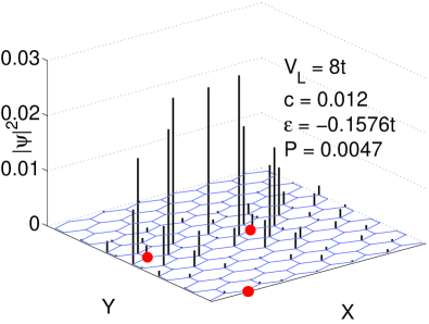
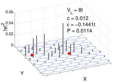
Figure 8: (color online) Fragments of the eigenstates for $V_{L}=8t$ and $c=0.012$ are depicted. They correspond to the first (closest to the Dirac point) peak in the DOS.

IV Conclusion

A comprehensive analysis of the spectrum rearrangement in graphene with substitutional impurities by numerical simulation has been carried out. We studied the DOS near the Fermi level in graphene for a set of impurity potentials and impurity concentrations.

It was demonstrated that indeed a certain characteristic concentration of impurities can be specified, at which the graphene’s spectrum undergoes a qualitative change. This critical impurity concentration is associated with the spatial overlap of individual impurity states. In a turn, it has been established that the cardinal modification of the spectrum is manifested by the opening of the filled with highly localized states quasigap around the impurity resonance energy. The cluster effects were found to be responsible for the quasigap formation. Pair impurity states representing the most prominent peaks in the DOS within the quasigap have been visualized, which emphasized the dominance of scatterings on impurity clusters inside the quasigap. Aforesaid confirmed the predicted scenario of the spectrum rearrangement in graphene.

A comparison of the CPA DOS with the numerically simulated DOS supported the suggested CPA applicability criterion and its efficacy as an instrument in the description of the spectrum rearrangement passage. As well, intimate correlation between the CPA validity and the degree of electron localization has been revealed. That is, inside the quasigap, in which cluster effects are essential and states are localized, the CPA is not reliable.

Furthermore, we report about the phenomenon of the Fermi level shift from the DOS minimum — a kind of a self-doping, which alters the conductivity of impure graphene without gate voltage variation even in the case of neutral impurities.

- (1) K. S. Novoselov, A. K. Geim, S. V. Morozov, D. Jiang, Y. Zhang, S. V. Dubonos, I. V. Grigorieva, and A. A. Firsov, Science 306, 666 (2004).
- (2) F. Schedin, A. K. Geim, S. V. Morozov, D. Jiang, E. H. Hill, P. Blake, and K. S. Novoselov, Nat. Mater. 6, 652 (2007).
- (3) T. O. Wehling, A. V. Balatsky, M. I. Katsnelson, A. I. Lichtenstein, K. Scharnberg, and R. Wiesendanger, Phys. Rev. B 75, 125425 (2007).
- (4) V. M. Pereira, F. Guinea, J. M. B. Lopes dos Santos, N. M. R. Peres, and A. H. Castro Neto, Phys. Rev. Lett. 96, 036801 (2006).
- (5) N. M. R. Peres, F. Guinea, and A. H. Castro Neto, Phys. Rev. B 73, 125411 (2006).
- (6) Ben Yu-Kuang Hu, E. H. Hwang, and S. Das Sarma, Phys. Rev. B 78, 165411 (2008).
- (7) V. M. Pereira, J. M. B. Lopes dos Santos, and A. H. Castro Neto, Phys. Rev. B 77, 115109 (2008).
- (8) S. Wu, L. Jing, Q. Li, Q. W. Shi, J. Chen, X. Wang, and J. Yang, Phys. Rev. B 77, 195411 (2008).
- (9) Yu. V. Skrypnyk and V. M. Loktev, Phys. Rev. B 73, 241402(R) (2006).
- (10) Yu. V. Skrypnyk and V. M. Loktev, Low Temp. Phys. 33, 762 (2007).
- (11) Yu. V. Skrypnyk, Phys. Rev. B 70, 212201 (2004).
- (12) M. A. Ivanov, V. M. Loktev and Yu. G. Pogorelov, Phys. Rep. 153, 209 (1987).
- (13) P. Dean, Rev. Mod. Phys. 44, 127 (1972).
- (14) A. Bostwick, T. Ohta, T. Seyller, K. Horn and E. Rotenberg, Nature Physics 3, 36 (2007).
- (15) R. J. Elliot, J. A. Krumhansl, and P. L. Leath, Rev. Mod. Phys., 46, 465 (1974).
- (16) I. M. Lifshits, S. A. Gredeskul, and L. A. Pastur, Introduction to the Theory of Disordered Systems, Wiley, N.Y. (1988).
- (17) C. Bena, Phys. Rev. B 79, 125427 (2009).
- (18) R. Haydock, V. Heine, and M. J. Kelly, J. Phys. C 5, 2845 (1972).
- (19) A. R. Akhmerov and C. W. J. Beenakker, Phys. Rev. B 77, 085423 (2008).
- (20) A. F. Ioffe and A. R. Regel, Prog. Semicond. 4, 237 (1960).