Fast Surface Based Electrostatics for biomolecules modeling.

Abstract

We analyze deficiencies of commonly used Coulomb approximations in Generalized Born solvation energy calculation models and report a development of a new fast surface-based method (FSBE) for numerical calculations of the solvation energy of biomolecules with charged groups. The procedure is only a few percents wrong for molecular configurations of arbitrary sizes, provides explicit values for the reaction field potential at any point of the molecular interior, water polarization at the surface of the molecule, both the solvation energy value and its derivatives suitable for Molecular Dynamics (MD) simulations. The method works well both for large and small molecules and thus gives stable energy differences for quantities such as solvation energies contributions to a molecular complex formation.

I Introduction.

Solvent plays an essential role in biophysics in determining the electrostatic potential energy of proteins, small molecules and protein-ligand complexes. Solvation energy is a major contribution to the protein folding problem and to ligand binding energy calculations. In the latter case it is the interaction, which is pretty much responsible for binding selectivity (Schaefer and Karplus, 1996; Gilson and Zhou, 2007). Large scale Molecular Dynamics (MD) simulations (Allen and Tildesley, 1989; Janežič et al., 2005; Praprotnik and Janežič, 2005) or industrial-scale calculations of the solvation energy in drug discovery applications require a fast method capable of dealing with arbitrary molecular geometries of molecules of vastly different sizes within a single, fast, numerically robust framework.

A solvation energy calculation for a molecule-sized object has always been and still is a challenging problem. The most accurate approach is, apparently, a large scale MD simulation (Rapaport, 2004b, a) of the body of interest immersed in a tank of water molecules in a realistic force field or even within quantum mechanical settings. Although being ideologically correct such calculations are time consuming and pose a number of specific problems stemming, e.g. from long relaxation times of water clusters. One possible way to bridge such “simulation gap” is to employ different types of continuous solvation models. Fortunately, water is characterized by a very large value of dielectric constant and therefore to a large extent the reaction field of water molecules has a collective nature. Although realistic properties of molecular interactions depend both on short-scale water molecules alignment and on their long-range dipole-dipole interactions at the same time (Fedichev and Menshikov, 2008, 2006), purely electrostatic models, such as Poisson-Boltzmann equation solvers (Baker et al., 2001; Schäfer et al., 2000), turned out to be very successful in various applications.

Even within the realm of continuous electrostatic models there are numerous approaches in use to calculate the electrostatic contribution to solvation energies. Popular techniques span from finite element methods (FEM, (Baker et al., 2001; Schäfer et al., 2000; Bordner and Huber, 2003; Boschitsch et al., 2002; Boschitsch and Fenley, 2004; Horvath et al., 1996; Vorobjev and Scheraga, 1997; Zhou, 1993)) to multiple variations of Generalized Born (GB) approximations (Schaefer and Karplus, 1996; Still et al., 1990; Tsui and Case, 2001; Simonson, 2001; Lee et al., 2002; Hassan and Mehler, 2002; Rashin, 1990; Feig et al., 2004; Onufriev et al., 2002). A numerical FEM solution to the Poisson-Boltzmann equation (PBE) is a formally fast (the calculation time and memory scale $\propto N,$ with $N$ being the number of particles in the system) and is a rigorous attempt to solve the electrostatics problem. On the other hand GB approximations are practically fast, in spite of the fact that it normally takes $O(N^{2})$ operations to calculate GB energy. Unfortunately GB approximations are very rough and that is why GB calculations work well only for small and medium sized molecules, whereas FEM methods can, although at expense of numerical complexity, be applied to very large systems. The particular boundary between the applicability of the two methods is vague and depends, in terms of speed, on the details of the methods realization, and, in terms of accuracy, on the system geometry (see below).

In this Paper we report a development of a new fast surface-based method (FSBE) for numerical calculations of the solvation energy of biomolecules with charged groups. First we elucidate physical nature of commonly used GB models, identify the variational principle behind and discharge the so called Coulomb approximation. As a result we suggest a new computational procedure, which is only a few percents wrong for any molecular configurations of arbitrary sizes, gives explicit values for the reaction field potential at any point inside a molecule, characterizes the water polarization charge density on the molecule interfaces. The approach reported here is suitable both for the solvation energy and its derivatives calculation for Molecular Dynamics (MD) simulations. The method works well both for large and small molecules and thus gives stable energy differences for quantities such as solvation energies of molecular complexes formation.

An important side effect of our studies is a comparative research of various GB approximations. We distinguish between the volume and surface based approaches to calculate the Born radii of the charges and demonstrate that only the latter can be trusted. The reason is that any practical way of volume overlaps integrals calculation implies some sort of weak atomic overlap approximation and hence effectively leaves many unphysically small water-filled cavities within the molecules. This leads to an overestimation of both the molecular volume and the dielectric constant of the molecular interior. Both factors essentially disrupt accurate descreening calculations and often lead to completely unrealistic results.

The manuscript is organized as follows. Section II provides an overview of continuous solvation energy calculation methods. We compare exact Poisson-Boltzmann equation solvers to approximate GB models and highlight deficiencies of commonly used Coulomb approximations. In the subsequent Section III we represent the idea of a new fast molecular surface based method and estimate its accuracy for a number of exactly solvable cases. In Section IV we discuss important numerical implementation details and, at last, in Section V, we demonstrate performance of the method in realistic modeling examples. At the end of the presentation we hint how explicit expressions for the surface charge densities and the reaction field potential may help building $O(N)$ methods for approximate solvation energies calculations (Fedichev et al., 2009).

II Overview of existing methods.

To elucidate the nature of approximations and limitations of GB family of approaches it is instructive to start from the basics physics. To find the polar contribution to the solvation energy in a continuous solvation model, $E_{S}$, one should solve the Poisson equation

$$\triangle\varphi(\mathbf{r})=-4\pi\rho(\mathbf{r})$$ (1)

for the potential $\varphi(\mathbf{r})$ generated by the charge density

$$\rho(\mathbf{r})=\sum_{i}q_{i}\delta\left(\mathbf{r-\mathbf{r}}_{i}\right),$$ (2)

defined by the atoms placed at the positions $\mathbf{\mathbf{r}}_{i}$, and the boundary conditions at the molecules surfaces and spatial infinity.

There are various ways to calculate the potential $\varphi(\mathbf{r})$. The most practical approach is to use some sort of finite elements method (FEM), which can be both in volume and boundary grids incarnations (see e.g. (Rashin, 1990; Zhou, 1993; Zauhar, 1995; Horvath et al., 1996; Vorobjev and Scheraga, 1997; Bordner and Huber, 2003; Boschitsch et al., 2002; Boschitsch and Fenley, 2004; Schäfer et al., 2000)). The boundary grid based methods are often more practical and aside from subtle details are equivalent to Surface Electrostatic Solvation (SES) models. A typical SES-water model can be considered as an alternative to discretization of the volume and is given by the solution of the following integral equation

$$2\pi\sigma_{j}\left(\mathbf{r}\right)+\int_{\Gamma_{W}}df^{\prime}\sigma_{j}\left(\mathbf{r}^{\prime}\right)\frac{\mathbf{n\left(\mathbf{r}-\mathbf{r}^{\prime}\right)}}{\left|\mathbf{r}-\mathbf{r}^{\prime}\right|^{3}}=-q_{j}\frac{\mathbf{n}\left(\mathbf{r}-\mathbf{r}_{j}\right)}{\left|\mathbf{r}-\mathbf{r}_{j}\right|^{3}}$$ (3)

for the polarization charges surface density $\sigma_{j}\left(\mathbf{r}\right)$ at the point $\mathbf{r}$ on the molecule’s surface induced by the protein charges $q_{j}$ as shown on Fig. 1. Here $df^{\prime}$ is the element of the molecular surface at a point $\mathbf{r}^{\prime}$, $\mathbf{n}$ is the unit normal to the surface at the point $\mathbf{r}$. The exact formula for solvation energy is then:

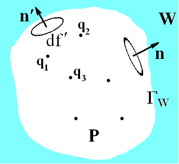
Figure 1: Solvation energy calculation problem setup: schematic representation of a macromolecule (see the explanations in the text).

$$\left(E_{S}\right)_{ex}=\frac{1}{2}\sum_{i}q_{i}\varphi_{1}(\mathbf{r}_{i}),$$ (4)

where

$$\varphi_{1}(\mathbf{r})=\sum_{j}\int_{\Gamma_{W}}df^{\prime}\frac{\sigma_{j}\left(\mathbf{r}^{\prime}\right)}{\left|\mathbf{r}-\mathbf{r}^{\prime}\right|}$$ (5)

stands for the so called reaction field potential, produced by the water polarization charges on the boundary of the molecule $\Gamma_{W}$. The total electric potential consists of the two parts:

$$\varphi(\mathbf{r})=\varphi_{0}(\mathbf{r})+\varphi_{1}(\mathbf{r}),$$ (6)

where

$$\varphi_{0}(\mathbf{r})=\sum_{j=1}^{N}\frac{q_{j}}{\left|\mathbf{r}-\mathbf{r}_{j}\right|}$$ (7)

is the potential of the charges in vacuum, i.e. in the absence of the water molecules. Since water is characterized by a large value of the dielectric constant,$\epsilon_{W}\approx 80\gg 1$, to a good accuracy the electric potential vanishes inside the water bulk so that

$$\varphi(\mathbf{r})\mid_{\Gamma_{W}}=0$$ (8)

on the boundaries. The model implies that the dielectric constant of the liquid is infinitely large, whereas the dielectric constant of the molecules interior is $1$. Although the method is fairly easy to implement, it is also not very practical: in realistic applications involving large molecules the calculation is memory consuming, slow and not very stable with respect to small changes in the surface elements positions and orientations. The latter circumstance also means that both FEM and SES methods often fail to provide smooth derivatives of the solvation energies suitable for MD studies of bio-molecules.

A very well known alternative to solving the Poisson-Boltzmann equation directly is to use generalized Born (GB) approximation, which is a fast, simple, qualitatively correct and numerically stable method for macromolecular solvation effects calculations (Still et al., 1990; Tsui and Case, 2001; Lee et al., 2002; Bashford and Case, 2000; Onufriev et al., 2002). The method is based on the following ad hoc. approximate expression for the full electrostatic energy $E_{el}$ for system of charges charges $q_{i}$ located within the surface $\Gamma_{W}$ separating the molecule from the water environment:

$$E_{el}=\frac{1}{2}\sum_{i\neq j}\frac{q_{i}q_{j}}{\epsilon_{P}r_{ij}}+\left(E_{S}\right)_{GB}.$$ (9)

The notations used in the expression are illustrated on Fig.1. Here the indices $i,j=1,...,N$ enumerate the charges, $N$ is the number of charges, $\mathbf{r}_{ij}=\mathbf{r}_{i}-\mathbf{r}_{j}$, $r_{ij}=\left|\mathbf{r}_{ij}\right|$, $\mathbf{r}_{i}$ is the radius-vector of a charge $i$ ($i$-th atom),

$$\left(E_{S}\right)_{GB}=-\frac{1}{2}\sum_{i,\,j}\frac{q_{i}q_{j}}{f_{GB}\left(r_{ij}\right)}\left(\frac{1}{\epsilon_{P}}-\frac{1}{\epsilon_{W}}\right),$$ (10)

$\epsilon_{P}$ and $\epsilon_{W}$ are dielectric constants for within the molecule interiors and water, correspondingly. The factor $f_{GB}\left(r_{ij}\right)$ is commonly (although not always) defined as

$$f_{GB}\left(r_{ij}\right)=\left[r_{ij}^{2}+R_{Bi}R_{Bj}exp\left(-r_{ij}^{2}/4R_{Bi}R_{Bj}\right)\right]^{1/2}.$$ (11)

The effective Born radii $R_{Bi}$ of the ions are calculated according to

$$\frac{1}{R_{Bi}}=\frac{1}{4\pi}\int_{W}\frac{1}{s_{i}^{4}}d^{3}r^{\prime}=\frac{1}{4\pi}\int_{\Gamma_{W}}\frac{\left(\mathbf{n^{\prime}}\mathbf{s}_{i}\right)}{s_{i}^{4}}df^{\prime},$$ (12)

where $s_{i}=\left|\mathbf{s}_{i}\right|$, $\mathbf{s}_{i}=\mathbf{r}^{\prime}-\mathbf{r}_{i}$. In its volume integral representation Eq. (12) assumes the integration over the water bulk $W$, which can be easily transformed to an equivalent boundary integral form in a standard way with the help of the Gauss theorem (Ghosh et al., 1998).

Various models are used to define molecular surfaces and volumes. Normally the molecule volume is approximated as a set of spheres of specified radii $a_{i}$, the individual ions Born radii, centered at the points of the charges locations and thus characterizing water cavities associated with the ions in the solute. Therefore a complete GB model should also include a set of fitting parameters $a_{i}$. The specific values of the model radii $a_{i}$ are either set to the atomic van der Waals radii, or (better) trained to reproduce experimental values of the polar part of small molecules solvation energies whenever it is possible. In spite of being only a very rough approximation, GB models are widely used in practical simulations.

Common deficiencies of GB approximation are very well known. Consider, e.g., a single charge $q$ fixed at a distance $r$ from the center of a spherical molecule of a radius $a$. Eqs. (10)-(12) immediately yield:

$$\frac{1}{R_{B}}=\frac{1}{4r}\log\left(\frac{a+r}{a-r}\right)+\frac{a}{2\left(a^{2}-r^{2}\right)},$$ (13)

$$\left(E_{S}\right)_{GB}=-\frac{q^{2}}{2R_{B}}$$ (14)

On the other hand the problem is simple and can be solved exactly both for the reaction field potential (Stratton, 1941; Jackson and Fox, 1999):

$$\varphi_{1}(\mathbf{r})=-\sum_{j}\frac{q_{j}}{\left|\frac{r_{j}\mathbf{r}}{a}-a\widehat{\mathbf{r}}_{j}\right|},$$ (15)

($\hat{\mathbf{r}}_{j}=\mathbf{r}_{j}/r_{j}$), and the solvation energy

$$\left(E_{S}\right)_{ex}=-\frac{1}{2}\sum_{i,j}\frac{q_{i}q_{j}}{\sqrt{\left(\frac{r_{i}r_{j}}{a}\right)^{2}+a^{2}-2\mathbf{r}_{i}\mathbf{r}_{j}}}$$ (16)

for an arbitrary number of the charges within the sphere. The solution has been long advocated by Kirkwood (Kirkwood, 1934; Tanford and Kirkwood, 1957)and takes especially simple form for a single charge

$$\left(E_{S}\right)_{ex}=-\frac{q^{2}a}{2\left(a^{2}-r^{2}\right)}.$$ (17)

The approximate GB solution (14) fails to reproduce the exact result (17) for the solvation energy of an ion within a spherical cavity, as shown on Fig.2. The solvation energy and hence the Born radius are in a good agreement with the exact result if the charge is close to the cavity center and are off by a factor of $2$ if the charge is next to the molecular surface. Realistic biomacromolecules are large and most of their charges are close to molecular surfaces. In the very same time the GB approximation in its most commonly accepted form fails exactly next to the molecular surface. This means that there is no way to “train” the seed values of the Born radii to reproduce the solvation energies of both small and large molecules. This also means that GB models in the standard form can not predict well solvation energy contributions to ligand binding free energies in drug discovery applications. Indeed, drug binding affinity depends on the solvation energy difference between a protein-ligand complex and the protein-ligand pair separated at infinity. The proteins are large and ligands are normally small molecules with all the substantial charges of the protein-ligand complex arranged close to the (large) protein surface.

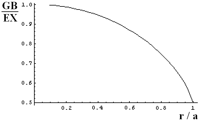
Figure 2: Ratio of GB solvation energy to exact one for the model spherical “protein” of a radius $a$ as a function of the charge position $r$ from the center of the sphere.

The reason why GB approaches fail becomes clear from comparison with the exact expression

$$\left(E_{S}\right)_{ex}=\left(E_{S}\right)_{GB}+\triangle E_{S}<\left(E_{S}\right)_{GB},$$ (18)

where

$$\triangle E_{S}=-\int_{P}dV\frac{1}{8\pi}\left(\nabla\varphi_{1}\right)^{2}<0,$$

where the integration is performed over the molecule interior $P$. GB approximation accounts for the electrostatic energy of the polarization charges (reaction field) incorrectly and, in fact, overestimates it. Eq. (18) suggests that GB is nothing else but a variational calculation of the solvation energy. The “probe function” (10) is widely tested and trusted, whereas specific recipes for the Born radii calculations can still be different. The popular choice, Eq. (12), corresponds to the so called Coulomb approximation (CA, see (Bashford and Case, 2000) and the refs. therein for a review). CA does not follow from any first principles and puts severe limitation on applications of GB models. Up to date there have been a few sound attempts to go beyond CA and obtain better recipes for the Born radii as discussed, e.g., in (Ghosh et al., 1998; Romanov et al., 2004). In what follows we dwell into the physics behind the Born radii calculations and generate a whole family of approximations for molecular electrostatics.

III How to find Born radii?

In this section we part from CA and demonstrate a new way to calculate the polar part of the solvation energy. The practical goal is to combine the accuracy of FEM or SES models with the speed and numerical stability of GB approximation. To prove this is possible we identify GB solution as a possible variational solution of the Poisson equation (1). Given a set of known positions of the atom charges, we suggest the following GB-like anzatz for the reaction field potential $\varphi_{1}$:

$$\varphi_{1}(\mathbf{r})=-\sum_{j}\frac{q_{j}}{\sqrt{\left(\mathbf{r}-\mathbf{r}_{j}\right)^{2}+R\left(\mathbf{r}\right)R_{j}}},$$ (19)

where$R\left(\mathbf{r}\right)$ is the variational function, $R_{j}\equiv R(\mathbf{r}_{j})$. The true solution of the electrostatics problem provides the minimum to the functional:

$$G_{2}[R(\mathbf{r})]=\int_{P}dV\frac{1}{8\pi}\left(\nabla\varphi_{1}\right)^{2}.$$

Since the potential vanishes at the molecule boundary Eq. (8) suggests a very simple boundary condition for the variational function $R\left(\mathbf{r}\right)$: $R\left(\mathbf{r}\right)|_{\Gamma_{W}}=0$.

The potential in the form of Eq. (19) is an approximation already. The best possible function $R\left(\mathbf{r}\right)$ should provide the minimum to the functional $G_{2}$. To find such a solution may be an interesting problem in itself. Nevertheless it is not practically: optimization of the functional $G_{2}$ is roughly as easy (or difficult) as to find the exact solution of the Poisson equation. To avoid this unnecessary procedure of the functional minimization we suggest instead a specific form of the function $R\left(\mathbf{r}\right)$

$$\frac{1}{\left[R\left(\mathbf{r}\right)\right]^{3}}=\frac{3}{4\pi}\int_{W}\frac{1}{\left|\mathbf{r^{\prime}}-\mathbf{r}\right|^{6}}d^{3}r^{\prime},$$ (20)

in the “classic” volume integration form, or, equivalently, in the surface integration form

$$\frac{1}{R_{i}^{3}}=\frac{1}{4\pi}\int_{\Gamma_{W}}\frac{\left(\mathbf{n^{\prime}}\mathbf{s}_{i}\right)}{s_{i}^{6}}df^{\prime},$$ (21)

for each of the charges. Here $s_{i}=\left|\mathbf{s}_{i}\right|$, $\mathbf{s}_{i}=\mathbf{r}^{\prime}-\mathbf{r}_{i}$, and the polar part of the solvation energy (the reaction field energy) is given by a Kirkwood like expression

$$\left(E_{S}\right)_{FSBE}=-\frac{1}{2}\sum_{i,j}\frac{q_{i}q_{j}}{f_{ij}}$$ (22)

with $f_{ij}=f(\mathbf{r}_{i},\mathbf{r}_{j})=\sqrt{r_{ij}^{2}+R\left(\mathbf{r}_{i}\right)R\left(\mathbf{r}_{j}\right)}=\sqrt{r_{ij}^{2}+R_{i}R_{j}}$.

Although at a first glance FSBE approach does not seem to be very different from GB approximation, the solution (19) is a much better approximation to the solution of the original electrostatic problem. To see that let us turn back to the example of a charge confined within a spherical cavity of radius $a$. The new improved Eq. (20) for the “generalized” Born radius gives

$$R\left(\mathbf{r}\right)=\left(a^{2}-r^{2}\right)/a,$$ (23)

which, after inserting into Eq. (19) gives the exact results for the reaction field potential (15) and the solvation energy of the point charge (16) within the sphere. It can be further shown that FSBE approach is exact for arbitrary configuration of charges confined within a spherical cavity of arbitrary size. This means FBSE is exact both for ions next to a large protein boundary and in a center of a small sphere representing a single ion. The FSBE gives also the exact result for arbitrary configuration of multiple charges next to the spherical water cavern inside a large protein.

Our direct interpretation of the reaction field potential helps us to find the polarization surface charge density $\sigma_{S}$ at the interface boundary. Indeed, the standard form of the electrostatics boundary condition for the electrostatic potential reads:

$$\sigma_{S}=\frac{1}{4\pi}\frac{\partial\varphi}{\partial n},$$

where

$$\varphi(\mathbf{r}^{\prime})=\varphi_{0}+\varphi_{1}=\sum_{j}q_{j}\left(\frac{1}{\left|\mathbf{r}^{\prime}-\mathbf{r}_{j}\right|}-\frac{1}{f(\mathbf{r}^{\prime},\mathbf{r}_{j})}\right)$$

is the full electrostatic potential. Next to the boundary ($\mathbf{r}^{\prime}\rightarrow\Gamma_{W}$) $R\left(\mathbf{r}^{\prime}\right)\approx 2h\rightarrow 0$, where $h$ is the distance from a given point to the surface. Combining the expressions above we obtain:

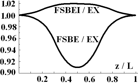
Figure 3: Ratio of FSBE solvation energy to exact value for one charge inside protein in the form of a layer with thickness $L$ (the lower curve). The upper curve describe the result of the improved approach FSBEi (see below).

$$\sigma_{S}(\mathbf{r}^{\prime})=-\frac{1}{4\pi}\sum_{j}q_{j}\frac{R_{j}}{\left|\mathbf{r}^{\prime}-\mathbf{r}_{j}\right|^{3}}.$$ (24)

Note, that the standard GB approach may, in principle, also be used to calculate $\sigma_{S}$. Nevertheless such an approximation would not be good since GB approximation for $R\left(\mathbf{r}\right)$ is twice as small than that of the exact result (23).

FSBE can not, of course, be exact for an arbitrary molecule geometry. Eqs. (20) and (22) are certainly only approximate. To see the limitations of the approach we explored various exactly solvable charges configurations. Consider the first example: a plain layer-like “molecule” (or membrane) of the thickness $L$ surrounded by the continuous water on both sides with a charge $q$ placed inside the layer at the distance $z$ from one of the water interface planes. The exact result for solvation energy is (Stratton, 1941; Jackson and Fox, 1999)

$$\left(E_{S}\right)_{ex}=q^{2}\int_{0}^{\infty}dk\left[\frac{\sinh\left(kz\right)\sinh\left(k\left(L-z\right)\right)}{\sinh\left(kL\right)}-\frac{1}{2}\right].$$ (25)

Eqs. (20) and (22) be used to find FSBE approximation for the solvation energy

$$\left(E_{S}\right)_{FSBE}=-q^{2}\frac{\sqrt[3]{1-3\overline{z}\left(1-\overline{z}\right)}}{4z\left(1-\overline{z}\right)},$$

where $\bar{z}=z/L$. Once again, to characterize the difference between the approximate FSBE and the exact results we plotted the ratio of $\left(E_{S}\right)_{FSBE}$ to the exact solvation energy $\left(E_{S}\right)_{ex}$ on Fig.3. As in our spherical cavity example above the two results coincide at the dielectric boundary (as it should be) and deviate from each other in the center of the layer. The discrepancy does not exceed $9\%$, which is nothing compared with the factor of $2$ in the case of the standard GB approximation.

Another challenging case is the calculation for a single charge $q$ placed within a corner made of two perpendicular infinite walls (the “$xz$” and “$yz$” planes). Once again, our FSBE result

$$\left(E_{S}\right)_{FSBE}=-q^{2}\frac{\sqrt[3]{1-\frac{3}{2}\left(\sin\varphi\cos\varphi\right)^{2}}}{4r\sin\varphi\cos\varphi},$$

where $\varphi$ is the azimuthal angle between the position of a charge and the “xz” plane, $r$ is the distance from the charge and “z” axes (the intersection of the walls). The result should be compared with the exact solvation energy

Figure 4: Ratio of FSBE solvation energy to exact value for one charge inside the corner between two perpendicular infinite walls (the lower curve). The upper curve describes the result of the improved approach FSBEI (see below).

$$\left(E_{S}\right)_{ex}=-q^{2}\frac{\sin\varphi+\cos\varphi-\sin\varphi\cos\varphi}{4r\sin\varphi\cos\varphi}.$$

Once again, the ratio of the two energies is plotted on Fig.4. The difference is no more than $6\%$ in the center of the system and disappears at the corner boundaries (as it should be).

The presented results prove that Eqs.(20) and (22) defining FSBE approximation do provide a fairly good solution of the electrostatic problem in various geometries. Whenever a charge is placed close to an interface boundary, FSBE becomes exact; for charges placed at the central regions of a large molecule the error is about $10\%$, which is fair and often not very important, since most of the charges in biomolecules are located in a layer next to molecular surfaces. This error can be lowered up to $2\%$ by further variational improvements of FSBE (see below).

Before we proceed to explicit description of the method implementation, let us take a note on volume and surface integrals methods for Born radii calculations. Practical applications of Generalized Born models are further complicated by various approximations introduced for volume (or surface) integrals calculations. Since direct calculations are often prohibitively time consuming, the integrals are often estimated in various sort of pair approximations with subsequent removal of the atom overlaps etc. Obviously atoms in biomolecules are fairly densely packed and the approximation lead to wrong molecular volumes and very wrong (even negative(!)) values for the Born Radii for every atom.

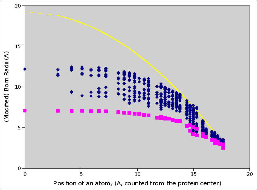
Figure 5: Born radii calculated for an ion placed at different positions inside a model “protein” made of $1000$ carbon atoms.

Physically speaking Born radii quantitatively show a degree to which an atom is "buried" within a molecule, such as a protein. Fig.5 gives a simple idea to which extent GB can even be used for description of solvation energies of a simple, model spherical “protein” molecule built of approx. $1000$ carbon atoms. The red squares represent Born Radii as a function of an ion position off the center of the “protein”. The values were obtained using our own implementation of AGBNP method (Gallicchio and Levy, 2004), one of the best realizations of GB procedures available in the literature. The yellow curve represents exact result for a spherical protein. As one can see, AGBNP results fail grow enough inwards and saturates at a very small value at the “protein” center.

The explanation is the following: AGBNP (and for that reason practically any other GB model based on volume integrals approximations) implies a certain implicit approximation for the shape of molecular surface. Since the model equations employed for the atomic overlap integrals do not provide a direct interpretation, it turns out that the overlap integrals are often not exact. Physically this means that there are effectively numerous water filled cavities of nonphysically small sizes assumed inside the protein. The cavities are so small that can not hold a single water molecule inside, though represent (within the same model) a medium with high dielectric constant, effectively increase the dielectric constant of the “protein” and therefore decrease the value of the Born radii. To check the hypotheses we implemented a simple algorithm to search for the water filled cavities and remove them (to a certain adjustable extent). The result is represented by the blue circles and shows a clear improvement towards reproducing the exact analytical result. The simple exercise shows that volume integral based Born models overestimate the dielectric constant within the molecule and may easily lead to a number of undesired unphysical issues. In practice any approach based on a calculation of surface integrals for Born radii has much better chances to yield meaningful results.

Fig.5 demonstrates another feature of Born approximations. As discussed earlier CA fails at the protein boundary and gives the Born radius which is twice the exact result (see the dots on the right compared to the yellow line). This is a genuine problem of CA and can be solved by, e.g. switching to FSBE expressions for Born radii.

In principle, Eq. (20) can be used to calculate Born radii directly. Unfortunately such a procedure is too slow for realistic molecules with typical number of atoms $N\sim 10^{4}$. Below we will show that FSBE in the form of Eq. (21) yields to a much better GB solvation energy calculation implementation. Since the solvation energy is often used in MD simulations, we need also analytical and easily implementable prescriptions for the forces calculations, i.e. energy derivatives with respect to the atomic positions:

$$\frac{\partial E_{S}}{\partial\mathbf{r}_{j}}=q_{j}\sum_{k}\frac{q_{k}\mathbf{r}_{jk}}{\left(f_{jk}\right)^{3}}+\frac{1}{2}\sum_{i,k}\frac{q_{i}q_{k}}{\left(f_{jk}\right)^{3}}R_{k}\frac{\partial R_{i}}{\partial\mathbf{r}_{j}}.$$ (26)

Let us show how our surface integral representation of the Born radii (21) let us to express the forces in terms of the surface integrals. To calculate the derivative $\partial R_{i}/\partial\mathbf{r}_{j}$ we shift the atom $j$ with coordinates $\mathbf{r}_{j}$ by a small value $d\mathbf{r}_{j}$ and observe how the surface elements $d\mathbf{f^{\prime}}$ are affected by the atom move. Then the molecule volume changes by the value $dV=d\mathbf{r}_{j}d\mathbf{f^{\prime}}$, which lets us calculate the Born radius change using the Eq.(21) as follows

$$\frac{\partial R_{i}}{\partial\mathbf{r}_{j}}=\frac{R_{i}^{4}}{4\pi}\int_{\Gamma_{W}^{j}}\frac{\mathbf{n^{\prime}}}{s_{i}^{6}}df^{\prime},\quad j\neq i,$$ (27)

$$\frac{\partial R_{i}}{\partial\mathbf{r}_{i}}=-\sum_{j\neq i}\frac{\partial R_{i}}{\partial\mathbf{r}_{j}},$$ (28)

where $\Gamma_{W}^{j}$ represents the part of the molecular surface influenced by the atom $j$. In the following section we show how GB implementation defined by Eqs. (21), (26) and (27) performs in a few model and realistic situations.

IV Results and discussion.

FSBE is not mere another method for quantitatively correct molecular modeling calculations. In what follows shortly we will show that FSBE calculations have a number of important properties besides its speed. To see that let us consider a few model calculations to show the method performance in a number of simple but challenging limiting cases.

A diatomic molecule is the simplest but the at the same time conceptually important example of a realistic solvation energy calculation. The trick is that any reasonable solvation energy model gives exact value for a single atom. Depending on the radii of and the distances between the atoms the solvation energy of a pair may be a very good test of a solvation energy model and transferability of its parameters.

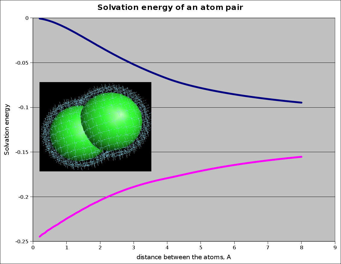
Figure 6: Solvation energy of a diatomic molecule (in units of $1389\,kJ\cdot\text{\AA}/(mol\cdot e^{2})$) in frames of FSBE approach. The green spheres at the inset represent ions, the blue crosses represent the surface points that were used in calculation.

Fig.6 shows the FSBE calculated solvation energies for a pair of model ions with similar (red curve) and opposite (blue) charges of $1/2$ atomic units each. The results are pleasing and easy to understand. At infinite separation both curves saturate at $-0.125$, which is the correct Born solvation energy limit in units of $1389\,kJ\cdot\text{\AA}/(mol\cdot e^{2})$ for a pair of the charges corresponding to bare radii $2$. If the total charge is $0$ (the blue curve), at $r=0$ we have $E_{S}=0$ as it should be for a neutral system. If the total charge is $2\times 0.5=1$ (the red curve), then at $r=0$ we have $E_{S}=-0.25$, as it should be for a combined charge within the sphere of radius $2$.

Although the asymptotic values on the graph are fine, this does not mean that the whole curve is reproduced correctly. To compare our approach with the true solution of the electrostatics problem and standard GB models we performed the calculation of the diatomic system by solving the Poisson equation exactly and with the help of by two "classic" GB models (that of HCT and AGBNP). The results for a diatomic molecule with zero total charge are represented on Fig.7 (charges of ions are opposite and equal $1/2$ and $-1/2$ ).

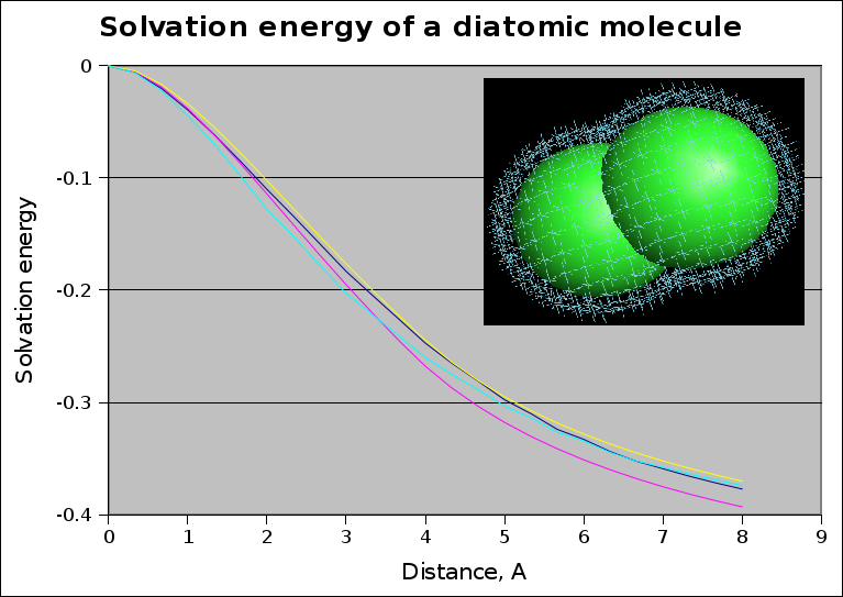
Figure 7: Solvation energy of a diatomic molecule (in units of $1389\,kJ\cdot\text{\AA}/(mol\cdot e^{2})$) for zero total charge.

The electrostatic part of the solvation energy corresponds to the blue curve of the previous graph and is calculated either by a (surface-electrostatic) Poisson equation solver (blue), FSBE (cyan), AGBNP (yellow) and HCT GB model (yellow). As it is clear from here, all the approaches give very similar results for the "small" molecule and are practically indistinguishable. Indeed, it is well known that practically any sort of GB approximation gives good results for solvation energies of small molecules.

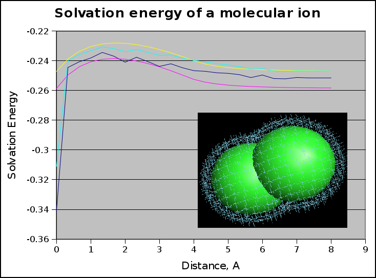
Figure 8: Solvation energy of a diatomic molecule of total charge 1 in units of $1389\,kJ\cdot\text{\AA}/(mol\cdot e^{2})$.

The difference between FSBE method and "classic" GB approaches and its relation to the exact solution becomes more obvious if we consider a charged diatomic molecule, namely, a molecular ion with total charge, say, 1 placed on one of the atoms (see Fig.8). The exact (blue) and FSBE (cyan), once again, are both in agreement with each other, whereas both "classic" GB approaches, HCT and AGBNP fail to recover correct asymptotic value at zero inter-atomic separation. The latter difference between GB solutions and the exact value of the solvation energy is not important for small molecules (low atom density) but is extremely important for macromolecules simulations and ligand binding calculations.

Binding energy calculations of a small molecule to a large protein often pose a difficult problem: a method for molecular electrostatic energy calculation should work well both for the protein ligand complex, the protein and the ligand at infinite separation. The protein and the complex are normally large molecules, whereas the ligand is, by definition, small. Not every computational approach for the solvation energy calculation is fit for the job though. To elucidate the nature of the problems at hand we performed another model calculation. First we prepared a spherical "protein" of a large (but realistic) radius. Then we placed a single-atom ligand with a charge at a given distance from the "protein" center as shown at the insets to Figures 9 and 10. Then we calculated the solvation energy of the system as a function of the ligand distance both when the protein is neutral and charged (in the latter case the protein charge was taken opposite to that of the "ligand")

Once again we used four different methods for the electrostatic contribution to the solvation energy calculation: a Poisson equation solver (in its surface electrostatic incarnation, blue), FSBE (cyan) and the two "classic" GB methods, based on the Coulomb approximation: HCT (magenta) and AGBNP (yellow).

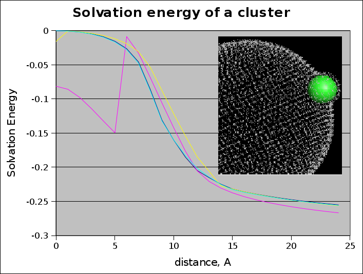
Figure 9: Solvation energy of a cluster of total charge 0 (units as in Figs.6,7,8).

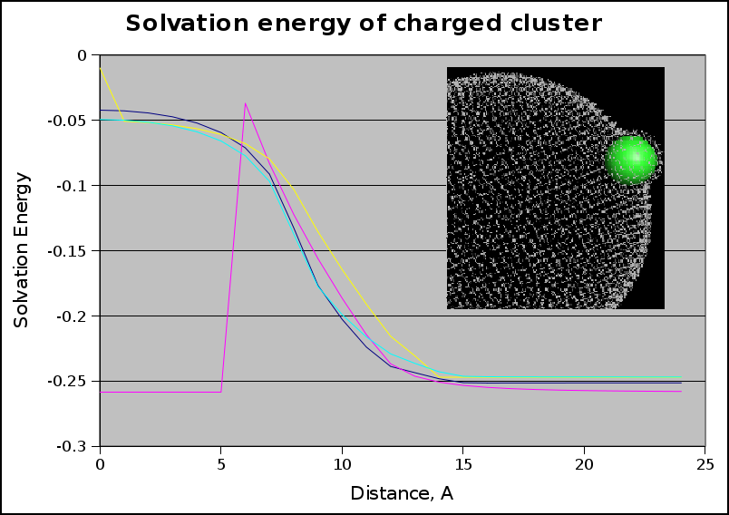
Figure 10: Solvation energy of a cluster of total charge 1 (units as in Figs.6,7,8).

Fig. 9 corresponds to an overall electrically neutral cluster and shows absolute deficiency of HCT approach deep enough inside the "protein". The problem is caused by unrealistic assumptions with regard to the overlap integrals calculations is occurs pretty frequently in realistic proteins. AGBNP method represents one of the latest and possibly the best among GB approaches. In fact the method is specifically designed to account for the atoms overlap better and ease the problem. However, AGBNP is based on Coulomb approximation and thus fails to recover correct behavior of the solvation energy close to the "protein" boundary: AGBNP energy is off by a large number from both FSBE and the exact solution. Remarkably, the FSBE and Poisson solutions agree very well everywhere. Fig.10 shows the same calculation for a charged model "protein-ligand" complex. Once again, HCT fails entirely, AGBNP does not work properly at the "protein" boundary and both the Poisson solver and FSBE agree very well, though FSBE does not require iterations and hence is about one order of magnitude faster than a FEM Poisson equation solver.

The results presented in this Section so far may be fine but concern only a few oversimplified examples produced for model systems with idealized geometries. To judge on actual performance of the method we turn to a practically interesting realistic system: solvation energy calculations for $N8$-neuraminidase protein (pdb accession code $2ht7$). The molecule is composed of 387 amino acids and, after all the hydrogen atoms added, has 5866 atoms. The results of the calculations are represented on Fig. 11. The horizontal axis represents the Born radii obtained “exactly” by solving surface boundary condition version of the Poisson equation as described by Eq. (3). The vertical axis shows the Born radii subsequently obtained by “standard” CA GB method in its surface incarnation (12), FSBE and our in house realization of AGBNP. Both the surface Born and FSBE calculations were performed using the same surface generated using the same set of (realistic) atom radii. The solid dots very next to the diagonal correspond to FSBE results. The values obtained with the standard Generalized Born approximation are depicted by the turned crosses and generally lay above the “exact” results. At last, the AGBNP results are given by the crosses at the bottom of the Figure.

The results of the calculation support every statement we made and hopes we put in designing FSBE method. AGBNP does not work well since its pair approximation to the overlap integrals estimation does not hold for a densely packed atom ensemble, such as a realistic protein exactly in the same way as it happened in our model spherical “protein” calculation discussed earlier in this paper and presented on Fig. 5. It is not a specific AGBNP fault, in fact any method based on pairwise descreening estimations would perform similarly. FSBE appears to fair very well especially when the Born radii are small which is indicative to atoms next to the protein surface, where normally all the ions are and most of interesting interactions, such as protein-ligand coupling occur. Standard GB in CA fails to reproduce Born radii values smaller than $10\textrm{\AA}$. In fact the radii calculated in CA are two times larger than those obtained with FSBE or the exact values. It is exactly the behavior we expected from our earlier sphere model discussion (see Fig. 2). The Figure also shows that neither FSBE results are perfect. Nevertheless FSBE is clearly superior to surface GB in CA, provides better both quantitative (at low Born radii values) and qualitative agreement with the exact results. The apparent deficiency of the method for large Born radii is also explainable: large $R_{B}$ correspond to deeply buried atoms, which is exactly the situation when FSBE results deviate from the exact solution most. We note that FEM such as SES are merely attempts to solve electrostatics problem in a complicated molecular geometry and may be sometimes produce wrong energies due to its own method specific problems.

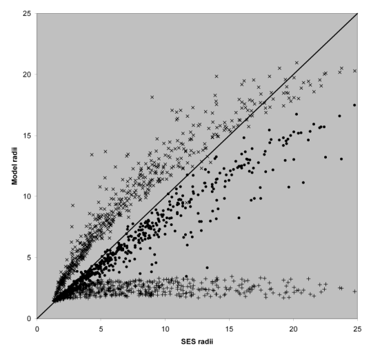
Figure 11: Born radii calculation as a comparison of different GB methods performance vs. “exact” Poisson equation solver. The atoms position were taken from a crystallized structure of $N8$ neuraminidase (pdb accession code $2ht7$). The dots, the turned and the standard crosses correspond to FSBE, surface GB in CA and a volume integral with pair overlaps estimation (AGBNP).

V Conclusions

The results and the analysis above suggest that our FSBE approach represents a fast and fairly accurate approximation to the Poisson equation solution. FSBE approach does not rely on Coulomb approximation (CA) and is shown to work well both for small molecules and large molecular clusters involving molecules of very different sizes. Therefore, FSBE has a potential to compute solvation energies with a single transferable set of GB parameters capable of describing correct dissociation limit of large and small molecules on the same footing.

FSBE is conceptually simple and shares the best of the two words: the calculation speed and smoothness of the energy surface of GB models and accuracy of FEM. Therefore the approximation should become a weapon of choice for a (relatively) fast calculation of solvation energies in modeling. FSBE is not a rigorous variational solution to the Poisson equation and can therefore be further improved. Neither FSBE is the only possible way to get rid of CA. As suggested earlier, both FSBE and even “classic” GB can be viewed as a variational approach with, e.g., single-parameter probe function of the kind:

$$\frac{1}{\left[R\left(\mathbf{r}\right)\right]^{\alpha}}=C_{\alpha}\int_{\Gamma_{W}}\frac{1}{\left|\mathbf{r^{\prime}}-\mathbf{r}\right|^{\alpha+2}}df^{\prime},$$ (29)

where $\alpha$ is the variational parameter, and $C_{\alpha}$ is a simple geometric factor, depending on the choice of $\alpha$. We were able to find, that essentially more exact expression (we call it as the “FSBE improved”, or FSBEi approach) can be obtained with $\alpha=2$, i.e. when

$$\frac{1}{R_{i}^{2}}=\frac{1}{4\pi}\int_{\Gamma_{W}}\frac{df^{\prime}}{s_{i}^{4}}.$$ (30)

Figs. 3 and 4 demonstrate that FSBEi turns out to be even more accurate and stable than FSBE in our simplified model example calculations. Unfortunately we were not able to obtain analytical derivatives $\partial R_{i}/\partial\mathbf{r}_{j}$ for the radii from Eq. (30) for the specific surface implementation we use. Nevertheless, the FSBE in the form presented here gives accurate enough for practical applications values of solvation energies. Moreover in typical situations such as in proteins ions normally sit next to the water interfaces, and therefore, the resulting error for solvation energy is small.

The idea to use integrals of the form of Eq. (29) in either volume or surface integral formulation to improve the accuracy of GB is not new (Ghosh et al., 1998; Romanov et al., 2004). It was suggested that a linear combination of properly chosen integrals of the form of Eq. (29) with adjustable coefficients leads to a transferable (from small to big molecules) method. Nevertheless, such an approach does not let one to select a specific model (most of the models studied by the authors have similar errors when compared with the exact solution). We argue that FSBE method presented here gives a unique approximation as a unique solution of the variational problem.

FSBE has even more of subtle advantages over current GB approximations. We do not have exponential extrapolation factors in the denominator of Eq.(10) and thus are able to compute FSBE solvation energies considerably faster. FSBE lets us compute polarization surface charge density from Eq.(24) and hence obtain the solvation energy in essentially $O(N)$ time and memory, as described in our subsequent work (Fedichev et al., 2009). The deficiencies of the method, such as its (relative) failure to get large values of Born radii right, as well as its possible improvements, such as FSBEi, are left for future work.

With all the apparent success of the method in solving the electrostatics problem, its applications to biomolecules modeling is limited by the fact, that water is not a simple dielectric with local and large value of the dielectric constant. The Poisson equation can describe neither volume or surface phase transitions and hydrogen bonds networks rearrangements (Fedichev and Menshikov, 2008; Menshikov and Fedichev, 2009) nor water molecule orientational interactions in a polar liquid (Fedichev and Menshikov, 2009). Nevertheless, the idea to prescribe Born approximation a variational interpretation may serve as a universal framework to generate approximate solutions of arbitrary partial differential equations, including those of more sophisticated water models, such as (Fedichev and Menshikov, 2006).