Renormalization and resolution of singularities

Abstract.

Since the seminal work of Epstein and Glaser it is well established that perturbative renormalization of ultraviolet divergences in position space amounts to extension of distributions onto diagonals. For a general Feynman graph the relevant diagonals form a nontrivial arrangement of linear subspaces. One may therefore ask if renormalization becomes simpler if one resolves this arrangement to a normal crossing divisor. In this paper we study the extension problem of distributions onto the wonderful models of de Concini and Procesi, which generalize the Fulton-MacPherson compactification of configuration spaces. We show that a canonical extension onto the smooth model coincides with the usual Epstein-Glaser renormalization. To this end we use an analytic regularization for position space. The ’t Hooft identities relating the pole coefficients may be recovered from the stratification, and Zimmermann’s forest formula is encoded in the geometry of the compactification. Consequently one subtraction along each irreducible component of the divisor suffices to get a finite result using local counterterms. As a corollary, we identify the Hopf algebra of at most logarithmic Feynman graphs in position space, and discuss the case of higher degree of divergence.

1. Introduction

The subject of perturbative renormalization in four-dimensional interacting quantum field theories looks back to a successful history. Thanks to the achievements of Bogoliubov, Hepp, Zimmermann, Epstein, Glaser, ’t Hooft, Veltman, Polchinski, Wilson – to mention just some of the most prominent contributors –, the concept seems in principle well-understood; and the predictions made using the renormalized perturbative expansion match the physics observed in the accelerators with tremendous accuracy. However, several decades later, our understanding of realistic interacting quantum field theories is still everything but satisfying. Not only is it extremely difficult to perform computations beyond the very lowest orders, but also the transition to a non-perturbative framework and the incorporation of gravity pose enormous conceptual challenges.

Over the past fifteen years, progress has been made, among others, in the following three directions. In the algebraic approach to quantum field theory, perturbation theory was generalized to generic (curved) space-times by one of the authors and Fredenhagen [BF], see also [HollandsWald]. On the other hand, Connes and one of the authors introduced infinite-dimensional Hopf- and Lie algebras [Kreimer, CK2] providing a deeper conceptual understanding of the combinatorial and algebraic aspects of renormalization, also beyond perturbation theory. More recently, a conjecture concerning the appearance of a very special class of periods [Broadhurst-Kreimer-96-2, BroadKreimer3, BB] in all Feynman integrals computed so far, has initiated a new area of research [BEK, BlochJapan, BlKr] which studies the perturbative expansion from a motivic point of view. The main purpose of this paper is to contribute to the three approaches mentioned, by giving a description of perturbative renormalization of short-distance divergences using a resolution of singularities. For future applications to curved spacetimes it is most appropriate to do this in the position space framework of Epstein and Glaser [EG, BF]. However the combinatorial features of the resolution allow for a convenient transition to the momentum space picture of the Connes-Kreimer Hopf algebras, and to the residues of [BEK, BlKr] in the parametric representation. Both notions are not immediately obvious in the original Epstein-Glaser literature.

Let us present some of the basic ideas in a nutshell. Consider, in euclidean space-time $M=\mathbb{R}^{4},$ the following Feynman graph

$$\Gamma=\;\raisebox{-22.76228pt}{\epsfbox{4pts-einer.eps}}\;.$$

The Feynman rules, in position space, associate to $\Gamma$ a distribution

$$u_{\Gamma}(x_{1},x_{2})=u_{0}^{2}(x_{1}-x_{2}).$$

where $u_{0}(x)$ is the Feynman propagator, in the massless case $u_{0}(x)=1/x^{2},$ the $x$ are 4-vectors with coordinates $x^{0},\ldots,x^{3},$ and $x^{2}$ the euclidean square $x^{2}=(x^{0})^{2}+\ldots+(x^{3})^{2}.$ Note that since $u_{\Gamma}$ depends only on the difference vector $x_{1}-x_{2},$ we may equally well consider $\underline{u}_{\Gamma}(x)=u_{\Gamma}(x,0).$ Because of the singular nature of $u_{0}$ at $x=0,$ the distribution $u_{\Gamma}$ is only well-defined outside of the diagonal $D_{12}=\{x_{1}=x_{2}\}\subset M^{2}.$ In order to extend $u_{\Gamma}$ from being a distribution on $M^{2}-D_{12}$ onto all of $M^{2},$ one can introduce an analytic regularization, say

$$\underline{u}_{\Gamma}^{s}(x)=u_{0}^{2s}(x).$$

Viewing this as a Laurent series in $s,$ we find, in this simple case,

$$\underline{u}_{\Gamma}^{s}(x) = \frac{1}{x^{4s}}=\frac{c\delta_{0}(x)}{s-1}+R_{s}(x)$$

with $c\in\mathbb{R},$ $\delta_{0}$ the Dirac measure at $0,$ and $s\mapsto R_{s}$ a distribution-valued function holomorphic in a complex neighborhood of $s=1,$ the important point being that the distribution $R_{s}$ is defined everywhere on $M^{2}.$ The usual way of renormalizing $\underline{u}_{\Gamma}$ is to subtract from it a distribution which is equally singular at $x=0$ and cancels the pole, for example

$$\underline{u}_{\Gamma,R}=\left.\left(\underline{u}^{s}_{\Gamma}-\underline{u}^{s}_{\Gamma}[w_{0}]\delta_{0}\right)\right|_{s=1}.$$

Here $w_{0}$ is any test function which satisfies $w_{0}(0)=1$ for then $\frac{\delta_{0}}{s-1}[w_{0}]=\frac{1}{s-1}.$ Consequently

$$\underline{u}_{\Gamma,R}=R_{1}-R_{1}[w_{0}]\delta_{0}$$

which is well-defined also at $0.$ The distribution $\underline{u}_{\Gamma,R}$ is considered the solution to the renormalization problem for $\Gamma,$ and different choices of $w_{0}$ give rise to the renormalization group. Once the graph $\Gamma$ is renormalized, there is a canonical way to renormalize the graph

$$\Gamma^{\prime}=\;\raisebox{-22.76228pt}{\epsfbox{4pts-disj.eps}}\;$$

which is simply a disjoint union of two copies of $\Gamma$. Indeed,

$$u_{\Gamma^{\prime}}(x_{1},x_{2},x_{3},x_{4})=u_{0}^{2}(x_{1}-x_{2})u_{0}^{2}(x_{3}-x_{4})=(\underline{u}_{\Gamma}\otimes\underline{u}_{\Gamma})(x_{1}-x_{2},x_{3}-x_{4}).$$

In other words, $u_{\Gamma^{\prime}}$ is a cartesian product, and one simply renormalizes each factor of it separately: $(u_{\Gamma^{\prime},R})(x_{1},\ldots,x_{4})=\underline{u}_{\Gamma,R}^{\otimes 2}(x_{1}-x_{2},x_{3}-x_{4}).$ This works not only for disconnected graphs but for instance also for

$$\Gamma^{\prime\prime}=\;\raisebox{-22.76228pt}{\epsfbox{4pts-reduzwei.eps}}\;$$

which is connected but (one-vertex-) reducible, to be defined later. Indeed,

$$u_{\Gamma^{\prime\prime}}(x_{1},x_{2},x_{3},x_{4}) = u_{0}^{2}(x_{1}-x_{2})u_{0}^{2}(x_{2}-x_{4})u_{0}^{2}(x_{3}-x_{4})$$

$$= \underline{u}_{\Gamma}^{\otimes 3}(x_{1}-x_{2},x_{2}-x_{4},x_{3}-x_{4})$$

Again, one simply renormalizes every factor of $u_{\Gamma^{\prime\prime}}$ on its respective diagonal. This is possible because the diagonals $D_{12},$ $D_{24}$ and $D_{34}$ are pairwise perpendicular in $M^{4}.$ Consider now a graph which is not of this kind:

$$\Gamma^{\prime\prime\prime}=\;\raisebox{-21.33955pt}{\epsfbox{4pts-gamma5.eps}}\;$$

$$u_{\Gamma^{\prime\prime\prime}}(x_{1},\ldots,x_{4})=u_{0}(x_{1}-x_{2})u_{0}(x_{1}-x_{3})u_{0}(x_{2}-x_{3})u_{0}(x_{2}-x_{4})u_{0}^{2}(x_{3}-x_{4}).$$

By the usual power counting we see that $u_{\Gamma^{\prime\prime\prime}}$ has non-integrable singularities at $D_{34}=\{x_{3}=x_{4}\},$ at $D_{234}=\{x_{2}=x_{3}=x_{4}\}$ and at $D_{1234}=\{x_{1}=x_{2}=x_{3}=x_{4}\}.$ These three linear subspaces of $M^{4}$ are nested $(D_{1234}\subset D_{234}\subset D_{34})$ instead of pairwise perpendicular. In the geometry of $M^{4}$ it does not seem possible to perform the three necessary subtractions separately and independently one of another. For if a test function has support on some of say $D_{1234},$ its support intersects also $D_{234}\setminus D_{1234}$ and $D_{34}\setminus D_{234}.$ This is one of the reasons why much literature on renormalization is based on recursive or step-by-step methods. If one instead transforms $M^{4}$ to another smooth manifold $\beta:Y\rightarrow M^{4}$ such that the preimages under $\beta$ of the three linear spaces $D_{34},D_{234},D_{1234}$ look locally like an intersection of three cartesian coordinate hyperplanes $y_{1}y_{2}y_{3}=0,$ one can again perform the three renormalizations separately, and project the result back down to $M^{4}.$ For this procedure there is no recursive recipe needed – the geometry of $Y$ encodes all the combinatorial information. The result is the same as from the Epstein-Glaser, BPHZ or Hopf algebra methods, and much of our approach just a careful geometric rediscovery of existing ideas.

In section 2 the two subspace arrangements associated to a Feynman graph are defined, describing the locus of singularities, and the locus of non-integrable singularities, respectively. In section 3 an analytic regularization for the propagator is introduced. Some necessary technical prerequisites for dealing with distributions and birational transformations are made, and the important notion of residue density for a primitive graph is defined. The rest of the paper is devoted to a more systematic development. Section 4 describes the De Concini-Procesi ”wonderful” models for the subspace arrangements and provides an explicit atlas and stratification for them in terms of nested sets. Different models are obtained by varying the so-called building set, and we are especially interested in the minimal and maximal building set/model in this class. Section 5 examines the pullback of the regularized Feynman distribution onto the smooth model and studies relations between its Laurent coefficients with respect to the regulator. In section 6 it is shown that the proposed renormalization on the smooth model satisfies the physical constraint of locality: the subtractions made can be packaged as local counterterms into the Lagrangian. For the model constructed from the minimal building set, this is satisfied by construction. From the geometric features of the smooth models one arrives quickly at an analogy with the Hopf algebras of Feynman graphs, and a section relating the two approaches concludes the exposition. As a technical simplication in the main part of the paper only massless scalar euclidean theories are considered, and only Feynman graphs with at most logarithmic singularities. The general case is briefly discussed in section 6.4. Questions of renormalization conditions, and the renormalization group, are left for future research.

This research is motivated by a careful analysis of Atiyah’s paper [Atiyah] – see also [BG]; and [BB2] for a first application to Feynman integrals in the parametric representation – the similarity of the Fulton-MacPherson stratification with the Hopf algebras of perturbative renormalization observed in [Kreimer3, Diplom], and recent results on residues of primitive graphs and periods of mixed Hodge structures [BlochJapan, BEK]. Kontsevich has pointed out the relevance of the Fulton-MacPherson compactification for renormalization long ago [Kontsevichtalk], and a real (spherical) version had been independently developed by him (and again independently by Axelrod and Singer [AS]) in the context of Chern-Simons theory, see for example [KontsevichEMS]. In the parametric representation, many related results have been obtained independently in the recent paper [BlKr], which provides also a description of renormalization in terms of limiting mixed Hodge structures. That is beyond our scope.

An earlier version of this paper has been presented in [Bergbauerthesis].

Acknowledgements

All three authors thank the Erwin Schrödinger Institut for hospitality during a stay in March and April 2007, where this paper has been initially conceived. C. B.  is grateful to K.  Fredenhagen, H.  Epstein, J.  Gracey, H.  Hauser, F.  Vignes-Tourneret, S.  Hollands, F.  Brown, E.  Vogt, C.  Lange, S.  Rosenberg, S.  Müller-Stach, S.  Bloch and H.  Gangl for general discussion. C. B.  is funded by the Deutsche Forschungsgemeinschaft, first under grant VO 1272/1-1 and presently in the SFB TR 45. He was supported by a Junior Fellowship while at ESI. He thanks the IHES, the Max-Planck-Institut Bonn and Boston University for hospitality and support during several stays in 2007 and 2008. D. K.  is supported by CNRS and in parts by NSF grant DMS-0603781. C. B.  and D. K.  thank the ESI for hospitality during another stay in March 2009.

2. Subspace arrangements associated to Feynman graphs

Let $U\subseteq\mathbb{R}^{k}$ be an open set. By $\mathcal{D}(U)=C^{\infty}_{0}(U)$ we denote the space of test functions with compact support in $U,$ with the usual topology. $\mathcal{D}^{\prime}(U)$ is the space of distributions in $U.$ See [Hoermander] for a general reference on distributions. We work in Euclidean spacetime $M=\mathbb{R}^{d}$ where $d\in 2+2\mathbb{N}=\{4,6,8,\ldots\}$ and use the (massless) propagator distribution

(1) $$u_{0}(x)=\frac{1}{x^{d-2}}=\frac{1}{((x^{0})^{2}+\ldots+(x^{d-1})^{2})^{\frac{d-2}{2}}}$$

which has the properties

(2) $$u_{0}(\lambda x)=\lambda^{2-d}u_{0}(x),\quad\lambda\in\mathbb{R}\setminus\{0\}$$

and

(3) $$\operatorname{sing}\operatorname{supp}u_{0}=\{0\}.$$

The singular support of a distribution $u$ is the set of points having no open neighborhood where $u$ is given by a $C^{\infty}$ function.

Let now $\Gamma$ be a Feynman graph, that is a finite graph, with set of vertices $V(\Gamma)$ and set of edges $E(\Gamma).$ We assume that $\Gamma$ has no loops (a loop is an edge that connects to one and the same vertex at both ends). The Feynman distribution is given by the distribution

(4) $$u_{\Gamma}(x_{1},\ldots,x_{n})=\prod_{i<j}u_{0}(x_{i}-x_{j})^{n_{ij}}$$

on $M^{n}\setminus\cup_{i<j}D_{ij}$ where $D_{ij}$ is the diagonal defined by $x_{i}=x_{j}$ and $n_{ij}$ is the number of edges between the vertices $i$ and $j$ (For this equation we assume that the vertices are numbered $V(\Gamma)=\{1,\ldots,n\}).$ A basic observation is that $u_{\Gamma}$ may be rewritten as the restriction of the distribution $u_{0}^{\otimes|E(\Gamma)|}\in\mathcal{D^{\prime}}(M^{|E(\Gamma)|})$ to the complement of a subspace arrangement, contained in a vector subspace of $M^{|E(\Gamma)|},$ as follows.

2.1. Configurations and subspace arrangements of singularities

It is convenient to adopt a more abstract point of view as in [BEK]. Let $E$ be a finite set and $\mathbb{R}^{E}$ the real vector space spanned by $E.$ If $V$ is a vector space we write $V^{\vee}$ for its dual space. Similarly, if $x\in V$ we write $x^{\vee}$ for the dual linear form. An inclusion of a linear subspace $i_{W}:W\hookrightarrow\mathbb{R}^{E}$ is called a configuration. Since $\mathbb{R}^{E}$ comes with a canonical basis, a configuration defines an arrangement of up to $|E|$ linear hyperplanes in $W:$ namely for each $e\in E$ the subspace annihilated by the linear form $e^{\vee}i_{W},$ unless this linear form equals zero. Note that different basis vectors $e\in E$ may give one and the same hyperplane.

Given a connected graph $\Gamma,$ temporarily impose an orientation of the edges (all results will be independent of this orientation). This defines for a vertex $v\in V(\Gamma)$ and an edge $e\in E(\Gamma)$ the integer $(v:e)=\pm 1$ if $v$ is the final/initial vertex of $e,$ and $(v:e)=0$ otherwise. The (simplicial) cohomology of $\Gamma$ is encoded in the sequence

(5) $$0\longrightarrow\mathbb{R}\stackrel{{\scriptstyle c}}{{\longrightarrow}}\mathbb{R}^{V(\Gamma)}\stackrel{{\scriptstyle\delta}}{{\longrightarrow}}\mathbb{R}^{E(\Gamma)}\longrightarrow H^{1}(\Gamma,\mathbb{R})\longrightarrow 0$$

with $c(1)=\sum_{v\in V(\Gamma)}v,$ $\delta(v)=\sum_{e\in E(\Gamma)}(v:e)e.$ This sequence defines two configurations: the inclusion of $\operatorname{coker}c$ into $\mathbb{R}^{E(\Gamma)},$ and dually the inclusion of $H_{1}(\Gamma,\mathbb{R})$ into $\mathbb{R}^{E(\Gamma)\vee}.$ We are presently interested in the first one, which corresponds to the position space picture.

It will be convenient to fix a basis $V_{0}$ of $\operatorname{coker}c.$ For example, the choice of a vertex $v_{0}\in V(\Gamma)$ (write $V_{0}=V(\Gamma)\setminus\{v_{0}\})$ provides an isomorphism $\phi:\mathbb{R}^{V_{0}}\rightarrow\operatorname{coker}c$ sending the basis element $v\in V_{0}$ to $v+\operatorname{im}c.$ We then have a configuration

(6) $$i_{\Gamma}=\delta\phi:\mathbb{R}^{V_{0}}\hookrightarrow\mathbb{R}^{E(\Gamma)}.$$

Each $e\in E(\Gamma)$ defines a linear form $e^{\vee}i_{\Gamma}\in(\mathbb{R}^{V_{0}})^{\vee}.$ It is non-zero since $\Gamma$ has no loops. Consider instead of $(\mathbb{R}^{V_{0}})^{\vee}$ the vector space $(M^{V_{0}})^{\vee}$ where $M=\mathbb{R}^{d}.$ For each $e\in E(\Gamma)$ there is a $d$-dimensional subspace

(7) $$A_{e}=(\operatorname{span}e^{\vee}i_{\Gamma})^{\oplus d}$$

of $(M^{V_{0}})^{\vee}.$ We denote this collection of $d$-dimensional subspaces of $(M^{V_{0}})^{\vee}$ by

(8) $$\mathcal{C}(\Gamma)=\{A_{e}:e\in E(\Gamma)\}.$$

Note that the $A_{e}$ need not be pairwise distinct nor linearly independent. By duality $\mathcal{C}(\Gamma)$ defines an arrangement of codimension $d$ subspaces in $M^{V_{0}}$

(9) $$M^{V_{0}}_{sing}(\Gamma)=\bigcup_{e\in E(\Gamma)}A_{e}^{\perp}$$

where $A_{e}^{\perp}$ is the linear subspace annihilated by $A_{e}.$ The image of $c^{\oplus d}$ in $M^{V(\Gamma)}$ is the thin diagonal $\Delta.$ It is in the kernel of all the $e^{\vee}i_{\Gamma},$ and therefore it suffices for us to work in the quotient space $\operatorname{coker}c.$ By construction $A_{e}^{\perp}=D_{jl}+\Delta$ where $j$ and $l$ are the boundary vertices of $e.$ In particular, if $\Gamma=K_{n}$ is the complete graph on $n$ vertices, then it is clear that $M^{V_{0}}_{sing}(K_{n})$ is the large diagonal $\bigcup_{j<l}D_{jl}+\Delta.$ The composition $\Phi:M^{V(\Gamma)}\rightarrow M^{V(\Gamma)}/\Delta\rightarrow M^{V_{0}}$ is given by $\Phi(x_{1},\ldots,x_{n})=(x_{1}-x_{n},\ldots,x_{n-1}-x_{n}),$ $x_{i}\in M,$ where again a numbering $V(\Gamma)=\{1,\ldots,n\},$ $v_{0}=n,$ of the vertices is assumed.

For a distribution $u$ on $M^{V}$ constant along $\Delta$ we write $\underline{u}=\Phi_{\ast}u$ for the pushforward onto $M^{V_{0}}.$ We usually write $(x_{1},\ldots,x_{n})$ for a point in $M^{\{1,\ldots,n\}},$ where $x_{i}$ is a $d$-tuple of coordinates $x_{i}^{0},\ldots,x_{i}^{d-1}$ for $M.$ Similarly, if $f\in(\mathbb{R}^{V_{0}})^{\vee}$ then $f^{0},\ldots,f^{d-1}$ are the obvious functionals on $M^{V_{0}}$ such that $f^{\oplus d}=(f^{0},\ldots,f^{d-1}).$

2.2. Subspace arrangements of divergences

Now we seek a refinement of the collection $\mathcal{C}(\Gamma)$ in order to sort out singularities where $u_{\Gamma}$ is locally integrable and does not require an extension. In a first step we stabilize the collection $\mathcal{C}(\Gamma)$ with respect to sums. Write

(10) $$\mathcal{C}_{sing}(\Gamma)=\left\{\sum_{e\in E^{\prime}}A_{e};\,\emptyset\subsetneq E^{\prime}\subseteq E(\Gamma)\right\}.$$

This is again a collection of non-zero subspaces of $(M^{V_{0}})^{\vee}.$ A subset $E^{\prime}$ of $E(\Gamma)$ defines a unique subgraph $\gamma$ of $\Gamma$ (not necessarily connected) with set of edges $E(\gamma)=E^{\prime}$ and set of vertices $V(\gamma)=V(\Gamma).$ Each subgraph $\gamma$ of $\Gamma$ determines an element

(11) $$A_{\gamma}=\sum_{e\in E(\gamma)}A_{e}$$

of $\mathcal{C}_{sing}(\Gamma).$ The map $\gamma\mapsto A_{\gamma}$ is in general not one-to-one.

Definition 2.1.

A subgraph $\gamma\subseteq\Gamma$ is called saturated if $A_{\gamma}\subsetneq A_{\gamma^{\prime}}$ for all subgraphs $\gamma^{\prime}\subseteq\Gamma$ such that $E(\gamma)\subsetneq E(\gamma^{\prime}).$

It is obvious that for any given $\gamma$ there is always a saturated subgraph, denoted $\gamma_{s},$ with $A_{\gamma}=A_{\gamma_{s}}.$ Also, $A_{e}\cap A_{\gamma_{s}}=\{0\}$ for all $e\in E(\Gamma)\setminus E(\gamma_{s}).$

Definition 2.2.

A graph $\Gamma$ is called at most logarithmic if all subgraphs $\gamma\subseteq\Gamma$ satisfy the condition $d\dim H_{1}(\gamma)-2|E(\gamma)|\leq 0.$

Definition 2.3.

A subgraph $\gamma\subseteq\Gamma$ is called divergent if $d\dim H_{1}(\gamma)=2|E(\gamma)|.$

Proposition 2.1.

Let $\Gamma$ be at most logarithmic. If $\gamma\subseteq\Gamma$ is divergent then it is saturated.

Proof. Assume that $\gamma$ satisfies the equality and is not saturated. Then there is an $e\in E(\gamma_{s})\setminus E(\gamma).$ Since $\gamma$ and $\gamma\cup\{e\}$ have the same number of components but $\gamma\cup\{e\}$ one more edge, it follows from (5) that $\dim H_{1}(\gamma\cup\{e\})=\dim H_{1}(\gamma)+1.$ Consequently, $d\dim H_{1}(\gamma\cup\{e\})=2|E(\gamma\cup\{e\})|+2$ in contradiction to $\Gamma$ being at most logarithmic. $\Box$

Let $\Gamma$ be at most logarithmic. We define

(12) $$\mathcal{C}_{div}(\Gamma)=\left\{A_{\gamma};\,\emptyset\subsetneq\gamma\subseteq\Gamma,\,\gamma\mbox{ divergent}\right\}$$

as a subcollection of $\mathcal{C}_{sing}(\Gamma).$ It is closed under sum (because $\dim H_{1}(\gamma_{1}\cup\gamma_{2})\geq\dim H_{1}(\gamma_{1})+\dim H_{1}(\gamma_{2})).$ It does not contain the space $\{0\}.$ In the dual, the arrangement

(13) $$M^{V_{0}}_{div}(\Gamma)=\bigcup_{\begin{array}[]{cc}\scriptstyle\emptyset\subsetneq\gamma\subseteq\Gamma\\ \scriptstyle d\dim H_{1}(\gamma)=2|E(\gamma)|\end{array}}A_{\gamma}^{\perp}$$

in $M^{V_{0}}$ describes the locus where extension is necessary:

Proposition 2.2.

Let $\Gamma$ be at most logarithmic. Then the largest open subset of $M^{V_{0}}\subset M^{E(\Gamma)}$ to which $u_{0}^{\otimes|E(\Gamma)|}$ can be restricted is the complement of $M^{V_{0}}_{div}(\Gamma).$ The restriction equals $\underline{u}_{\Gamma}$ there, and the singular support of $\underline{u}_{\Gamma}$ is the complement of $M^{V_{0}}_{div}(\Gamma)$ in $M^{V_{0}}_{sing}(\Gamma).$

Proof. Recall the map $i_{\Gamma}$ defining the configuration (6). It provides an inclusion $i_{\Gamma}^{\oplus d}:M^{V_{0}}\hookrightarrow M^{E(\Gamma)}.$ Wherever defined, $\underline{u}_{\Gamma}$ may be written $\underline{u}_{\Gamma}(x_{1},\ldots,x_{n-1})=\prod_{e\in E(\Gamma)}u_{0}\left(\sum_{v}(v:e)x_{v}\right)$ with $V_{0}=\{1,\ldots,n-1\}.$ Since $i_{\Gamma}(v)=\sum_{e}(v:e)e,$ in coordinates $i_{\Gamma}(\xi_{1},\ldots,\xi_{n-1})$ $=\left(\sum_{v}(v:e)\xi_{v}\right)_{e\in E(\Gamma)},$ it is clear that $\underline{u}_{\Gamma}=(i_{\Gamma}^{\oplus d})^{\ast}u_{0}^{\otimes|E(\Gamma)|}$ wherever it is defined. As by (3), $\operatorname{sing}\,\operatorname{supp}u_{0}=\{0\},$ the singular support of $u_{0}^{\otimes|E(\Gamma)|}$ is the locus where at least one $d$-tuple of coordinates vanishes: $x_{e}^{0}=\ldots=x_{e}^{d-1}=0$ for some $e\in E(\Gamma).$ Its preimage under $i_{\Gamma}^{\oplus d}$ is the locus annihilated by one of the $A_{e},$ whence the last statement. For the first statement, we have to show that for a compact subset $K\subset M^{V_{0}}$ the integral $\underline{u}_{\Gamma}|_{K}[\underline{1}]=\int_{K}\underline{u}_{\Gamma}(x)dx$ converges if and only if $K$ is disjoint from all the $A_{\gamma}^{\perp},$ for $\gamma\subseteq\Gamma$ such that $d\dim H_{1}(\gamma)=2|E(\gamma)|.$ Assume that $K\cap\left(A_{\gamma}^{\perp}\setminus\bigcup_{\gamma_{s}\subsetneq\gamma^{\prime}}A_{\gamma^{\prime}}^{\perp}\right)\neq\emptyset$ for some $\gamma.$ Write $\underline{u}_{\Gamma}=\prod_{e\in E(\gamma_{s})}u_{0}(\sum_{v}(v:e)x_{v})f$ where $f=\prod_{e\in E(\Gamma)\setminus E(\gamma_{s})}u_{0}(\sum_{v}(v:e)x_{v}).$ The distribution $f$ is $C^{\infty}$ on $A_{\gamma_{s}}^{\perp}\setminus\bigcup_{\gamma_{s}\subsetneq\gamma^{\prime}}A_{\gamma^{\prime}}^{\perp}$ since $A_{e}\cap A_{\gamma_{s}}=\{0\}$ for all $e\in E(\Gamma)\setminus E(\gamma_{s}).$ The integral $\int_{K}\underline{u}_{\Gamma}(x)dx$ is over a $d(n-1)$-dimensional space. The subspace $A_{\gamma_{s}}^{\perp}$ is given by $\dim A_{\gamma_{s}}$ equations. Each single $u_{0}(x)$ is of order $o(x^{2-d})$ as $x\rightarrow 0,$ and there are $|E(\gamma_{s})|$ of them in the first factor of $u_{\Gamma}.$ Hence the integral is convergent only if $\dim A_{\gamma_{s}}>(d-2)|E(\gamma_{s})|,$ which is the same as $2|E(\gamma_{s})|>d\dim H_{1}(\gamma_{s}).$ Conversely if this is the case for all $\gamma^{\prime}_{s}\subseteq\gamma_{s}$ then the integral is convergent. Our restriction to saturated subgraphs $\gamma_{s}$ is justified by Proposition 2.1. $\Box$

From now on through the end of section 5, $\Gamma$ is a fixed, connected, at most logarithmic graph. The general case where linear, quadratic, etc.  divergences occur is discussed in section 6.4.

2.3. Subspaces and polydiagonals

Let again $\gamma\subseteq\Gamma,$ that is $E(\gamma)\subseteq E(\Gamma)$ and $V(\gamma)=V(\Gamma).$ Recall from the end of section 2.1 that

(14) $$\Phi^{-1}(A_{\gamma}^{\perp})=\bigcap_{e\in E(\gamma)}D_{e}$$

with the diagonals $D_{e}=D_{jl}$ for $j$ and $l$ boundary vertices of $e.$ An intersection $\bigcap_{e\in E(\gamma)}D_{e}$ of diagonals is called a polydiagonal.

Just as in (5) we have an exact sequence

(15) $$0\longrightarrow H^{0}(\gamma,\mathbb{R})\stackrel{{\scriptstyle c_{\gamma}}}{{\longrightarrow}}\mathbb{R}^{V(\Gamma)}\stackrel{{\scriptstyle\delta_{\gamma}}}{{\longrightarrow}}\mathbb{R}^{E(\gamma)}\longrightarrow H^{1}(\gamma,\mathbb{R})\longrightarrow 0$$

with $c_{\gamma}$ sending each generator of $H^{0}(\gamma,\mathbb{R})$ (i. e. , a connected component $C$ of $\gamma$) to the sum of vertices in this component, $1_{C}\mapsto\sum_{v\in C}v$ and $\delta_{\gamma}(v)=\sum_{e\in E(\gamma)}(v:e)e.$ It is then a matter of notation to verify

Proposition 2.3.

(16) $$\Phi^{-1}(A_{\gamma}^{\perp})=\ker\delta_{\gamma}^{\oplus d}.$$

$\Box$

A polydiagonal $\Phi^{-1}(A_{\gamma}^{\perp})$ corresponds therefore to a partition $cc(\gamma)$ on the vertex set $V(\Gamma)$ as follows: $cc(\gamma)=\{Q_{1},\ldots,Q_{k}\}$ with pairwise disjoint cells $Q_{1},\ldots,Q_{k}\subseteq V(\Gamma)$ such that the vectors

(17) $$\sum_{v\in Q_{i}}v,\quad i=1,\ldots,k,$$

generate $\ker\delta_{\gamma}.$

In other words, $cc(\gamma)$ is the equivalence relation/partition ”connected by $\gamma$” on the set $V(\Gamma).$ If $\Gamma=K_{n}$ is the complete graph on $n$ vertices, this correspondence is clearly a bijection

(18) $$\{A_{\gamma}^{\perp}:\gamma\subseteq K_{n}\}\stackrel{{\scriptstyle\cong}}{{\rightarrow}}\{\mbox{ Partitions of }V(K_{n})\}.$$

The next proposition refines this statement. Recall our index notation from the end of section 2.1.

Proposition 2.4.

Let $\gamma,t\subseteq\Gamma.$ Then the set

(19) $$\mathcal{B}=\left\{(e^{\vee}i_{\Gamma})^{j}:e\in E(t),j=0,\ldots,d-1\right\}$$

is a basis of $A_{\gamma}$ if and only if $t$ is a spanning forest for $cc(\gamma),$

where a spanning forest is defined as follows.

Definition 2.4.

Let $\gamma,t\subseteq\Gamma.$ Then $t$ is a spanning forest for $cc(\gamma)$ if the map $\delta_{t}:\mathbb{R}^{V(\Gamma)}\rightarrow\mathbb{R}^{E(t)}$ as in (15) is surjective and $\ker\delta_{t}=\ker\delta_{\gamma}.$

Definition 2.5.

Let $\gamma,t\subseteq\Gamma$ and $t$ be a spanning forest for $cc(\gamma).$ If $t\subseteq\gamma$ then $t$ is a spanning forest of $\gamma.$ If $\gamma$ is connected (consequently so is $t$) then $t$ is called a spanning tree of $\gamma.$

In other words, a spanning forest of $\gamma$ is a subgraph of $\gamma$ without cycles that has the same connected components. A spanning forest for $cc(\gamma)$ has the same property but needs not be a subgraph of $\gamma.$

Proof of Proposition 2.4. By Proposition 2.3, $A_{\gamma}=A_{t}$ if and only if $\ker\delta_{\gamma}=\ker\delta_{t}.$ It remains to show that the set (19) is linearly independent if and only if $\delta_{t}$ is surjective. Since $\ker\delta_{\Gamma}\subseteq\ker\delta_{t}$ the map $\delta_{t}$ is surjective if and only if $i_{t}=\delta_{t}\phi:\mathbb{R}^{V_{0}}\rightarrow\mathbb{R}^{E(t)}$ (see (6)) is surjective, which in turn is equivalent to (19) having full rank, as $e^{\vee}i_{\Gamma}=e^{\vee}i_{t}$ for $e\in E(t).$ $\Box$

We also note two simple consequences for future use. Recall our definition of a subgraph $\gamma$ of $\Gamma:$ If $\Gamma$ is a graph with set of vertices $V(\Gamma)$ and set of edges $E(\Gamma),$ a subgraph $\gamma$ is given by a subset $E(\gamma)\subseteq E(\Gamma)$ of edges. By definition $V(\gamma)=V(\Gamma).$ However, we define $V_{\operatorname{eff}}(\gamma)$ to be the subset of vertices in $V(\gamma)$ which are not isolated – a vertex $v$ is not isolated if it is connected to another vertex through $\gamma.$ By abuse of language we say a proper subgraph $\gamma$ of $\Gamma$ is connected if it is connected as a graph with vertex set $V_{\operatorname{eff}}(\gamma)$ and edge set $E(\gamma),$ in other words, not taking the isolated vertices into account.

Proposition 2.5.

Let $\gamma_{1},\gamma_{2}\subseteq\Gamma,$ and assume $\gamma_{1}$ connected. Then

(20) $$A_{\gamma_{1}}\cap A_{\gamma_{2}}=A_{\gamma}$$

for any subgraph $\gamma$ of $\Gamma$ satisfying

(21) $$\operatorname{cc}(\gamma_{1})\cap\operatorname{cc}(\gamma_{2})=\operatorname{cc}(\gamma).$$

The intersection $P_{1}\cap P_{2}$ of partitions $P_{1},P_{2}$ on the same set $V(\Gamma)$ is defined by $P_{1}\cap P_{2}=\{Q_{1}\cap Q_{2}:Q_{1}\in P_{1},Q_{2}\in P_{2}\}.$ It is easily seen that this is a partition on $V(\Gamma)$ again. We write $0$ for the full partition $\{\{v\}:v\in V(\Gamma)\}.$

Proof. It is clear from Proposition 2.3 that

$$\Phi^{-1}((A_{\gamma_{1}}\cap A_{\gamma_{2}})^{\perp})=\ker\delta_{\gamma_{1}}^{\oplus d}+\ker\delta_{\gamma_{2}}^{\oplus d},$$

and one needs a partition $cc(\gamma)$ whose cells provide a basis as in (17) but now for the space $\ker\delta_{\gamma_{1}}+\ker\delta_{\gamma_{2}}.$ Let $cc(\gamma_{i})=\{Q_{1}^{i},\ldots,Q_{l_{i}}^{i}\}.$ Since

$$\sum_{v\in Q_{k}^{1}}v\in\operatorname{span}(\sum_{v\in Q_{k}^{1}\cap Q_{1}^{2}}v,\ldots,\sum_{v\in Q_{k}^{1}\cap Q_{l_{2}}^{2}}v),$$

and similarly for $1$ and $2$ interchanged, the vectors $\sum_{v\in Q_{k}^{1}\cap Q_{m}^{2}}v$ generate $\ker\delta_{\gamma_{1}}+\ker\delta_{\gamma_{2}}.$ Consequently, $\ker\delta_{\gamma_{1}}+\ker\delta_{\gamma_{2}}\subseteq\ker\delta_{\gamma}.$ In order to have equality, it suffices to show that the dimensions of both sides match. Since $\gamma_{1}$ is connected, we can assume $Q_{1}^{1}=\{1,\ldots,i\},$ $Q_{2}^{1}=\{i+1\},\ldots,Q^{1}_{n-i+1}=\{n\}.$ In that case clearly $\dim\ker\delta_{\gamma}=\dim H_{0}(\gamma)=|cc(\gamma_{1})\cap cc(\gamma_{2})|=|cc(\gamma_{1})|+\left|cc(\gamma_{2})|_{\{1,\ldots,i\}}\right|-1$ where $P|_{I}$ denotes the partition $\{Q\cap I,Q\in P\}.$ On the other hand one verifies that $\dim(\ker\delta_{\gamma_{1}}+\ker\delta_{\gamma_{2}})$ is the same. $\Box$

Apart from the intersection of partitions as defined above, it is useful to have the notion of a union of partitions. Let $cc(\gamma_{1}),cc(\gamma_{2})$ be partitions on $V(\Gamma).$ One defines most conveniently

(22) $$cc(\gamma_{1})\cup cc(\gamma_{2})=cc(\gamma_{1}\cup\gamma_{2}).$$

From the description before (18) it is clear that the right hand side in this definition depends only on $cc(\gamma_{1})$ and $cc(\gamma_{2})$ but not on $\gamma_{1}$ and $\gamma_{2}$ themselves. We immediately have

Proposition 2.6.

Let $\gamma_{1},\gamma_{2},\gamma\subseteq\Gamma.$ Then

(23) $$A_{\gamma_{1}}+A_{\gamma_{2}}=A_{\gamma}$$

if and only if

(24) $$\operatorname{cc}(\gamma_{1})\cup\operatorname{cc}(\gamma_{2})=\operatorname{cc}(\gamma).$$

$\Box$

It will be convenient later to have an explicit description of the dual basis $\mathcal{B}^{\vee},$ for $\mathcal{B}$ as in Proposition 2.4, that is the corresponding basis of $M^{V_{0}}.$ Recall our choice (above equation (6)) of a vertex $v_{0}$ in order to work modulo the thin diagonal. Recall also that the edges are oriented. Given a spanning tree $t$ of $\Gamma,$ we say $e\in E(t)$ points to $v_{0}$ if the final vertex of $e$ is closer to $v_{0}$ in $t$ than the initial vertex of $e.$ Otherwise we say that $e$ points away from $v_{0}.$ Furthermore, erasing the edge $e$ from $t$ separates $t$ into two connected components. The one not containing $v_{0}$ is denoted $t_{1},$ and we write $V_{\hat{e},0}=V_{\operatorname{eff}}(t_{1})$ for the set of its non-isolated vertices.

Proposition 2.7.

Let $\mathcal{B}^{\vee}=\{b^{j}_{e}:e\in E(t),j=0,\ldots,d-1\}$ be the basis of $M^{V_{0}}$ dual to a basis $\mathcal{B}$ of $(M^{V_{0}})^{\vee}$ as in Proposition 2.4 , that is $(e^{\vee}i_{\Gamma})^{j}(b^{k}_{e^{\prime}})=\delta_{e,e^{\prime}}\delta_{j,k}.$ Then

$$b_{e}=(-1)^{Q_{e}}\sum_{v\in V_{\hat{e},0}}v.$$

($V_{\hat{e},0},$ being a subset of the basis $V_{0}$ of $\mathbb{R}^{V_{0}},$ is also contained in $\mathbb{R}^{V_{0}}).$ We define $Q_{e}=\pm 1$ if $e$ points to/away from $v_{0}.$

Proof. Write $b_{e^{\prime}}=\sum_{v\in V_{0}}\beta^{e^{\prime}}_{v}v.$ We require

$$\delta_{e,e^{\prime}}=(e^{\vee}i_{\Gamma})(b_{e^{\prime}})=(e^{\vee}\delta\phi)(b_{e^{\prime}})=\sum_{v\in V_{0}}\beta^{e^{\prime}}_{v}(v:e).$$

Now fix an $e.$ Write $v_{in}(e),v_{out}(e)$ for the initial and final vertex of $e,$ respectively. We have $\beta^{e}_{v_{in}(e)}-\beta^{e}_{v_{out}(e)}=1$ and $\beta^{e}_{v_{in}(e^{\prime})}=\beta^{e}_{v_{out}(e^{\prime})}$ for the other edges $e^{\prime}$ except the one $e^{\prime}_{0}$ leading to $v_{0},$ for which $\beta^{e}_{v_{in}(e^{\prime}_{0})}=0$ or $\beta^{e}_{v_{out}(e^{\prime}_{0})}=0,$ depending on the direction of $e^{\prime}_{0}.$ Thus starting from $v_{0}$ and working one’s way along the tree $t$ in order to determine the $\beta^{e}_{v},$ all the $\beta^{e}_{v}=0$ until one reaches the edge $e,$ where $\beta^{e}_{v}$ jumps up or down to $1$ or $-1,$ depending on the orientation of $e,$ and stays constant then all beyond $e.$ $\Box$

Let us now describe the map $i_{\Gamma}^{\oplus d}:M^{V_{0}}\rightarrow M^{E(\Gamma)}$ in such a dual basis $\mathcal{B}^{\vee}.$ Let $x\in\mathbb{R}^{V_{0}},$ write $x=\sum_{e\in E(t)}x_{e}b_{e}$ with $b_{e}=(-1)^{Q_{e}}\sum_{v\in V_{\hat{e},0}}v$ as in Proposition 2.7. Write $[v_{i},v_{j}]\subseteq E(t)$ for the unique path in $t$ connecting the vertices $v_{i}$ and $v_{j}.$ It follows that

$$i_{\Gamma}(x)=\sum_{e\in E(\Gamma)}\sum_{v\in V_{0}}\sum_{e^{\prime}\in[v_{0},v]}(-1)^{Q_{e^{\prime}}}x_{e^{\prime}}(v:e)e.$$

For a given $e,$ only two vertices $v$ contribute to the sum, namely the boundaries $v_{in}(e)$ and $v_{out}(e)$ of $e.$ All the terms $(-1)^{Q_{e^{\prime}}}x_{e^{\prime}}$ for $e^{\prime}$ on the path from $v_{0}$ to $v_{in}(e)$ cancel since they appear twice, once with a negative sign $(v_{in}(e):e),$ once with a positive sign $(v_{out}(e):e).$ What remains are the terms on the path in $t$ from $v_{in}(e)$ to $v_{out}(e)$. We write $e^{\prime}\leadsto e$ if $e^{\prime}\in[v_{in}(e),v_{out}(e)]\subset E(t).$ Then

(25) $$i_{\Gamma}(x)=\sum_{e\in E(\Gamma)}\sum_{e^{\prime}\leadsto e}x_{e^{\prime}}e=\sum_{e\in E(t)}x_{e}e+\sum_{e\in E(\Gamma)\setminus E(t)}\sum_{e^{\prime}\leadsto e}x_{e^{\prime}}e.$$

Note that in the second sum there may be terms with only one $x_{e^{\prime}}$ contributing, namely when $A_{e}=A_{e^{\prime}}.$

3. Regularization, blowing up, and residues of primitive graphs

The purpose of this section is first to review a few standard facts about distributions and simple birational transformations. See [Hoermander] for a general reference on distributions. In the second part, the important notion of residue of a primitive Feynman graph is introduced by raising $u_{\Gamma}$ to a complex power $s$ in the neighborhood of $s=1$ and considering the residue at $s=1$ as a distribution supported on the exceptional divisor of a blowup.

3.1. Distributions and densities on manifolds

We recall basic notions that can be looked up, for example, in [Hoermander, Section 6.3]. When one wants to define the notion of distributions on a manifold one has two choices: The first is to model a distribution locally according to the idea that distributions are supposed to generalize $C^{\infty}$ functions, so they should transform like $u_{i}=(\psi_{j}\psi_{i}^{-1})^{\ast}u_{j}$ where $\psi_{i},\psi_{j}$ are two charts. On the other hand, distributions are supposed to be measures, that is one wants them to transform like $\tilde{u}_{i}=|\det\operatorname{Jac}\psi_{j}\psi_{i}^{-1}|(\psi_{j}\psi_{i}^{-1})^{\ast}\tilde{u}_{j}.$ The latter concept is called a distribution density.

By a manifold we mean a paracompact connected $C^{\infty}$ manifold throughout the paper. Let $\mathcal{M}$ be a manifold of dimension $m$ with an atlas $(\psi_{i},U_{i})$ of local charts $\psi_{i}:M_{i}\rightarrow U_{i}\subset\mathbb{R}^{m}.$

Definition 3.1.

A distribution $u$ on $\mathcal{M}$ is a collection $u=\{u_{i}\}$ of distributions $u_{i}\in\mathcal{D}^{\prime}(U_{i})$ satisfying

$$u_{i}=(\psi_{j}\psi_{i}^{-1})^{\ast}u_{j}$$

in $\psi_{j}(M_{i}\cap M_{j}).$ The space of distributions on $\mathcal{M}$ is denoted $\mathcal{D}^{\prime}(\mathcal{M}).$

Definition 3.2.

A distribution density $\tilde{u}$ on $\mathcal{M}$ is a collection $\tilde{u}=\{\tilde{u}_{i}\}$ of distributions $\tilde{u}_{i}\in\mathcal{D}^{\prime}(U_{i})$ satisfying

$$\tilde{u}_{i}=|\det\operatorname{Jac}\psi_{j}\psi_{i}^{-1}|(\psi_{j}\psi_{i}^{-1})^{\ast}\tilde{u}_{j}$$

in $\psi_{j}(M_{i}\cap M_{j}).$ The space of distribution densities on $\mathcal{M}$ is denoted $\mathcal{\tilde{D}}^{\prime}(\mathcal{M}).$ A density is called $C^{\infty}$ if all $\tilde{u}_{i}$ are $C^{\infty}.$ The space of $C^{\infty}$ densities on $\mathcal{M}$ with compact support is denoted $\tilde{C}^{\infty}_{0}(\mathcal{M}).$

Proposition 3.1.

1. ${C_{0}^{\infty}}^{\prime}(\mathcal{M})=\mathcal{\tilde{D}}^{\prime}(\mathcal{M}).$

2. $\tilde{C_{0}^{\infty}}^{\prime}(\mathcal{M})=\mathcal{D}^{\prime}(\mathcal{M}).$

3. A nowhere vanishing $C^{\infty}$ density $\alpha$ provides isomorphisms $u\mapsto u\alpha$ between $\mathcal{D}^{\prime}(\mathcal{M})$ and $\mathcal{\tilde{D}}^{\prime}(\mathcal{M}),$ and $C^{\infty}_{0}(\mathcal{M})$ and $\tilde{C}^{\infty}_{0}(\mathcal{M}),$ respectively.

$\Box$

$C^{\infty}$ densities are also called pseudo $m$-forms. If the manifold is oriented, every pseudo $m$-form is also a regular $m$-form, and conversely an $m$-form $\omega$ gives rise to two pseudo $m$-forms: $\omega$ and $-\omega.$ In a nonorientable situation we want to work with distribution densities and write them like pseudo forms $u(x)|dx|.$

3.2. Distributions and birational transformations

Let $\mathcal{M}$ be a manifold of dimension $m$ and $z\in\mathcal{M}$ a point in it. We work in local coordinates and may assume $\mathcal{M}=\mathbb{R}^{m}$ and $z=0.$ Blowing up $0$ means replacing $0$ by a real projective space $\mathcal{E}=\mathbb{P}^{m-1}(\mathbb{R})$ of codimension 1. The result is again a manifold as follows.

Let $Y=(\mathcal{M}\setminus\{0\})\sqcup\mathcal{E}$ as a set. Tangent directions at $0$ shall be identified with elements of $\mathcal{E}.$ Let therefore $Y^{\prime}$ be the subset of $\mathcal{M}\times\mathcal{E}$ defined by $z_{i}u_{j}=z_{j}u_{i},$ $1\leq i,j\leq m$ where $z_{1},\ldots,z_{m}$ are the affine coordinates of $\mathbb{R}^{m}$ and $u_{1},\ldots,u_{m}$ are homogeneous coordinates of $\mathbb{P}^{m-1}(\mathbb{R}).$ The set $Y^{\prime}$ is a submanifold of $\mathcal{M}\times\mathcal{E}.$ On the other hand, there is an obvious bijection $\lambda:Y\rightarrow Y^{\prime}$ whose restriction onto $\mathcal{M}\setminus\{0\}\subset Y$ is a diffeomorphism onto its image. Pulling back along $\lambda$ the differentiable structure induced on $Y^{\prime}$ defines a differentiable structure on all of $Y.$ The latter is called the blowup of $\mathcal{M}$ at $\{0\}.$ The submanifold $\mathcal{E}$ of $Y$ is called the exceptional divisor. There is a proper $C^{\infty}$ map $\beta:Y\rightarrow\mathcal{M}$ which is the identity on $\mathcal{M}\setminus\{0\}$ and sends $\mathcal{E}$ to $0.$ Viewed as a map from $Y^{\prime}\subset\mathcal{M}\times\mathcal{E},$ $\beta$ is simply the projection onto the first factor.

Note that if $m$ is even (which is the case throughout the paper) then $Y$ is not orientable but $\mathcal{E}$ is. If $m$ is odd then $Y$ is orientable but $\mathcal{E}$ is not. Indeed $Y$ is a fiber bundle $\tau:Y\rightarrow\mathcal{E}$ over $\mathcal{E}$ with fiber $\mathbb{R}$ – the tautological line bundle. For example, for $m=2,$ $Y$ is the open Möbius strip.

Let $m$ be even from now on. For $U_{i}=\mathbb{R}^{m},$ $i=1,\ldots,m,$ one defines maps $\rho_{i}:U_{i}\rightarrow\mathcal{M}\times\mathcal{E},$

$$(y_{1},\ldots,y_{m}) \mapsto ((z_{1},\ldots,z_{m}),[z_{1},\ldots,z_{m}])$$

$$z_{i}=(-1)^{i}y_{i},$$

$$z_{k}=y_{i}y_{k},\,k\neq i$$

where $z_{i}$ are coordinates on $\mathcal{M}$ and at the same time homogeneous coordinates for $\mathcal{E}.$ Clearly $\rho_{i}$ maps into $Y$ and onto the affine chart of $\mathcal{E}$ where $z_{i}\neq 0.$ Let $\psi_{i}=\rho_{i}^{-1}$ on $\rho_{i}(U_{i}).$ Then $(\psi_{i},U_{i})$ furnish an atlas for $Y.$ We note for future reference the transition maps

$$\psi_{j}\psi_{i}^{-1}: U_{i}\setminus\{y_{j}=0\}\rightarrow U_{j}\setminus\{y^{\prime}_{i}=0\}$$

$$(y_{1},\ldots,y_{m}) \mapsto (y^{\prime}_{1},\ldots,y^{\prime}_{m})$$

$$y^{\prime}_{i}=(-1)^{i+j}/y_{j},$$

$$y^{\prime}_{j}=(-1)^{j}y_{i}y_{j},$$

$$y^{\prime}_{k}=(-1)^{j}y_{k}/y_{j},\,k\neq i,j$$

and the determinants of their derivatives

(28) $$\det\operatorname{Jac}\psi_{j}\psi_{i}^{-1}=(-1)^{j+1}y_{j}^{1-m}.$$

Note that the atlas $(\psi_{i},U_{i})$ is therefore not even oriented on the open set $Y\setminus\mathcal{E}$ diffeomorphic to $\mathcal{M}\setminus\{0\}.$ For the exceptional divisor $\mathcal{E}=\mathbb{P}^{m-1}(\mathbb{R}),$ which is given in $U_{i}$ by the equation $y_{i}=0,$ we use induced charts $(\phi_{i},V_{i})$ with coordinates $y_{1},\ldots,\widehat{y_{i}},\ldots,y_{m}$ (in this very order) where $\widehat{y_{i}}$ means omission. The transition map

$$\phi_{j}\phi_{i}^{-1}: V_{i}\setminus\{y_{j}=0\}\rightarrow V_{j}\setminus\{y^{\prime}_{i}=0\}$$

$$(y_{1},\ldots,\widehat{y_{i}},\ldots,y_{m}) \mapsto (y^{\prime}_{1},\ldots,\widehat{y^{\prime}_{j}},\ldots,y^{\prime}_{m})$$

$$y^{\prime}_{i}=(-1)^{i+j}/y_{j},$$

$$y^{\prime}_{k}=(-1)^{j}y_{k}/y_{j},\,k\neq i,j$$

has Jacobian determinant

(30) $$\det\operatorname{Jac}\phi_{j}\phi_{i}^{-1}=y_{j}^{-m}>0.$$

The induced atlas $(V_{i},\phi_{i})$ is therefore an oriented one. The tautological bundle $\tau$ is given in local coordinates by $\tau:(y_{1},\ldots,y_{m})\mapsto(y_{1},\ldots,\widehat{y_{i}},\ldots,y_{m}).$

Similarly one defines blowing up along a submanifold: The submanifold is replaced by its projectivized normal bundle. Assume the submanifold is given in local coordinates by $z_{1}=\ldots=z_{k}=0.$ Then a natural choice of coordinates for the blowup is given again by (3.2), applied only to the subset of coordinates $z_{1},\ldots,z_{k}.$ See for instance [Mather, Section 3] for details.

The blowdown map $\beta:Y\rightarrow\mathcal{M}$ is surjective, proper and $C^{\infty}$ everywhere but open (i. e.  has surjective differential) only away from the exceptional divisor. It is called the blowdown map. It will be useful to be able to push distributions forward along $\beta$ and to pull distributions back along $\beta|_{Y\setminus\mathcal{E}}.$

In general, let $f:U\rightarrow V$ be a surjective proper $C^{\infty}$ map between open sets $U$ of $\mathbb{R}^{m_{1}}$ and $V$ of $\mathbb{R}^{m_{2}}.$ Let $u$ be a distribution on $U.$ The pushforward of $u$ by $f,$ denoted $f_{\ast}u,$ is the distribution on $V$ defined by $(f_{\ast}u)[\phi]=u[f^{\ast}\phi]$ where $\phi$ is a test function on $V$ and $f^{\ast}\phi$ is its pullback along $f:$ $f^{\ast}\phi=\phi\circ f.$ If $u$ has compact support the requirement that $f$ be proper can be dropped. Similarly, for $f:\mathcal{M}\rightarrow\mathcal{N}$ a surjective proper $C^{\infty}$ map between manifolds $\mathcal{M}$ and $\mathcal{N}$ with atlases $(\psi_{i},U_{i})$ and $(\theta_{i},V_{i}),$ let $u$ be a distribution density on $\mathcal{M}.$ Then $f_{\ast}u$ defined by

$$(f_{\ast}u)_{i}=(\theta_{i}f\psi^{-1}_{k})_{\ast}u_{k}$$

in $V_{i}\cap(\theta_{i}f\psi_{k}^{-1})(U_{k}),$ is a distribution density on $\mathcal{N}.$ Let now $f:\mathcal{M}\rightarrow\mathcal{N}$ a surjective $C^{\infty}$ map between manifolds $\mathcal{M}$ and $\mathcal{N}.$ It need not be proper. Let $u\in\mathcal{\tilde{D}}^{\prime}(\mathcal{M})$ and $\phi\in C^{\infty}_{0}(\mathcal{M}).$ The density $u[\phi]_{f}\in\mathcal{\tilde{D}}^{\prime}(\mathcal{N})$ is defined by

(31) $$u[\phi]_{f}=f_{\ast}(\phi u).$$

Note that $\phi u$ has compact support so the pushforward is well-defined although $f$ is not necessarily proper. If $u$ is given by a locally integrable function $u(z)$ on $\mathcal{M}=\mathbb{R}^{m}$ and $f$ is the projection onto $\mathcal{N}=\{z_{1},\ldots,z_{i}=0\}\subseteq\mathbb{R}^{m},$ $i<m,$ this notion corresponds to integrating out the orthogonal complement $\{z_{i+1},\ldots,z_{m}=0\}$ of $\mathcal{N}$ in $\mathbb{R}^{m}:$

$$u[\phi]_{f}(z_{i+1},\ldots,z_{m})=\int(u\phi)(z_{1},\ldots,z_{m})dz_{1}\ldots dz_{i}.$$

The reverse operation of pulling back distributions along $C^{\infty}$ maps is only possible under certain conditions, see [Hoermander, Sections 6.1, 8.2, etc.] for a general exposition. Here we only need the following simple case: Let $U_{1},U_{2}\subseteq\mathbb{R}^{n}$ open and $f:U_{1}\rightarrow U_{2}$ a $C^{\infty}$ and everywhere open map. Then there is a unique continuous linear map $f^{\ast}:\mathcal{D^{\prime}}(U_{2})\rightarrow\mathcal{D^{\prime}}(U_{1})$ such that $f^{\ast}u=u\circ f$ if $u\in C^{0}(U_{2}).$ See [Hoermander, Theorem 6.1.2] for a proof of this statement. It can obviously be generalized to the case of a submersion $f:\mathcal{M}\rightarrow\mathcal{N}$ of manifolds.

$\mathcal{M}=\mathbb{R}^{m}$ and its open subsets being orientable, distributions can be identified with distribution densities there, see Proposition 3.1 (iii). If $\beta$ is the blowdown map, by the pullback $\beta^{\ast}\tilde{u}$ of a distribution density $\tilde{u}\in\mathcal{\tilde{D}}^{\prime}(\mathcal{M}\setminus\{0\})$ obviously the pullback along the diffeomorphism $\beta|_{Y\setminus\mathcal{E}}$ is understood. The result is a distribution density on $Y\setminus\mathcal{E}.$

3.3. Analytic regularization

As a first step toward understanding $u_{\Gamma}^{s}$ as a distribution-valued meromorphic function of $s$ in a neighborhood of $s=1,$ we study distributions $u$ on $\mathbb{R}\setminus\{0\}$ of the form $u(z)=|z|^{-a}$ where $a\in\mathbb{Z}.$ Clearly if $a<1$ then $u\in L^{1}_{loc}(\mathbb{R}).$ The case $a\geq 1$ can be handled using analytic continuation with respect to the exponent: Let $a\in\mathbb{N}$ be fixed. We extend $u^{s}=|z|^{-as}$ meromorphically to the area $\Re s>1$ as follows. Let $n=\lfloor a/2\rfloor.$

$$u^{s}[\phi] = \int_{0}^{1}z^{-as}(\phi(z)+\phi(-z))dz+\int_{\mathbb{R}\setminus[-1,1]}|z|^{-as}\phi(z)dz$$

$$= \int_{0}^{1}z^{-as}\left(\phi(z)+\phi(-z)-2\left(\phi(0)+\ldots+\frac{z^{2n}\phi^{(2n)}(0)}{(2n)!}\right)\right)dz$$

$$+\int_{\mathbb{R}\setminus[-1,1]}|z|^{-as}\phi(z)dz+2\sum_{k=0}^{n}\frac{\phi^{(2k)}(0)}{(2k)!((2k+1)-as)}.$$

This holds for $\Re s<1+\frac{1}{a}.$ See [GS, Section I. 3] for the complete argument. There will be more poles beyond the half-plane $\Re s<1+\frac{1}{a}$ but they are not relevant for our purposes.

Definition 3.3.

The canonical regularization of $|z|^{-a}$ is the distribution-valued meromorphic function in $s\in(-\infty,1+\frac{1}{a})+i\mathbb{R}$ given by

(33) $$|z|_{ext}^{-as}=2\sum_{k=0}^{n}\frac{\delta_{0}^{(2k)}}{(2k)!((2k+1)-as)}+|z|_{fin}^{-as}$$

where $n=\lfloor a/2\rfloor$ and

(34) $$|z|_{fin}^{-as}[\phi] = \int_{0}^{1}z^{-as}\left(\phi(z)+\phi(-z)-2\left(\phi(0)+\ldots+\frac{z^{2n}\phi^{(2n)}(0)}{(2n)!}\right)\right)dz$$

$$+\int_{\mathbb{R}\setminus[-1,1]}|z|^{-as}\phi(z)dz.$$

The function $s\mapsto|z|_{fin}^{-as}$ is holomorphic in $(-\infty,1+\frac{1}{a})+i\mathbb{R}.$ When the context allows, we simply write $|z|^{-as}$ for $|z|^{-as}_{ext}$ again. Let $f\in C^{\infty}(\mathbb{R}).$ Since $s\mapsto f^{s}[\phi]$ is holomorphic, it makes sense to define the canonical regularization for $|z|^{-a}f$ also:

(35) $$(|z|^{-a}f)^{s}_{ext}=|z|^{-as}_{ext}\cdot f^{s}.$$

This does not work for $f\in L^{1}_{loc}(\mathbb{R}).$ For example, $|z|^{-(a+b)s}_{ext}\neq|z|^{-as}_{ext}|z|^{-bs}_{ext}.$

Unfortunately, the term ”regularization” is used for two different notions in the mathematics and physics literature, respectively. They must be carefully distinguished. While in the mathematics literature, the ”regularized” distribution is usually understood to be $|z|_{fin}^{-a},$ a physicist calls this the ”renormalized” distribution, and refers to the mapping $s\mapsto|z|^{-as}$ as a regularization (in fact, one out of many possible regularizations). The latter is also our convention.

We finally note the special case $a=1,$

(36) $$|z|_{ext}^{-s}=-\frac{2\delta_{0}}{s-1}+|z|_{fin}^{-s},$$

(37) $$|z|_{fin}^{-s}[\phi]=\int_{-1}^{1}|z|^{-s}(\phi(z)-\phi(0))dz+\int_{\mathbb{R}\setminus[-1,1]}|z|^{-s}\phi(z)dz.$$

And, for future reference, in the area $\Re s<\frac{2+(D-1)}{D},$

(38) $$|z|_{ext}^{D-Ds-1}=-\frac{2}{D}\frac{\delta_{0}}{s-1}+|z|_{fin}^{D-Ds-1}$$

where $D\in 2\mathbb{N}.$

3.4. Primitive graphs, their residues and renormalization

We consider the blowup $\beta:Y\rightarrow\mathcal{M}$ of $\mathcal{M}$ at 0 as in section 3.2 where now $\mathcal{M}=M^{V_{0}}$ for our Feynman graph $\Gamma$ (see section 2 for notation). Let $d_{\Gamma}=d|V_{0}|=\dim\mathcal{M}.$ In this section we continue to use the coordinates $z_{1},\ldots,z_{d_{\Gamma}}$ on $M^{V_{0}}$ and $y_{1},\ldots,y_{d_{\Gamma}}$ on the charts $U_{i}$ for $Y.$ They are related to the coordinates $x_{i}^{j}$ of section 2 by $x_{i}^{j}=z_{d(i-1)+j}.$ Recall that since $Y$ is not orientable (and the induced atlas on $Y\setminus\mathcal{E}$ is not oriented), top degree $(L^{1}_{loc})$ forms and distribution densities can not be identified. We only use forms on the oriented submanifold $\mathcal{E},$ where the two notions coincide. We write $|dz|$ for the Lebesgue measure on $\mathcal{M}.$

Definition 3.4.

A connected Feynman graph $\Gamma$ is called primitive if $\mathcal{C}_{div}(\Gamma)=\{A_{\Gamma}\}.$

Recall the notion of saturated subgraph from Definition 2.1 and Proposition 2.1.

Lemma 3.1.

Let $\Gamma$ be primitive. Let $t$ be a spanning tree for $\Gamma$ and $t^{\prime}$ a subgraph of $t.$ Then

$$d|E(t^{\prime})|\leq(d-2)(|E(\Gamma)|-|E((t\setminus t^{\prime})_{s})|)$$

and equality holds if and only if $t^{\prime}=t.$

Proof. Clearly $\dim A_{t}=\dim A_{t^{\prime}}+\dim A_{t\setminus t^{\prime}}$ and $\dim A_{t^{\prime}}=d|E(t^{\prime})|.$ Since $\Gamma$ is divergent, $(d-2)|E(\Gamma)|=\dim A_{t}.$ Since $\Gamma$ has no proper divergent subgraphs, $(d-2)|E((t\setminus t^{\prime})_{s})|<\dim A_{(t\setminus t^{\prime})_{s}}=\dim A_{t\setminus t^{\prime}}$ for all proper subgraphs $t^{\prime}$ of $t.$ $\Box$

Lemma 3.2.

Let $\delta_{\mathcal{E}}$ (resp.  $\frac{1}{|y_{\mathcal{E}}|})$ be collections of distributions in the $U_{i}$ given by $(\delta_{\mathcal{E}})_{i}=\delta_{0}(y_{i})$ and $(1/|y_{\mathcal{E}}|)_{i}=\frac{1}{|y_{i}|}$ in $U_{i}.$ Let $\omega$ be a locally integrable volume form $\omega$ on $\mathcal{E}.$ Then $\omega\delta_{\mathcal{E}}$ and $\omega/|y_{\mathcal{E}}|,$ locally

$$(\omega\delta_{\mathcal{E}})_{i} = \omega_{i}(\delta_{\mathcal{E}})_{i}=\omega_{i}(y_{1},\ldots,\widehat{y_{i}},\ldots,y_{d_{\Gamma}})\delta_{0}(y_{i}),$$

$$(\omega/|y_{\mathcal{E}}|)_{i} = \omega_{i}/|y_{\mathcal{E}}|_{i}=\omega_{i}(y_{1},\ldots,\widehat{y_{i}},\ldots,y_{d_{\Gamma}})/|y_{i}|$$

define densities on $Y.$

Proof. By (28) and (30) $|\operatorname{det}\operatorname{Jac}\psi_{j}\psi_{i}^{-1}|=\operatorname{det}\operatorname{Jac}\phi_{j}\phi_{i}^{-1}\cdot|1/y_{j}|$ and both $\delta_{0}$ and $1/|y_{i}|$ transform with the factor $|1/y_{j}|$ under transition $U_{i}\rightarrow U_{j}.$ $\Box$

Theorem 3.1.

Let $\Gamma$ be primitive.

1. By pullback along the diffeomorphism $\beta|_{Y\setminus\mathcal{E}},$ the distribution density $\tilde{u}_{\Gamma}=\underline{u}_{\Gamma}|dz|$ furnishes a strictly positive density $\tilde{w}_{\Gamma}$ on $Y\setminus\mathcal{E},$ given in local coordinates of $U_{i}$ by

   (39) $$(\tilde{w}_{\Gamma})_{i}|dy|=\frac{1}{|y_{i}|}(f_{\Gamma})_{i}(y_{1},\ldots,\widehat{y_{i}},\ldots,y_{d_{\Gamma}})|dy|$$

   where $(f_{\Gamma})_{i}\in L^{1}(V_{i}).$ The $(f_{\Gamma})_{i}\,dy_{1}\wedge\ldots\wedge\widehat{dy_{i}}\wedge\ldots\wedge dy_{d_{\Gamma}}$ in each $V_{i}$ determine an integrable volume form $f_{\Gamma}$ on $\mathcal{E}.$ We may therefore write $\tilde{w}_{\Gamma}=f_{\Gamma}/|y_{\mathcal{E}}|.$

2. The meromorphic density-valued function $s\mapsto\tilde{w}_{\Gamma}^{s}=\beta^{\ast}\tilde{u}_{\Gamma}^{s},$

   $$(\tilde{w}_{\Gamma}^{s})_{i}|dy|=\frac{(f_{\Gamma})_{i}^{s}|dy|}{|y_{i}|^{d_{\Gamma}s-(d_{\Gamma}-1)}}$$

   has a simple pole at $s=1.$ Its residue is the density

   (40) $$\operatorname{res}_{s=1}\tilde{w}_{\Gamma}^{s}=-\frac{2}{d_{\Gamma}}\delta_{\mathcal{E}}f_{\Gamma},$$

   supported on the exceptional divisor. Pushing forward along $\beta$ amounts to integrating a projective integral over the exceptional divisor:

   (41) $$\beta_{\ast}(\operatorname{res}_{s=1}\tilde{w}_{\Gamma}^{s})=-\frac{2}{d_{\Gamma}}\delta_{0}|dz|\int_{\mathcal{E}}f_{\Gamma}=-\frac{2}{d_{\Gamma}}\delta_{0}\int_{V_{i}}(f_{\Gamma})_{i}dy_{1}\ldots\widehat{dy_{i}}\ldots dy_{d_{\Gamma}}$$

   for any $i.$

3. Let $\mu\in\mathcal{D}(\mathbb{R}^{d_{\Gamma}})$ with $\mu(0)=1,$ and $\nu=\beta^{\ast}\mu.$ Let $\tau:Y\rightarrow\mathcal{E}$ be the tautological bundle. Then

   (42) $$\tilde{w}_{\Gamma,R}^{s}=\tilde{w}_{\Gamma}^{s}-\tilde{w}_{\Gamma}^{s}[\nu]_{\tau}\delta_{\mathcal{E}}$$

   defines a density-valued function on $Y$ holomorphic in a neighborhood of $s=1.$ Also $\beta_{\ast}\tilde{w}^{s}_{\Gamma,R}=(\underline{u}_{\Gamma}^{s}-\underline{u}_{\Gamma}^{s}[\mu]\delta_{0})|dz|=\underline{u}^{s}_{\Gamma,R}|dz|.$

The density (40) is called residue density, the volume form $f_{\Gamma}$ residue form, and the complex number

(43) $$\operatorname{res}\Gamma=-\frac{2}{d_{\Gamma}}\int_{\mathcal{E}}f_{\Gamma}$$

residue of $\Gamma.$ The distribution $\underline{u}_{\Gamma,R}=\underline{u}_{\Gamma,R}^{s}|_{s=1}$ is defined on all of $M^{V_{0}}$ and said to be the renormalized distribution.

Proof of Theorem 3.1. (i) For (39) observe that in local coordinates of $U_{i}$ the map $\beta$ is given by $\rho_{i},$ see (3.2). The Lebesgue measure $|dz|$ on $M^{V_{0}}$ pulls back to $|y_{i}|^{d_{\Gamma}-1}|dy|$ in $U_{i}.$ By (2), $\underline{u}_{\Gamma}$ scales like $\lambda^{(2-d)|E(\Gamma)|}$ as $z_{i}\rightarrow\lambda z_{i}$ for all $i.$ Since $\Gamma$ is divergent, $d_{\Gamma}=(2-d)|E(\Gamma)|,$ which explains the factor $1/|y_{i}|$ in (39) and that $(f_{\Gamma})_{i}$ does not depend on $y_{i}.$ That $(f_{\Gamma})_{i}\in L^{1}_{loc}(V_{i})$ follows from Proposition 2.2, where $M^{V_{0}}_{div}=A_{\Gamma}^{\perp}=\{0\},$ and $\beta|_{Y\setminus\mathcal{E}}$ being a diffeomorphism. In order to show that $(f_{\Gamma})_{i}\in L^{1}(V_{i})$ one uses Lemma 3.1 as follows: Choose a spanning tree $t$ for $\Gamma$ such that the coordinate $z_{i}$ equals $(e_{0}^{\vee}i_{\Gamma})^{j_{0}}$ for some $e_{0}\in E(t)$ and $j_{0}\in\{0,\ldots,d-1\}$ (see Proposition 2.4). Write $x_{e}^{j}=(e^{\vee}i_{\Gamma})^{j}$ for $e\in E(t),j=0,\ldots,d-1.$ In this basis $\underline{u}_{\Gamma}$ is given by $\underline{u}_{\Gamma}(\{x_{e}^{j}\})=\prod_{e\in E(\Gamma)}u_{0}(\sum_{e^{\prime}\leadsto e}x_{e^{\prime}}^{j})$ (see (25)). Therefore, if the coordinates $y_{e}^{j},\,e\in E(t^{\prime})\,j=0,\ldots,d-1$ defined by $t^{\prime}$ a proper subforest of $t$ not containing $e_{0}$ go to $\infty,$ then there are exactly $E(t_{s})\setminus E((t\setminus t^{\prime})_{s})$ factors of $u_{0}$ the argument of which goes to $\infty.$ Lemma 3.1 shows that the integration over that subspace converges. One verifies that all subspaces susceptible to infrared divergences are of this form. Therefore $(f_{\Gamma})_{i}\in L^{1}(V_{i}).$ Finally, the $(f_{\Gamma})_{i}$ produce a factor $y_{i}^{-d_{\Gamma}}$ under transition between charts. By (30) this makes $f_{\Gamma}$ a density on $\mathcal{E}.$ Since $\mathcal{E}$ is oriented, a strictly positive density is also a strictly positive ($L^{1}_{loc})$ volume form.
(ii) The simple pole and (40) follow from (39) by (38), the local expressions matched together using Lemma 3.2. For (41) let $\phi\in\mathcal{D}(M^{V_{0}}).$ Then $\beta_{\ast}(\operatorname{res}_{s=1}\tilde{w}^{s}_{\Gamma})[\phi]=\operatorname{res}_{s=1}\tilde{w}^{s}_{\Gamma}[\beta^{\ast}\phi].$ The distribution density $\operatorname{res}_{s=1}\tilde{w}^{s}_{\Gamma},$ being supported on $\mathcal{E},$ depends only on $\beta^{\ast}\phi|_{\mathcal{E}}=\phi(0).$ By the results of (i), $\int_{\mathcal{E}}f_{\Gamma}$ is a projective integral and it suffices to integrate inside one chart, say $U_{i}.$ There $\operatorname{res}_{s=1}\tilde{w}^{s}_{\Gamma}[\beta^{\ast}\phi]=-\frac{2}{d_{\Gamma}}\int_{U_{i}}\delta_{0}(y_{i})f_{\Gamma}(y)\phi(\rho_{i}(y))dy$ $=-\frac{2}{d_{\Gamma}}\phi(0)\int_{V_{i}}f_{\Gamma}(y)dy$ $=-\frac{2}{d_{\Gamma}}\phi(0)\int_{\mathcal{E}}f_{\Gamma}.$
(iii) There is no pole at $s=1$ since $\nu|_{\mathcal{E}}=1.$ The $(\tilde{w}^{s}_{\Gamma,R})_{i}$ furnish a density by Lemma 3.2: The Jacobian of $\delta_{\mathcal{E}}$ cancels the one of $[\ldots]_{\tau}.$ For the last statement, let again $(\psi_{i},U_{i})_{i=1,\ldots,d_{\Gamma}}$ be the chosen atlas for $Y$ and $(\phi_{i},V_{i})_{i=1,\ldots,d_{\Gamma}}$ the induced atlas for $\mathcal{E}.$ Since $\mathcal{E}$ is compact, there exists a partition of unity $(\xi_{i}\phi_{i})_{i=1,\ldots,d_{\Gamma}}$ on $\mathcal{E}$ subordinate to the $V_{i}$ such that $\xi_{i}\in\mathcal{D}(V_{i}),$ $\xi_{i}\geq 0$ and $\sum_{i}(\xi_{i}\phi_{i})(x)=1$ for all $x\in\mathcal{E}.$ Let $\tau:Y\rightarrow\mathcal{E}.$ Then $(\xi_{i}\phi_{i}\tau)_{i=1,\ldots,d_{\Gamma}}$ is a partition of unity on $Y$ subordinate to $(\psi_{i},U_{i})_{i=1,\ldots,d_{\Gamma}}$ (however not compactly supported). We fix such a partition of unity $(\xi_{i}).$ In $U_{i}$ we write $y$ for $(y_{1},\ldots,y_{d_{\Gamma}})$ and $\widehat{y_{i}}$ for $(y_{1},\ldots,\widehat{y_{i}},\ldots,y_{d_{\Gamma}}),$ for example $\xi_{i}(y)=\xi_{i}(\widehat{y_{i}})$ since it is constant along $y_{i}.$ We also write $u(y_{i},y_{i}\widehat{y_{i}})=u(y_{i}y_{1},\ldots,y_{i},\ldots,y_{i}y_{d_{\Gamma}})$ for convenience. Let $f\in\mathcal{D}(M^{V_{0}}).$

$$\beta_{\ast}(\tilde{w}^{s}_{\Gamma,R})[f] = \beta_{\ast}(\tilde{w}^{s}_{\Gamma}-\tilde{w}^{s}_{\Gamma}[\nu]_{\tau}\delta_{\mathcal{E}})[f]$$

$$= \sum_{i}(\tilde{w}^{s}_{\Gamma}-\tilde{w}_{\Gamma}^{s}[\nu]_{\tau}\delta_{\mathcal{E}})_{i}[\xi_{i}\beta^{\ast}f]$$

$$= \sum_{i}\int_{U_{i}}(\tilde{w}_{\Gamma}^{s}(y)-\int_{\mathbb{R}}\tilde{w}_{\Gamma}^{s}(z_{i},\widehat{y_{i}})\mu(z_{i},z_{i}\widehat{y_{i}})dz_{i}\delta_{0}(y_{i}))$$

$$\times\xi_{i}(y)f(y_{i},y_{i}\widehat{y_{i}})dy$$

$$= \sum_{i}\int_{U_{i}}\tilde{w}_{\Gamma}^{s}(y)\xi_{i}(y)f(y_{i},y_{i}\widehat{y_{i}})$$

$$-\tilde{w}_{\Gamma}^{s}(y)\mu(y_{i},y_{i}\widehat{y_{i}})\xi_{i}(0,\widehat{y_{i}})f(0)dy$$

$$= \sum_{i}(\beta_{\ast}\tilde{w}_{\Gamma}^{s}-\beta_{\ast}\tilde{w}_{\Gamma}^{s}[\xi_{i}\nu]\delta_{0})[f].$$

$\Box$

The following corollary concerns infrared divergences of a graph $\Gamma.$ Those are divergences which do not occur at the $A_{\gamma}^{\perp}$ but as the coordinates $z_{i}$ of $M^{V_{0}}$ approach $\infty,$ in other words, if one attempts to integrate $\underline{u}_{\Gamma}$ against a function which is not compactly supported.

Corollary 3.1.

Let $\Gamma$ be at most logarithmic and primitive. Then $\underline{u}_{\Gamma}$ is not (globally) integrable on $M^{V_{0}}\setminus M^{V_{0}}_{div}(\Gamma).$ However $(\chi\underline{u}_{\Gamma})[\underline{1}_{L}\otimes\mu]$ is well-defined, if $\mu$ is a test function on a non-zero subspace of $M^{V_{0}},$ $\underline{1}_{L}$ the constant function on the orthogonal complement $L,$ and $\chi$ the characteristic function of the complement of an open neighborhood of $M^{V_{0}}_{div}(\Gamma)$ in $M^{V_{0}}.$

Proof. This follows from part (i) of Theorem 3.1. $\Box$

The renormalized distribution $\underline{u}_{\Gamma,R}=\underline{u}_{\Gamma,R}^{s}|_{s=1}$ obtained from the theorem depends of course on $\mu.$ Write $\underline{u}_{\Gamma,R}$ for one using $\mu$ and $\underline{u}^{\prime}_{\Gamma,R}$ for another one using $\mu^{\prime},$ then the difference $\underline{u}_{\Gamma,R}-\underline{u}^{\prime}_{\Gamma,R}$ is supported on $0$ and of the form $c\delta_{0}$ with $c\in\mathbb{R}.$ This one-dimensional space of possible extensions represents the renormalization ambiguity.

Here is an example. Let $M=\mathbb{R}^{4}.$ For

$$\Gamma=\;\raisebox{-22.76228pt}{\epsfbox{4pts-einer.eps}}\;$$

we have

$$\underline{u}_{\Gamma}(x)=u_{0}^{2}(x)=1/x^{4},$$

the latter a distribution on $M^{V_{0}}\setminus\{0\}=M\setminus\{0\}.$ Pulling back along $\beta,$

$$(\beta^{\ast}\tilde{u}_{\Gamma})_{i}|dy|=(\psi_{i}^{-1})^{\ast}\beta^{\ast}\tilde{u}_{\Gamma}|dy|=\frac{|dy|}{|y_{i}|(1+\sum_{j\neq i}y_{j}^{2})^{2}}$$

in $U_{i}\setminus\{y_{i}=0\},$ $i=0,\ldots,3.$ As $\tilde{u}_{\Gamma}$ was not defined at $0,$ $(\beta^{\ast}\tilde{u}_{\Gamma})_{i}$ is not defined at $\mathcal{E},$ given locally by $\{y_{i}=0\}.$ Raising to the power $s$ gives

$$(\beta^{\ast}\tilde{u}^{s}_{\Gamma})_{i}|dy| = \frac{|dy|}{|y_{i}|^{4s-3}(1+\sum_{j\neq i}y_{j}^{2})^{2s}}$$

$$= \left(\frac{-\delta_{0}(y_{i})}{2(s-1)}+o(s-1)^{0}\right)\frac{|dy|}{(1+\sum_{j\neq i}y_{j}^{2})^{2s}}$$

Therefore the residue density at $s=1$ is given, in this chart, by

$$\operatorname{res}_{s=1}(\beta^{\ast}\tilde{u}_{\Gamma})^{s}_{i}|dy|=-\frac{1}{2}\delta_{0}(y_{i})\frac{1}{(1+\sum_{j\neq i}y_{j}^{2})^{2}}|dy|.$$

The residue is given as a projective integral by

$$\operatorname{res}\Gamma=-\frac{1}{2}\int_{\mathcal{E}}\frac{\sum_{i}(-1)^{i}Y_{i}dY_{1}\wedge\ldots\wedge\widehat{dY_{i}}\wedge\ldots\wedge dY_{4}}{Y^{4}}$$

where $Y_{1},\ldots,Y_{4}$ are homogeneous coordinates. In any of the charts $V_{i},$ and for the integration one chart suffices,

$$\operatorname{res}\Gamma=-\frac{1}{2}\int_{V_{i}}\frac{dy_{1}\wedge\ldots\wedge\widehat{dy_{i}}\wedge\ldots\wedge dy_{4}}{(1+\sum_{j\neq i}y_{j}^{2})^{2}}.$$

As mentioned before, there is a 1-dimensional space of possible extensions $u_{\Gamma,R}$ due to the choice of $\mu$ that needs to be made. There is no canonical $\mu.$ However from practice in momentum space the following choice is useful. In momentum space, the ill-defined Fourier transform of $u_{0}^{2}$ is

$$(\mathcal{F}u_{0})^{\ast 2}:\quad p\mapsto\int\frac{d^{4}k}{k^{2}(k-p)^{2}}.$$

A regularization or cutoff is now being understood in the integral. It can be renormalized, for example, by subtracting the value at $p^{2}=m^{2}$ where $m>0$ has the meaning of an energy scale.

$$(\mathcal{F}u_{0})_{R}^{\ast 2}:\quad p\mapsto\int\frac{d^{4}k}{k^{2}(k-p)^{2}}-\left.\int\frac{d^{4}k}{k^{2}(k-p)^{2}}\right|_{p^{2}=m^{2}}$$

This prescription has the advantage that it is useful for calculations beyond perturbation theory. The Fourier transform of the distribution $\delta(p^{2}-m^{2})$ is a Bessel function $\mu(x)$ (with noncompact support), which can be approximated by a sequence $\mu_{n}\rightarrow\mu$ of test functions $\mu_{n}$ with compact support. Since $m>0,$ $\mu\neq\underline{1},$ and infrared divergences do not occur (as long as the position space test function has compact support, i. e.  one does not evaluate the Fourier transform at $p^{2}=0$).

In the case of primitive graphs, the renormalization operation described above can be performed, and the residue be defined, while on $M^{V_{0}},$ without blowing up. For general graphs however blowing up provides an advantage, as will be shown in section 6: All divergences can be removed at the same time while observing the physical principle of locality. This concludes our discussion of primitive divergences, and we start with the general theory for arbitrary graphs.

4. Models for the complements of subspace arrangements

In section 2 a description of the singular support of $\underline{u}_{\Gamma}$ and of the locus where $\underline{u}_{\Gamma}$ fails to be locally integrable was given as subspace arrangements in a vector space. In general both $M^{V_{0}}_{sing}(\Gamma)$ and $M^{V_{0}}_{div}(\Gamma)$ will not be cartesian products of simpler arrangements. In this section we describe birational models for $M^{V_{0}}$ where the two subspace arrangements are transformed into normal crossing divisors. For this purpose it is convenient to use results of De Concini and Procesi [deCPro] on more general subspace arrangements. See also the recent book [deCProBook] for a general introduction to the subject. Although for the results of the present paper only the smooth models for the divergent arrangements $M^{V_{0}}_{div}(\Gamma)$ are needed, it is very instructive, free of cost, and useful for future application to primitive graphs, to develop the smooth models for the singular arrangements $M^{V_{0}}_{sing}(\Gamma)$ at the same time.

4.1. Smooth models and normal crossing divisors

Consider for a finite dimensional real vector space $V$ a collection $\mathcal{C}=\{A_{1},\ldots,A_{m}\}$ of subspaces $A_{i}$ of $V^{\vee}$ and the corresponding arrangement $V_{\mathcal{C}}=\bigcup_{A\in\mathcal{C}}A^{\perp}$ in $V.$ In order to explain our language, let us temporarily also consider the corresponding arrangement in $V(\mathbb{C})=V\otimes\mathbb{C},$ denoted $V_{\mathcal{C}}(\mathbb{C}).$ The problem is to find a smooth complex variety $Y_{\mathcal{C}}(\mathbb{C})$ and a proper surjective morphism $\beta:Y_{\mathcal{C}}(\mathbb{C})\rightarrow V(\mathbb{C})$ such that

1. $\beta$ is an isomorphism outside of $\beta^{-1}(V_{\mathcal{C}})(\mathbb{C}).$

2. The preimage $\mathcal{E}(\mathbb{C})$ of $V_{\mathcal{C}}(\mathbb{C})$ is a divisor with normal crossings, i. e.  there are local coordinates $z_{1},\ldots,z_{n}$ for $Y_{\mathcal{C}}(\mathbb{C})$ such that $\beta^{-1}(V_{\mathcal{C}})(\mathbb{C})$ is given in the chart by the equation $z_{1}\cdot\ldots\cdot z_{k}=0.$

3. $\beta$ is a composition of blowups along smooth centers.

Such a map $\beta:Y_{\mathcal{C}}(\mathbb{C})\rightarrow V(\mathbb{C})$ is called a smooth model for $V_{\mathcal{C}}(\mathbb{C}).$ Since $\beta$ is a composition of blowups, it is a birational equivalence. By the classical result of Hironaka it is clear that for much more general algebraic sets such a model always exists in characteristic 0. For the special case of subspace arrangements $V_{\mathcal{C}}$ a comprehensive and very useful treatment is given in [deCPro]. It will be instructive to not only consider one smooth model, but a family of smooth models $Y_{\mathcal{P}}$ constructed below along the lines of [deCPro].

The arrangement $V_{\mathcal{C}}$ is defined over $\mathbb{R}$ (in the case of the graph arrangements even over $\mathbb{Z}$) and therefore the real locus $Y_{\mathcal{P}}(\mathbb{R})$ a real $C^{\infty}$ manifold. We will only be working with the real loci in this paper and simply write $Y_{\mathcal{P}}$ for $Y_{\mathcal{P}}(\mathbb{R}),$ $\mathcal{E}$ for $\mathcal{E}(\mathbb{R})$ and so on. Also in the real context we simply call $Y_{\mathcal{P}}$ the smooth model, $\mathcal{E}$ the exceptional divisor, and speak of birational maps, isomorphisms etc.  without further justification.

By abuse of language, a smooth model may be seen as a ”compactification” of the complement of the arrangement, for if $K\subset V$ is compact, then $\beta|_{\beta^{-1}(K)}$ is a compactification of $(V\setminus V_{\mathcal{C}})\cap K$ since $\beta$ is proper.

In the following we construct the smooth models of De Concini and Procesi for the special case of $V=M^{V_{0}}$ and $\mathcal{C}=\mathcal{C}_{sing}(\Gamma)$ or $\mathcal{C}=\mathcal{C}_{div}(\Gamma).$

4.2. The Wonderful Models

For a real vector space $V$ write $\mathbb{P}(V)$ for the projective space of lines in $V.$ For any subspace $U$ of $V$ there is an obvious map $V\setminus U\rightarrow V/U\rightarrow\mathbb{P}(V/U).$ The smooth models of De Concini and Procesi, called ”wonderful models”, are defined as the closure $Y_{\mathcal{P}}$ of the graph of the map

(44) $$V\setminus V_{\mathcal{C}}\rightarrow\prod_{A\in\mathcal{P}}\mathbb{P}(V/A^{\perp})$$

(the closure taken in $V\times\prod_{A\in\mathcal{P}}\mathbb{P}(V/A^{\perp}))$ where $\mathcal{P}$ is a subset of $\mathcal{C},$ subject to certain conditions, to be defined below. The set $\mathcal{P}$ controls what the irreducible components of the divisor $\mathcal{E}$ are, and how they intersect. In other words, one gets different smooth models as one varies the subset $\mathcal{P}.$ We assume that the collection $\mathcal{C}$ is closed under sum. The following definition describes the most basic combinatorial idea for the wonderful models.

Definition 4.1.

A subset $\mathcal{P}$ of $\mathcal{C}$ is a building set if every $A\in\mathcal{C}$ is the direct sum $A=\bigoplus_{i}B_{i}$ of the maximal elements $B_{i}$ of $\mathcal{P}$ that are contained in $A,$ such that, in addition, for every $C\in\mathcal{C}$ with $C\subseteq A$ also $C=\bigoplus_{i}(C\cap B_{i}).$ Elements of a building set are called building blocks.

Our definition is a slight specialization of the one in [deCPro, Theorem (2) in 2.3]. In their notation, our building sets $\mathcal{P}$ are those for which $\mathcal{C}=\mathcal{C}_{\mathcal{P}}$ (see [deCPro, 2.3]). Note that a building set is not in general closed under sum again. Definition 4.1 singles out subsets $\mathcal{P}$ of $\mathcal{C}$ for which taking the closure of (44) makes sense. Indeed one has

Theorem 4.1 (De Concini, Procesi).

If $\mathcal{P}$ is a building set, then the closure $Y_{\mathcal{P}}$ of the graph of (44) provides a smooth model for the arrangement $V_{\mathcal{C}}.$ Its divisor $\mathcal{E}$ is the union of smooth irreducible components $\mathcal{E}_{A},$ one for each $A\in\mathcal{P}.$ $\Box$

4.3. Irreducibility and building sets

Let us now turn toward the building sets and the wonderful models for $V=M^{V_{0}}$ and $\mathcal{C}=\mathcal{C}_{sing}(\Gamma)$ or $\mathcal{C}_{div}(\Gamma).$ We review some basic notions from [deCPro] and apply them to the special case of graph arrangements.

Definition 4.2.

For an $A\in\mathcal{C}$ a decomposition of $A$ is a family of non-zero $A_{1},\ldots,A_{k}\in\mathcal{C}$ such that $A=A_{1}\oplus\ldots\oplus A_{k}$ and, for every $B\subset A,B\in\mathcal{C},$ also $B\cap A_{1},\ldots,B\cap A_{k}\in\mathcal{C}$ and $B=(B\cap A_{1})\oplus\ldots\oplus(B\cap A_{k}).$ If $A$ admits only the trivial decomposition it is called irreducible. The set of irreducible elements is denoted $\mathcal{F(C)}.$

By induction on the dimension each $A\in\mathcal{C}$ has a decomposition into irreducible subspaces (This decomposition can be seen to be unique [deCPro, Prop. 2.1]).

It is easily seen that $A$ is irreducible if and only if there are no $A_{1},A_{2}\in\mathcal{C}$ such that $A=A_{1}\oplus A_{2}$ and $B=(B\cap A_{1})+(B\cap A_{2})$ for all $B\subset A,B\in\mathcal{C}.$ For if $A=A_{1}\oplus A_{2}\oplus A_{2}^{\prime}$ is a decomposition of $A,$ then $A=A_{1}\oplus(A_{2}\oplus A_{2}^{\prime})$ is a decomposition of $A$ into two terms since $(B\cap A_{2})\oplus(B\cap A_{2}^{\prime})\subseteq B\cap(A_{2}\oplus A_{2}^{\prime}).$ This observation can be improved as follows.

Lemma 4.1.

For $A\in\mathcal{C}$ to be irreducible it is

1. sufficient that for all $A_{1},A_{2}\in\mathcal{C}$ one of which is irreducible, satisfying $A=A_{1}\oplus A_{2}$ there is a $B\in\mathcal{C},$ $B\subset A,$ such that $B\neq(B\cap A_{1})+(B\cap A_{2}),$ and

2. necessary that for all $A_{1},A_{2}\in\mathcal{C}$ with $A=A_{1}\oplus A_{2}$ there is an irreducible $B\in\mathcal{C},$ $B\subset A,$ such that $B\neq(B\cap A_{1})+(B\cap A_{2}).$

Proof. (i) This follows from the existence of a decomposition into irreducible elements (remark after the definition).
(ii) Let $A=A_{1}\oplus A_{2}$ and $B\subset A,B\in\mathcal{C}.$ Let us say $B$ disturbs if $B\neq(B\cap A_{1})+(B\cap A_{2}).$ Assume $B$ disturbs. Let $B=B^{\prime}\oplus B_{r}$ be a decomposition with $B^{\prime}$ irreducible. If neither $B^{\prime}$ nor $B_{r}$ disturbed, then neither would $B,$ for $B=B^{\prime}+B_{r}=(B^{\prime}\cap A_{1})$ $+(B^{\prime}\cap A_{2})$ $+(B_{r}\cap A_{1})$ $+(B_{r}\cap A_{2})$ $\subseteq(B^{\prime}+B_{r})\cap A_{1}+(B^{\prime}+B_{r})\cap A_{2}$ $=B\cap A_{1}+B\cap A_{2}.$ Consequently $B^{\prime}$ or (using induction $B\rightarrow B_{r}$) an irreducible component of $B_{r}$ is an irreducible disturbing element. $\Box$

We now describe the irreducible elements of $\mathcal{C}_{sing}(\Gamma),\mathcal{C}_{div}(\Gamma).$ Recall from section 2.3 that a subgraph $\gamma$ is called connected if it is connected with respect to the set of non-isolated vertices $V_{\operatorname{eff}}(\gamma).$ For two partitions $P_{1},P_{2}$ on a given set write $P_{1}\leq P_{2}$ if $Q\in P_{1}$ implies $Q\subseteq Q^{\prime}$ for some $Q^{\prime}\in P_{2}.$ Write $P_{1}<P_{2}$ if $P_{1}\leq P_{2}$ and $P_{1}\neq P_{2}.$

Definition 4.3.

Let $\mathcal{G}$ be a collection of subgraphs of $\Gamma.$ A subgraph $\gamma$ of $\Gamma$ is called irreducible wrt.  $\mathcal{G}$ if for all subgraphs $\gamma_{1},\gamma_{2}\in\mathcal{G},$ one of them assumed connected, – defining partitions $P_{1}=cc(\gamma_{1}),P_{2}=cc(\gamma_{2})$ on $V(\gamma)$ – such that $P_{1}\cup P_{2}=\operatorname{cc}(\gamma)$ and $P_{1}\cap P_{2}=0$ there exists a connected subgraph $g\in\mathcal{G}$ with $\operatorname{cc}(g)\leq\operatorname{cc}(\gamma)$ which is not the union of a subgraph in $P_{1}$ with a subgraph in $P_{2}.$ (A subgraph in $P_{i}$ is a subgraph $g_{i}$ of $\Gamma$ such that $cc(g_{i})\cap P_{i}=cc(g_{i}).)$ Otherwise $\gamma$ is called reducible.

It follows from the definition that all subgraphs with only two connected vertices $(|V_{\operatorname{eff}}(\gamma)|=2)$ are irreducible (because there are no such $P_{1}$ and $P_{2}$ at all). Also, every irreducible graph is connected. Indeed, let $\gamma$ be irreducible wrt.  $\mathcal{G}$ and $\gamma$ have for example two components $\gamma=\gamma_{1}\sqcup\gamma_{2}.$ Taking $P_{1}=\operatorname{cc}(\gamma_{1})$ and $P_{2}=\operatorname{cc}(\gamma_{2})$ one arrives at a contradiction (See also Proposition 4.3 later for a reason why this argument works for $\mathcal{G}$ the set of divergent graphs). Note that the notion of irreducibility of $\gamma$ wrt.  $\mathcal{G}$ depends only on $\operatorname{cc}(\gamma)$ and $\mathcal{G}.$

It turns out that the irreducible graphs are exactly those which provide irreducible subspaces:

Proposition 4.1.

(45) $$\mathcal{F}(\mathcal{C}_{sing}(\Gamma))=\{A_{\gamma}\in\mathcal{C}_{sing}(\Gamma):\gamma\mbox{ irred.~{} wrt.~{} all subgraphs of }\Gamma\},$$

$$\mathcal{F}(\mathcal{C}_{div}(\Gamma))=\{A_{\gamma}\in\mathcal{C}_{div}(\Gamma): \gamma\mbox{ divergent and irreducible wrt.~{}}$$

$$\mbox{all divergent subgraphs of }\Gamma\},$$

(47) $$\mathcal{F}(\mathcal{C}_{sing}(K_{n}))=\{A_{\gamma}\in\mathcal{C}_{sing}(K_{n}):\gamma\mbox{ connected }\}.$$

Proof. (45)-(4.1): Using the fact that irreducible graphs are connected and Lemma 4.1, one can apply Proposition 2.5 and Proposition 2.6 to transform the statements $A_{\gamma}=A_{\gamma_{1}}\oplus A_{\gamma_{2}}$ and $A_{g}=A_{g}\cap A_{\gamma_{1}}+A_{g}\cap A_{\gamma_{2}}$ into $\operatorname{cc}(\gamma)=\operatorname{cc}(\gamma_{1})\cup\operatorname{cc}(\gamma_{2}),$ $\operatorname{cc}(\gamma_{1})\cap\operatorname{cc}(\gamma_{2})=0$ and $\operatorname{cc}(g)=(\operatorname{cc}(g)\cap\operatorname{cc}(\gamma_{1}))\cup(\operatorname{cc}(g)\cap\operatorname{cc}(\gamma_{2})).$
(47): Since the connectedness of $\gamma$ is necessary for $A_{\gamma}$ to be irreducible, we only need to show sufficiency. Let therefore $\gamma,\gamma_{1},\gamma_{2}$ be connected subgraphs of $K_{n}$ such that $\operatorname{cc}(\gamma)=\operatorname{cc}(\gamma_{1})\cup\operatorname{cc}(\gamma_{2})$ and $\operatorname{cc}(\gamma_{1})\cap\operatorname{cc}(\gamma_{2})=0.$ Pick an edge $e\in E(K_{n})$ which joins a vertex in $V_{\operatorname{eff}}(\gamma_{1})$ with one in $V_{\operatorname{eff}}(\gamma_{2}).$ This gives an $A_{e}\in\mathcal{C}_{sing}(K_{n})$ such that $A_{e}\cap A_{\gamma_{1}}=A_{e}\cap A_{\gamma_{2}}=\{0\}.$ Consequently $A_{\gamma}$ is irreducible. $\Box$

Recall the definition of a building set, Definition 4.1, which we can now rephrase as follows: All $A\in\mathcal{C}$ have a decomposition (in the sense of Definition 4.2) into the maximal building blocks contained in $A.$

The irreducible elements $\mathcal{F}(\mathcal{C})$ of a collection $\mathcal{C}$ are the minimal building set for the compactification of $V\setminus\bigcup_{A\in\mathcal{C}}A^{\perp}.$

Proposition 4.2.

The irreducible elements $\mathcal{F}(\mathcal{C}),$ and $\mathcal{C}$ itself, form building sets in $\mathcal{C},$ and $\mathcal{F}(\mathcal{C})\subseteq\mathcal{P}\subseteq\mathcal{C}$ for every building set $\mathcal{P}$ in $\mathcal{C}.$

Proof. (see also [deCPro][Proposition 2.1 and Theorem 2.3 (3)]) Every $A\in\mathcal{C}$ has a decomposition into irreducible elements $B_{i}$. Assume one of them is not maximal, say $A=\bigoplus_{i}B_{i}$ with $B_{1}\subsetneq B\in\mathcal{F(C)}.$ Let $C\in\mathcal{C},$ $C\subset B,$ then $B=\bigoplus_{i}(B\cap B_{i})$ with $C=\bigoplus_{i}(C\cap B_{i})=\bigoplus_{i}C\cap(B\cap B_{i})$ would be a nontrivial decomposition of $B.$ Therefore $\mathcal{F}(\mathcal{C})$ is a building set. Let now $\mathcal{P}$ be an arbitrary building set, and $A\in\mathcal{F(C)}.$ There is a decomposition of $A$ into maximal building blocks, but since $A$ is irreducible the decomposition is trivial and $A$ is a building block itself. Consequently $\mathcal{F}(C)\subseteq\mathcal{P}.$ The remaining statements are obvious. $\Box$

We conclude this section with a short remark about reducible divergent graphs.

Proposition 4.3.

Let $\gamma\subseteq\Gamma$ be divergent, and let $A_{\gamma}=A_{\gamma_{1}}\oplus\ldots\oplus A_{\gamma_{k}}$ be a decomposition in $\mathcal{C}_{div}(\Gamma).$ We may assume that the $\gamma_{i}$ are saturated, that is $\gamma_{i}=(\gamma_{i})_{s}.$ Then all $\gamma_{i}$ are divergent themselves.

Proof. Using (15), we need to conclude $(d-2)|E(\gamma_{i})|=\dim A_{\gamma_{i}}$ from $(d-2)|E(\gamma)|=\dim A_{\gamma}.$ Since the $\gamma_{i}$ decompose $\gamma$ and are saturated, we have a disjoint union $E(\gamma)=E(\gamma_{1})\sqcup\ldots\sqcup E(\gamma_{k}).$ Also $\dim A_{\gamma}=\sum_{i}\dim A_{\gamma_{i}}.$ Consequently, if we had an $i$ such that $(d-2)|E(\gamma_{i})|\lneq\dim A_{\gamma_{i}},$ then there would be a $j$ such that $(d-2)|E(\gamma_{j})|\gneq\dim A_{\gamma_{j}},$ in contradiction to $\Gamma$ being at most logarithmic (see Definition 2.2). $\Box$

4.4. Nested sets

Let $\mathcal{P}$ be a building set in $\mathcal{C}.$ We are now ready to describe the wonderful models $Y_{\mathcal{P}}.$ Note that $V_{\mathcal{C}}=V_{\mathcal{F}(\mathcal{C})}$ since $(A_{1}\oplus A_{2})^{\perp}=A_{1}^{\perp}\cap A_{2}^{\perp}.$ Consequently, using Proposition 4.2, $V_{\mathcal{C}}=V_{\mathcal{P}}.$ The charts for $Y_{\mathcal{P}}$ are assembled from nested sets of subspaces, defined as follows (see also [deCPro, Section 2.4])

Definition 4.4.

A subset $\mathcal{N}$ of $\mathcal{P}$ is nested wrt.  $\mathcal{P}$ (or $\mathcal{P}$-nested) if for any $A_{1},\ldots,A_{k}\in\mathcal{N}$ pairwise non-comparable we have $\sum_{i=1}^{k}A_{i}\not\in\mathcal{P}$ (unless $k=1).$

Note that in particular the $\mathcal{F}(\mathcal{C})$-nested sets are sets of irreducible subspaces. We now determine the $\mathcal{P}$-nested sets of $\mathcal{C}=\mathcal{C}_{sing}(\Gamma),$ $\mathcal{C}_{div}(\Gamma),$ $\mathcal{C}_{sing}(K_{n})$ for the minimal and maximal building sets $\mathcal{P}=\mathcal{F}(\mathcal{C})$ and $\mathcal{P}=\mathcal{C},$ respectively. Let $\gamma$ be a subgraph of $\Gamma.$ Recall from section 2.3 that $A_{\gamma}$ depends only on the partition $cc(\gamma)$ of the vertex set $V(\Gamma).$

Proposition 4.4.

A subset $\mathcal{N}=\{A_{\gamma_{1}},\ldots,A_{\gamma_{k}}\}$ is nested in $\mathcal{C}=\mathcal{C}_{sing}(\Gamma)$ (resp.  $\mathcal{C}_{div}(\Gamma))$

1. wrt.  $\mathcal{P}=\mathcal{C}$ if and only if the set $\{cc(\gamma_{1}),\ldots,cc(\gamma_{k})\}$ is linearly ordered by the strict order $<$ of partitions,

2. wrt.  $\mathcal{P}=\mathcal{F}(\mathcal{C})$ if and only if the $\gamma_{i}$ are irreducible wrt.  all (divergent) subgraphs of $\Gamma,$ and for all $I\subseteq\{1,\ldots,k\},$ $|I|\geq 2,$ the graph $\bigcup_{i\in I}\gamma_{i}$ is reducible wrt.  (divergent) subgraphs, unless $cc(\gamma_{i})<cc(\gamma_{j})$ for some $i,j\in I.$

Recall that a union $\bigcup_{i}\gamma_{i}$ is reducible for example if the $\gamma_{i}$ are pairwise disjoint.

Proof. Straightforward from the definitions. $\Box$

Proposition 4.5.

A subset $\mathcal{N}=\{A_{\gamma_{1}},\ldots,A_{\gamma_{k}}\}$ is nested in $\mathcal{C}_{sing}(K_{n})$ wrt.  the minimal building set if and only if the $\gamma_{i}$ are connected and for $i\neq j$ if either $V_{\operatorname{eff}}(\gamma_{i})\subset V_{\operatorname{eff}}(\gamma_{j}),$ $V_{\operatorname{eff}}(\gamma_{j})\subset V_{\operatorname{eff}}(\gamma_{i}),$ or $V_{\operatorname{eff}}(\gamma_{i})\cap V_{\operatorname{eff}}(\gamma_{j})=\emptyset.$

Proof. Straightforward from (47). $\Box$

We recall further notions from [deCPro, Section 2]. Let $\mathcal{P}$ be a building set and $\mathcal{N}$ a $\mathcal{P}$-nested set for $\mathcal{C}.$ For every $x\in V^{\vee}\setminus\{0\},$ the set of subspaces in $\mathcal{N}^{\prime}=\mathcal{N}\cup\{V^{\vee}\}$ containing $x$ is linearly ordered by inclusion and non-empty. Write $p(x)$ for the minimal element in $\mathcal{N}^{\prime}.$ This defines a map $p:V^{\vee}\setminus\{0\}\rightarrow\mathcal{N}^{\prime}.$

Definition 4.5.

A basis $\mathcal{B}$ of $V^{\vee}$ is adapted to $\mathcal{N}$ if, for all $A\in\mathcal{N}$ the set $\mathcal{B}\cap A$ generates $A.$ A marking of $\mathcal{B}$ is, for all $A\in\mathcal{N},$ the choice of an element $x_{A}\in\mathcal{B}$ with $p(x_{A})=A.$

In the case of arrangements coming from graphs, $\mathcal{C}=\mathcal{C}_{sing}(\Gamma),\mathcal{C}_{div}(\Gamma),$ particular bases are obtained from spanning forests, cf. Proposition 2.4.

Proposition 4.6.

Let $t$ be a spanning tree of $\Gamma.$ Then the basis $\mathcal{B}=\{(e^{\vee}i_{\Gamma})^{j}:\,e\in E(t),\,j=0,\ldots,d-1\}$ of $(M^{V_{0}})^{\vee}$ is adapted to $\mathcal{N}=\{A_{\gamma_{1}},\ldots,A_{\gamma_{k}}\}$ if and only if the graph with edges $\{e\in E(t):e\leq cc(\gamma_{i})\}$ is a spanning forest for $cc(\gamma_{i})$ for all $i=1,\ldots,k.$

Proof. Straightforward from Proposition 2.4. $\Box$

We call such a spanning forest an adapted spanning forest. Also, a marking of the basis corresponds to a certain subforest $E(t_{M})\subseteq E(t)$ with $k+1$ edges, and a choice of one out of $d$ upper indices for each edge.

Proposition 4.7.

Let $\mathcal{N}$ be a $\mathcal{P}$-nested set for $\mathcal{C}=\mathcal{C}_{sing}(\Gamma)$ or $\mathcal{C}_{div}(\Gamma).$ Then there exists an adapted spanning tree.

Proof. By induction on the dimension: Let $A_{\gamma_{1}},\ldots,A_{\gamma_{h}}$ be the maximal elements in $\mathcal{N}$ contained in a given $A_{\gamma}.$ Assume an adapted spanning forest (see Proposition 4.6) for each of the $A_{\gamma_{i}}$ is chosen. The union of these bases is then a basis $\mathcal{B^{\prime}}$ for $\bigoplus_{i}A_{\gamma_{i}}$ (the sum is direct because $\mathcal{N}$ is nested and the $A_{\gamma_{i}}$ maximal). The set $\{(e^{\vee}i_{\Gamma})^{j}:e\in E(\gamma)\}$ is a generating set for $A_{\gamma}.$ Extending the basis $\mathcal{B^{\prime}}$ to a basis for $A_{\gamma}$ using elements of this generating set provides, by Proposition 2.4, an adapted spanning forest for $\gamma.$ $\Box$

Let us now return to marked bases in general. A marking of an adapted basis $\mathcal{B}$ provides a partial order on $\mathcal{B}:$ $y_{1}\preceq y_{2}$ if $p(y_{1})\subseteq p(y_{2})$ and $y_{2}$ is marked. This partial order determines a map $\rho:V\rightarrow V$ as follows. Consider the elements of $\mathcal{B}=\{y_{1},\ldots,y_{m}\}$ as (nonlinear) coordinates on the source $V.$ The (linear) coordinates $(x_{1},\ldots,x_{m})$ of the image $\rho(y_{1},\ldots,y_{m})$ are given by

(48) $$x_{i}=\prod_{y_{i}\preceq y_{j}}y_{j}=\left\{\begin{array}[]{ll}y_{i}\prod_{p(y_{i})\subset A}y_{A}&\mbox{if }y_{i}\mbox{ is not marked,}\\ \prod_{p(y_{i})\subset A}y_{A}&\mbox{if }y_{i}\mbox{ is marked.}\end{array}\right.$$

The map $\rho,$ and already the partial order $\preceq,$ determine implicitly a sequence of blowups. Indeed

Proposition 4.8.

(see [deCPro, Lemma 3.1])

1. $\rho$ is a birational morphism,

2. $\rho(\{y_{A}=0\})=A^{\perp}$ and

3. $\rho$ restricts to an isomorphism $V\setminus\bigcup_{A\in\mathcal{N}}\{y_{A}=0\}\cong V\setminus\bigcup_{A\in\mathcal{N}}A^{\perp}.$

4. Let $x\in V^{\vee}\setminus\{0\}$ and $p(x)=A\in\mathcal{N}.$ Then $x=x_{A}P_{x}(y_{i}),$ where $x_{A}=\prod_{y_{A}\preceq y_{i}}y_{i}$ and $P_{x}$ is a polynomial depending on the variables $y_{i}<x_{A},$ and linear in each variable, that is $\partial^{2}P_{x}/\partial y_{i}^{2}=0.$

$\Box$

4.5. Properties of the Wonderful Models

Recall the definition (44) of the wondeful models: $Y_{\mathcal{P}}$ is the closure of $V\setminus V_{\mathcal{P}}$ in $V\times\prod_{A\in\mathcal{P}}\mathbb{P}(V/A^{\perp}).$ The birational map $\beta:Y_{\mathcal{P}}\rightarrow V$ is simply the projection onto the first factor $V.$ Let $\mathcal{N}$ be a $\mathcal{P}$-nested set in $\mathcal{C},$ and $\mathcal{B}$ an adapted, marked basis of $V^{\vee}.$ Both determine a birational map $\rho:V\rightarrow V$ as defined in (48). For a given building block $B\in\mathcal{P}$ set $Z_{B}=\{P_{x}=0,x\in B\}\subset V.$ The composition of $\rho$ with the rational map $V\rightarrow V/A^{\perp}\rightarrow\mathbb{P}(V/A^{\perp})$ is then defined as a regular morphism outside of $Z_{B}.$ Doing this for every factor in $\prod_{A\in\mathcal{P}}\mathbb{P}(V/A^{\perp}),$ one gets an open embedding $j^{\mathcal{B}}_{\mathcal{N}}:U^{\mathcal{B}}_{\mathcal{N}}=V\setminus\bigcup_{B\in\mathcal{P}}Z_{B}\hookrightarrow Y_{\mathcal{P}}$ [deCPro, Theorem 3.1]. Write $Y^{\mathcal{B}}_{\mathcal{N}}=j^{\mathcal{B}}_{\mathcal{N}}(U^{\mathcal{B}}_{\mathcal{N}}).$ As $\mathcal{N}$ and the marking of $\mathcal{B}$ vary, one obtains an atlas $((j^{\mathcal{B}}_{\mathcal{N}})^{-1},U^{\mathcal{B}}_{\mathcal{N}})$ for $Y_{\mathcal{P}}.$ Note that the sign convention of (3.2) in order to make the orientation of the exceptional divisor explicit is discontinued from here on. It is shown in [deCPro, Theorem 3.1] that the divisor $\mathcal{E}=\beta^{-1}(V_{\mathcal{P}})$ is given locally by

(49) $$(j^{\mathcal{B}}_{\mathcal{N}})^{-1}(\mathcal{E}\cap Y^{\mathcal{B}}_{\mathcal{N}})=\left\{\prod_{A\in\mathcal{N}}y_{A}=0\right\}.$$

  

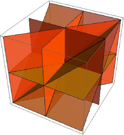
Figure 1. A picture of $\mathbb{R}^{V_{0}}_{sing}(K_{4}).$

  

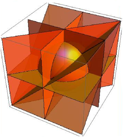
Figure 2. (Spherical) blowup of the origin in $\mathbb{R}^{V_{0}}_{sing}(K_{4}),$ where projective spaces are replaced by spheres. The maximal wonderful model would proceed by blowing up all strict transforms of lines incident to the exceptional divisor, and finally the strict transforms of the planes.

  

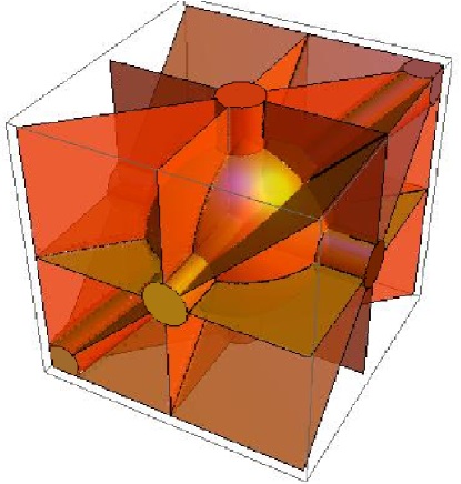
Figure 3. Minimal (spherical) model of $\mathbb{R}^{V_{0}}_{sing}(K_{4}),$ corresponding to the Fulton-MacPherson compactification of the configuration space of 4 points in $\mathbb{R}.$ After the central blowup, only those strict transforms of lines are blown up which are not a normal crossing intersection in the first place.

Remarks. In the case of the complete graph $K_{n},$ the minimal wonderful model $Y_{\mathcal{F}(\mathcal{C}_{sing}(K_{n}))}$ is known as the Fulton-MacPherson compactification [FM], while the maximal wonderful model $Y_{\mathcal{C}_{sing}(K_{n})}$ has been described in detail by Ulyanov [Ulyanov]. For any graph, the benefit of the minimal model is that the divisor is small in the sense that it has only a minimal number of irreducible components, whereas the actual construction by a sequence of blowups is less canonical. On the other hand, for the maximal model, which has a larger number of irreducible components, one can proceed in the obvious way blowing up the center and then strict transforms by increasing dimension. See figures 1, 2, 3 for an example where $M$ is supposed one-dimensional in order to be able to draw a picture. Also the resolution of projective hyperplane arrangements described in [ESV] and referred to in [BEK, Lemma 5.1] proceeds by increasing dimension but corresponds to the minimal wonderful model nonetheless. This is a special effect due to the fact that the strict transforms of hyperplanes, having codimension 1, do not need to be blown up. If the subspaces in the arrangement have higher codimension, the blowup sequence will be different. See [FM, Ulyanov] and [deCPro, Theorem 3.2] for details.

4.6. Examples

For the fixed vertex set $V=\{1,2,3,4\}$ we consider a series of graphs on $V$ with increasing complexity. Only some of them are relevant for renormalization.

$$\begin{array}[]{ll}\Gamma_{1}=\;\raisebox{-19.91684pt}{\epsfbox{4pts-gamma1.eps}}&\Gamma_{4}=\;\raisebox{-22.76228pt}{\epsfbox{4pts-gamma4.eps}}\\ \Gamma_{2}=\;\raisebox{-22.76228pt}{\epsfbox{4pts-gamma2.eps}}&\Gamma_{5}=\;\raisebox{-21.33955pt}{\epsfbox{4pts-gamma5.eps}}\\ \Gamma_{3}=\;\raisebox{-22.76228pt}{\epsfbox{4pts-gamma3.eps}}&\Gamma_{6}=\;\raisebox{-22.76228pt}{\epsfbox{4pts-gamma6.eps}}\end{array}$$

For these graphs, we examine the arrangements $M^{V_{0}}_{sing}$ and $M^{V_{0}}_{div},$ the irreducible subspaces and nested sets for the minimal and maximal building set, respectively. Write $A_{ij}$ for $A_{e}$ with $e$ an edge connecting the vertices $i$ and $j.$ Note that $A_{12}+A_{23}=A_{13}+A_{23}=A_{12}+A_{13}$ etc., and in the examples a choice of basis is made.

$$\mathcal{C}_{sing}(\Gamma_{1}) = \{A_{12},A_{23},A_{34},\mbox{ and sums thereof}\}$$

$$\left.\begin{array}[]{r}\mathcal{C}_{sing}(\Gamma_{2})\\ \mathcal{C}_{sing}(\Gamma_{3})\\ \mathcal{C}_{sing}(\Gamma_{4})\\ \end{array}\right\} = \{A_{12},A_{23},A_{24},A_{34},\mbox{ and sums thereof}\}$$

$$\mathcal{C}_{sing}(\Gamma_{5}) = \{A_{12},A_{13},A_{23},A_{24},A_{34},\mbox{ and sums thereof}\}$$

$$\mathcal{C}_{sing}(\Gamma_{6}) = \{A_{12},A_{13},A_{14},A_{23},A_{24},A_{34},\mbox{ and sums thereof}\}$$

The divergent arrangements are determined by the following collections of dual spaces:

$$\mathcal{C}_{div}(\Gamma_{1}) = \emptyset$$

$$\mathcal{C}_{div}(\Gamma_{2}) = \{A_{12}\}$$

$$\mathcal{C}_{div}(\Gamma_{3}) = \{A_{34},A_{23}+A_{34}\}$$

$$\mathcal{C}_{div}(\Gamma_{4}) = \{A_{12},A_{34},A_{23}+A_{34},A_{12}+A_{34},A_{12}+A_{23}+A_{34}\}$$

$$\mathcal{C}_{div}(\Gamma_{5}) = \{A_{34},A_{23}+A_{34},A_{12}+A_{23}+A_{34}\}$$

$$\mathcal{C}_{div}(\Gamma_{6}) = \{A_{12}+A_{23}+A_{34}\}$$

The irreducible singular subspace collections are

$$\mathcal{F}(\mathcal{C}_{sing}(\Gamma_{1})) = \{A_{12},A_{23},A_{34}\}$$

$$\left.\begin{array}[]{r}\mathcal{F}(\mathcal{C}_{sing}(\Gamma_{2}))\\ \mathcal{F}(\mathcal{C}_{sing}(\Gamma_{3}))\\ \mathcal{F}(\mathcal{C}_{sing}(\Gamma_{4}))\\ \end{array}\right\} = \{A_{12},A_{23},A_{24},A_{34},A_{23}+A_{34}\}$$

$$\mathcal{F}(\mathcal{C}_{sing}(\Gamma_{5})) = \{A_{12},A_{13},A_{23},A_{24},A_{34},$$

$$A_{12}+A_{13},A_{23}+A_{24},A_{12}+A_{23}+A_{34}\}$$

$$\mathcal{F}(\mathcal{C}_{sing}(\Gamma_{6})) = \{A_{12},A_{13},A_{14},A_{23},A_{24},A_{34},$$

$$A_{12}+A_{13},A_{12}+A_{14},A_{13}+A_{14},A_{23}+A_{34},$$

$$A_{12}+A_{23}+A_{34}\}$$

Remark. Note that these irreducible single subspace collections are in one-to-one correspondence with the terms generated by the core Hopf algebra [BlKr, KreimerSui] if one takes into account the multiplicities generated by a labeling of vertices. A detailed comparison is left to future work.

The irreducible divergent subspace collections are

$$\mathcal{F}(\mathcal{C}_{div}(\Gamma_{1})) = \emptyset$$

$$\mathcal{F}(\mathcal{C}_{div}(\Gamma_{2})) = \{A_{12}\}$$

$$\mathcal{F}(\mathcal{C}_{div}(\Gamma_{3})) = \{A_{34},A_{23}+A_{34}\}$$

$$\mathcal{F}(\mathcal{C}_{div}(\Gamma_{4})) = \{A_{12},A_{34},A_{23}+A_{34}\}$$

$$\mathcal{F}(\mathcal{C}_{div}(\Gamma_{5})) = \{A_{34},A_{23}+A_{34},A_{12}+A_{23}+A_{34}\}$$

$$\mathcal{F}(\mathcal{C}_{div}(\Gamma_{6})) = \{A_{12}+A_{23}+A_{34}\}$$

The maximal nested sets of the divergent collection wrt.  the minimal building set:

$$\mbox{ for }\Gamma_{1}: \emptyset$$

$$\mbox{ for }\Gamma_{2}: \{A_{12}\}$$

$$\mbox{ for }\Gamma_{3}: \{A_{23}+A_{34},A_{34}\}$$

$$\mbox{ for }\Gamma_{4}: \{A_{12},A_{23}+A_{34},A_{34}\}$$

$$\mbox{ for }\Gamma_{5}: \{A_{12}+A_{23}+A_{34},A_{23}+A_{34},A_{34}\}$$

$$\mbox{ for }\Gamma_{6}: \{A_{12}+A_{23}+A_{34}\}$$

The maximal nested sets of the divergent collection wrt.  the maximal building set:

$$\mbox{ for }\Gamma_{1}: \emptyset$$

$$\mbox{ for }\Gamma_{2}: \{A_{12}\}$$

$$\mbox{ for }\Gamma_{3}: \{A_{23}+A_{34},A_{34}\}$$

$$\mbox{ for }\Gamma_{4}: \{A_{12}+A_{23}+A_{34},A_{12}+A_{34},A_{12}\},$$

$$\{A_{12}+A_{23}+A_{34},A_{12}+A_{34},A_{34}\},$$

$$\{A_{12}+A_{23}+A_{34},A_{23}+A_{34},A_{34}\}$$

$$\mbox{ for }\Gamma_{5}: \{A_{12}+A_{23}+A_{34},A_{23}+A_{34},A_{34}\}$$

$$\mbox{ for }\Gamma_{6}: \{A_{12}+A_{23}+A_{34}\}$$

5. Laurent coefficients of the meromorphic extension

5.1. The Feynman distribution pulled back onto the wonderful model

Recall the definition (4) of the Feynman distribution $u_{\Gamma}=\prod_{i<j}u_{0}(x_{i}-x_{j})^{n_{ij}}.$ We write $\underline{u}_{\Gamma}=\Phi_{\ast}u_{\Gamma}$ where $\Phi$ is the projection along the thin diagonal defined at the end of section 2.1. It is clear from the discussion in section 2 that $\underline{u}_{\Gamma}=(i_{\Gamma}^{\oplus d})^{\ast}u_{0}^{\otimes|E(\Gamma)|}$ where defined. Let $\beta:Y_{\mathcal{P}}\rightarrow M^{V_{0}}$ be a wonderful model for the arrangement $M^{V_{0}}_{div}(\Gamma)$ or $M^{V_{0}}_{sing}(\Gamma).$ The purpose of this section is to study the regularized pullback $\beta^{\ast}\underline{\tilde{u}}_{\Gamma}^{s}$ (as a density-valued meromorphic function of $s$) of $\underline{\tilde{u}}^{s}_{\Gamma}$ onto $Y_{\mathcal{P}}\setminus\mathcal{E}.$

Theorem 5.1.

Let $\mathcal{N}$ be a $\mathcal{P}$-nested set in $\mathcal{C}_{div}(\Gamma)$ $(\mathcal{C}_{sing}(\Gamma)),$ and $\mathcal{B}=\{y^{i}_{e}:\,e\in E(t),\,i=0,\ldots,d-1\}$ an adapted basis with marked elements $y^{i_{A}}_{A},\,A\in\mathcal{N}.$ Then, in the chart $U^{\mathcal{B}}_{\mathcal{N}},$

(52) $$\beta^{\ast}\underline{u}_{\Gamma}(\{y^{i}_{e}\})=f_{\Gamma}(\{y^{i}_{e}\})\prod_{A\in\mathcal{N}}(y^{i_{A}}_{A})^{n_{A}}$$

where $f_{\Gamma}\in L^{1}_{loc}(U^{\mathcal{B}}_{\mathcal{N}})$ $(C^{\infty}(U^{\mathcal{B}}_{\mathcal{N}})),$ and $n_{A}\in-2\mathbb{N}.$ More precisely

(53) $$n_{A_{\gamma}}=(2-d)|E(\gamma_{s})|.$$

In addition, $f_{\Gamma}$ is $C^{\infty}$ in the variables $y^{i_{A}}_{A},$ $A\in\mathcal{N}.$

Note: $\gamma_{s}$ is the subgraph defined in Definition 2.1. Divergent subgraphs are saturated (Proposition 2.1). We write $f_{\Gamma}(\{y_{e}^{i}\})$ for $f_{\Gamma}(y_{e_{1}}^{0},\ldots,y_{e_{|E(t)|}}^{d-1})$ etc.

Proof. Recall from section 4.5 that the map $\beta$ is given in the chart $U^{\mathcal{B}}_{\mathcal{N}}$ by $\rho$ (see (48)):

$$\rho:\sum_{j=0}^{d-1}\sum_{e\in E(t)}y_{e}^{j}b_{e}^{j}\mapsto\sum_{j=0}^{d-1}\sum_{e\in E(t)}\prod_{y_{e}^{j}\preceq y_{e^{\prime}}^{k}}y^{k}_{e^{\prime}}b_{e}^{j}$$

where $\preceq$ is the partial order on the basis $\mathcal{B}=\{y_{e}^{j}\}$ of $(M^{V_{0}})^{\vee}$ adapted to $\mathcal{N}.$ Consequently, using (25),

(54) $$\beta^{\ast}\underline{u}_{\Gamma}(\{y_{e}^{j}\}) = u_{0}^{\otimes E(\Gamma)}i_{\Gamma}^{\oplus d}\rho(\{y_{e}^{j}\})$$

$$= \prod_{e\in E(\Gamma)}u_{0}\left(\left\{\Sigma_{e^{\prime}\leadsto e}\Pi_{y_{e^{\prime}}^{j}\preceq y_{e^{\prime\prime}}^{k}}y^{k}_{e^{\prime\prime}}\right\}_{j=0}^{d-1}\right).$$

By Proposition 4.8 (iv), each $\xi_{e}^{j}=\sum_{e^{\prime}\leadsto e}x_{e^{\prime}}^{j}=\Sigma_{e^{\prime}\leadsto e}\Pi_{y_{e^{\prime}}^{j}\preceq y_{e^{\prime\prime}}^{k}}y^{k}_{e^{\prime\prime}}$ is a product $x_{A}^{i_{A}}P_{\xi_{e}^{j}}(\{y_{j}^{i}\})$ where $A=p(\xi_{e}^{j})\in\mathcal{N}$ (Special case: $x_{A}^{i_{A}}=1$ if $p(\xi_{e}^{j})\not\in\mathcal{N}).$ As $u_{0}$ is homogeneous (2), the factor $x_{A}^{i_{A}}=\prod_{A\subseteq B\in\mathcal{N}}{y_{B}}^{i_{B}},$ can be pulled out, supplied with an exponent $2-d.$ Since $x_{A}^{i_{A}}=\prod_{A\subseteq B}{y_{B}}^{i_{B}},$ the factor $(y_{A_{\gamma}}^{i_{A_{\gamma}}})^{2-d}$ occurrs once for each $e\in E(\Gamma)$ such that $A_{e}\subseteq A_{\gamma},$ in other words for each $e\leq cc(\gamma).$ Hence (53). We finally show that the remaining factor

(55) $$f_{\Gamma}(\{y_{i}^{j}\})=\prod_{e\in E(\Gamma)}u_{0}(\{P_{\xi_{e}^{j}}(\{y_{i}^{k}\})\}_{j=0}^{d-1})$$

of $\beta^{\ast}\underline{u}_{\Gamma}$ satisfies $f_{\Gamma}\in L^{1}_{loc}(U^{\mathcal{B}}_{\mathcal{N}})$ if the divergent arrangement was resolved or $f_{\Gamma}\in C^{\infty}(U^{\mathcal{B}}_{\mathcal{N}})$ if the singular arrangement was resolved, respectively. The set $U_{\mathcal{N}}^{\mathcal{B}}$ contains by definition (see section 4.5) no point with coordinates $y_{i}^{j}$ such that for any building block $B\in\mathcal{P}$ all $P_{x}(\{y_{i}^{j}\})=0,$ $x\in B.$ In the case of $\mathcal{C}_{sing}(\Gamma),$ all $A_{e}\in\mathcal{P},$ $(e\in E(\Gamma)),$ since they are irreducible, see Proposition 4.2. On the other hand, $A_{e}$ is spanned by the $\xi_{e}^{j},$ $j=0,\ldots,d-1.$ Therefore for no $e\in E(\Gamma)$ all $d$ of the $P_{\xi_{e}^{j}}$ $(j=0,\ldots,d-1)$ in (55) vanish on $U_{\mathcal{N}}^{\mathcal{B}}.$ Hence, using (3), $f_{\Gamma}\in C^{\infty}(U_{\mathcal{N}}^{\mathcal{B}}).$ In the case of $\mathcal{C}_{div}(\Gamma),$ let $\gamma$ be divergent. By Proposition 4.3 we may assume without loss that $A_{\gamma}$ is irreducible. Therefore $A_{\gamma}\in\mathcal{P}$ as in the first case. By the same argument as above, not all the $P_{\xi_{e}^{j}}$ in the arguments of $\prod_{e\in E(\gamma)}u_{0}$ can vanish at the same time on $U_{\mathcal{N}}^{\mathcal{B}},$ whence this product is now locally integrable. In order to see that $f_{\Gamma}$ is $C^{\infty}$ in the $y_{A}^{i_{A}},$ it suffices to show that not all $d$ of the $P_{\xi_{e}^{j}}(\{y_{i}^{k}\})\rightarrow 0$ (for $j=0,\ldots,d-1)$ as the $y_{A}^{i_{A}}\rightarrow 0$ while the other coordinates are fixed. From Proposition 4.8 (iv) we know that every $P_{x}$ is linear in the $y_{A}^{i_{A}},$ if therefore all $P_{\xi_{e}^{j}}$ vanished at some $y_{A}^{i_{A}}=0$ they would have $y_{A}^{i_{A}}$ as a common factor. This contradicts Proposition 4.8 as then $p(\xi_{e})\subseteq A.$ $\Box$

In the preceding theorem, $\underline{u}_{\Gamma}$ was pulled back along $\beta$ as a distribution. The next corollary clarifies the situation for the density $\beta^{\ast}\tilde{u}_{\Gamma}=\beta^{\ast}(\underline{u}_{\Gamma}|dx|).$ We write $|dy|$ for $|dy_{e_{1}}^{0}\wedge\ldots\wedge dy_{e_{k}}^{d-1}|.$

Corollary 5.1.

Under the assumptions of Theorem 5.1,

(56) $$\beta^{\ast}\tilde{u}_{\Gamma}(\{y^{i}_{e}\})|dy|=f_{\Gamma}(\{y^{i}_{e}\})\prod_{A\in\mathcal{N}}|y^{i_{A}}_{A}|^{m_{A}}|dy|$$

where

(57) $$m_{A_{\gamma}}=2|E(\gamma_{s})|-d\dim H_{1}(\gamma_{s})-1\geq-1.$$

In the case of the divergent arrangement $\mathcal{C}_{div}(\Gamma),$ all $m_{A_{\gamma}}=-1,$ and moreover

(58) $$\beta^{\ast}\tilde{u}_{\Gamma}^{s}(\{y^{i}_{e}\})|dy|=f_{\Gamma}^{s}(\{y^{i}_{e}\})\prod_{A\in\mathcal{N}}|y^{i_{A}}_{A}|^{-d_{A}s+d_{A}-1}|dy|$$

where $d_{A}=\dim A.$

We also write $d_{\gamma}=d_{A_{\gamma}}.$

Proof. Formally,

$$|dx| = |\bigwedge_{e\in E(t),j=0\ldots,d-1}dx_{e}^{j}|=|\bigwedge d\prod_{y_{e}^{j}\preceq y_{e^{\prime}}^{k}}y_{e^{\prime}}^{k}|$$

$$= \prod_{A\in\mathcal{N}}|y_{A}^{i_{A}}|^{q_{A}}|\bigwedge dy^{j}_{e}|$$

where the $q_{A}$ are determined as follows. Since the $x_{e}^{j},$ $(j=0,\ldots,d-1)$ span $A_{e},$ the factor $y_{A_{\gamma}}^{i_{A_{\gamma}}}$ appears from all $dx_{e}^{j}$ such that $e\leq cc(\gamma),$ except one, namely $dx_{A_{\gamma}}^{i_{A_{\gamma}}}$ itself which corresponds to the marking. Since $t$ is an adapted spanning tree, the set $\{e\in E(t):e\leq cc(\gamma)\}$ defines a spanning forest of $\gamma,$ and one concludes using Proposition 2.4 that $q_{A_{\gamma}}=d_{\gamma}-1.$ Finally note that $\dim H_{1}(\gamma_{s})=|E(\gamma_{s})|-d_{\gamma}/d$ and $\Gamma$ is at most logarithmic. $\Box$

5.2. Combinatorial description of the Laurent coefficients

Let $V=V(\Gamma),$ $E=E(\Gamma)$ and $p:V\rightarrow V^{\prime}$ a map of sets which is not injective. In the dual this defines a map $p^{\vee}:\mathbb{R}^{V^{\prime}}\rightarrow\mathbb{R}^{V}$ sending $\sum_{v\in V^{\prime}}\alpha_{v^{\prime}}v^{\prime}$ to $\sum_{v\in V}\alpha_{p(v)}v.$ Let $E(\gamma)\subseteq E(\Gamma).$ Then the graph $\gamma_{p}$ with vertex set $V(\gamma_{p})=V^{\prime}$ and set of edges $E(\gamma_{p})=E(\gamma)$ such that $\delta_{\gamma_{p}}=\delta_{\gamma}\circ p^{\vee}:\mathbb{R}^{V(\gamma_{p})}\rightarrow\mathbb{R}^{E(\gamma_{p})}$ (see (15)) is called the graph $\gamma$ contracted along p.

Note: The graph contracted along $p$ may have loops. It is not necessarily a subgraph of $\Gamma$ anymore.

We assume, as in (6), a distinguished vertex $v_{0}\in V(\Gamma)$ such that $V_{0}=V(\Gamma)\setminus\{v_{0}\}.$ Let now $t$ be a spanning tree of $\Gamma$ and $s\subseteq t$ a subforest of $t.$ This defines a map $p_{t,s}:V(\Gamma)\rightarrow V(\Gamma)$ as follows: Let $v\in V(\Gamma)$ be given. Since $t$ is a spanning tree of $\Gamma,$ there is a unique path $t_{v}$ in $t$ from $v_{0}$ to $v.$ Let $p_{t,s}(v)$ be the unique vertex which is connected to $v$ by edges of $s$ only and is nearest to $v_{0}$ on the path $t_{v}.$

  

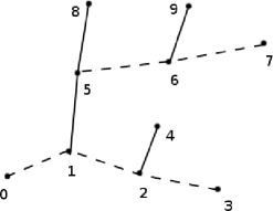
Figure 4. The edges of $s$ are broken lines, the edges of $t\setminus s$ full lines. $p_{t,s}(\{v_{0},v_{1},v_{2},v_{3}\})=v_{0},$ $p_{t,s}(v_{4})=v_{4},$ $p_{t,s}(\{v_{5},v_{6},v_{7}\})=v_{5},$ $p_{t,s}(v_{8})=v_{8},$ $p_{t,s}(v_{9})=v_{9}.$

See figure 4 for an example. This gives us a graph $\Gamma_{p_{t,s}}.$ It is obvious from the construction that $t\setminus s$ is a spanning forest of $\Gamma_{p_{t,s}}$ whereas all edges of $s$ are transformed into loops.

Let $\mathcal{N}=\{A_{\gamma_{1}},\ldots,A_{\gamma_{k}}\}$ be a $\mathcal{P}$-nested set in $\mathcal{C}_{sing}(\Gamma)$ or $\mathcal{C}_{div}(\Gamma).$ Let $t$ be an adapted spanning tree. All $\gamma_{i}$ are assumed saturated. We define the graph $\gamma_{i}//\mathcal{N}$ as follows. Let $A_{\gamma_{j_{1}}},\ldots,A_{\gamma_{j_{l}}}$ be the maximal elements $\subseteq A_{\gamma_{i}}.$ Let $s$ be the forest defined by $E(s)=E(t)\cap(E(\gamma_{j_{1}})\cup\ldots\cup E(\gamma_{j_{l}})).$ Then $\gamma_{i}//\mathcal{N}$ is the graph with edges $E(\gamma_{i})\setminus\bigcup_{m=1}^{l}E(\gamma_{j_{m}})$ contracted along the map $p_{t,s}.$

The graph $\gamma_{i}//\mathcal{N}$ obviously depends on $t,$ although only up to a permutation of the vertices, as is easily verified.

Lemma 5.1.

Under the assumptions above:

1. The graph $\gamma_{i}//\mathcal{N}$ has no loops.

2. If $\gamma_{i}$ is connected, so is $\gamma_{i}//\mathcal{N}$ (wrt.  $V_{\operatorname{eff}}(\gamma_{i}//\mathcal{N})).$

3. In the case of the divergent collection $\mathcal{C}_{div}(\Gamma),$ let $\mathcal{N}$ be a maximal nested set. If $\gamma_{i}$ is connected, $\gamma_{i}//\mathcal{N}$ is at most logarithmic and primitive. Therefore $\operatorname{res}(\gamma_{i}//\mathcal{N})$ is defined (see (43)).

4. In this case $\operatorname{res}(\gamma_{i}//\mathcal{N})$ does not depend upon the choice of an adapted spanning tree $t.$

Note that for $\mathcal{P}=\mathcal{F}(\mathcal{C})$ every $\gamma_{i}$ is connected (as it is irreducible). For non-connected $\gamma_{i},$ the statements hold for each component.

Proof. (i) Suppose $e$ were a loop in $\gamma_{i}//\mathcal{N}$ at the vertex $v.$ Since $\gamma_{i}$ has no loops, $|p_{t,s}^{-1}(v)|>1.$ However, $p_{t,s}$ moves only the vertices adjacent to edges of $s.$ We conclude $e\in E(\gamma_{j_{m}})$ as the $\gamma_{j}$ are saturated, and have a contradiction.
(ii) By construction $p^{\vee}(\sum_{v^{\prime}\in V_{\operatorname{eff}}(\gamma_{i}//\mathcal{N})}v^{\prime})=p^{\vee}(\sum_{v^{\prime}\in V(\gamma_{i}//\mathcal{N})}v^{\prime})=\sum_{v\in V(\gamma_{i})}v$ since the sum is over all vertices of $V_{\operatorname{\operatorname{eff}}}(\gamma_{i})$ (the vertices not in $V_{\operatorname{eff}}$ map to $0$). On the other hand, $p^{\vee}(x)$ of a sum $x=\sum_{v^{\prime}\in U}v^{\prime}$ where $U\subsetneq V_{\operatorname{eff}}(\gamma_{i}//\mathcal{N}),$ is not contained in $\operatorname{span}\sum_{v\in V(\gamma_{i})}v.$ Write $\delta=\delta_{\gamma_{i}}$ and $\delta_{p}=\delta_{(\gamma_{i})_{p}}.$

$$\begin{diagram}$$

Note that $\delta_{p}$ as a map into $\mathbb{R}^{E((\gamma_{i})_{p})}$ is the same as as a map into $\mathbb{R}^{E(\gamma_{i}//\mathcal{N})}$ since the missing edges are all loops. Consequently, if $x\in\ker\delta_{p},$ then $p^{\vee}(x)\in\ker\delta,$ by definition of $(\gamma_{i})_{p}.$ However, because $\gamma_{i}$ is connected, $\ker\delta=\operatorname{span}\sum_{v\in V(\gamma_{i})}v.$ Therefore $\dim\ker\delta_{p}=1,$ if $\delta_{p}$ is restricted to $V_{\operatorname{eff}}(\gamma_{i}//\mathcal{N}),$ and hence $\gamma_{i}//\mathcal{N}$ connected.
(iii) By definition, a graph $\gamma$ on $V(\Gamma)$ is divergent if and only if $\dim A_{\gamma}=(d-2)|E(\gamma)|.$ It is convergent if $\dim A_{\gamma}>(d-2)|E(\gamma)|.$ We may restrict ourselves to saturated subgraphs because the number of edges increases the susceptibility to divergences, and every divergent graph is saturated. Let $\gamma_{p}\subseteq\gamma_{i}//\mathcal{N}$ be saturated as a subgraph of $\gamma_{i}//\mathcal{N}.$ Therefore $E(\gamma_{p})\subseteq E(\gamma_{i})\setminus\bigcup_{m=1}^{l}E(\gamma_{j_{m}}).$ Let now $\gamma_{s}$ be the saturated graph for $\gamma_{p}$ as a subgraph of $\gamma_{i}.$ Since $p$ maps each component of $\gamma_{j_{m}}$ to a single vertex, $\gamma_{i}//\mathcal{N}$ has $\sum_{m=1}^{l}\dim A_{\gamma_{j_{m}}}$ components more than $\gamma_{i}.$ More generally,

$$\dim A_{\gamma_{p}}=\dim A_{\gamma_{s}}-\dim A_{s\cap\gamma_{s}}.$$

On the other hand,

$$|E(\gamma_{p})|=|E(\gamma_{s})|-|E((s\cap\gamma_{s})_{s})|.$$

Therefore $(d-2)|E(\gamma_{p})|\leq\dim A_{\gamma_{p}},$ and equality only if $\gamma_{s}=\gamma_{i}$ (equivalently $\gamma_{p}=\gamma_{i}//\mathcal{N})$ by the maximality of $\mathcal{N}.$ It follows that $\gamma_{i}//\mathcal{N}$ is divergent, and proper subgraphs $\gamma_{p}$ of $\gamma_{i}//\mathcal{N}$ are convergent, divergent, worse than logarithmically divergent if and only if they are as subgraphs of $\gamma_{i};$ whence $\gamma_{i}//\mathcal{N}$ is also at most logarithmic and primitive.
(iv) Let $t,t^{\prime}$ be two choices of an adapted spanning tree. Then $t\setminus s$ and $t^{\prime}\setminus s^{\prime}$ are spanning trees of $\gamma_{i}//\mathcal{N},$ and by the argument in the proof of Theorem 3.1 (ii) $\operatorname{res}\gamma_{i}//\mathcal{N}$ is independent of the basis chosen. $\Box$

We will shortly use this lemma in connection with the following theorem, which helps understand the geometry of the divisor $\mathcal{E}$ in $Y_{\mathcal{P}}.$

Theorem 5.2.

(see [deCPro, Theorem 3.2]) Let $\beta:Y_{\mathcal{P}}\rightarrow V$ be a wonderful model.

1. The divisor is $\mathcal{E}=\bigcup_{A\in\mathcal{P}}\mathcal{E}_{A}$ with $\mathcal{E}_{A}$ smooth irreducible and $\beta(\mathcal{E}_{A})=A^{\perp}.$

2. The components $\mathcal{E}_{A_{1}},\ldots,\mathcal{E}_{A_{k}}$ have nonempty intersection if and only if the set $\{A_{1},\ldots,A_{k}\}$ is $\mathcal{P}$-nested. In this case the intersection is transversal.

$\Box$

We also write $\mathcal{E}_{\gamma}$ for $\mathcal{E}_{A_{\gamma}}.$

We consider only the divergent case $\mathcal{C}_{div}(\Gamma)$ with arbitrary building set $\mathcal{P}$ and conclude for the Laurent expansion at $s=1:$

Theorem 5.3.

Let $\tilde{w}_{\Gamma}^{s}=\beta^{\ast}\tilde{u}_{\Gamma}^{s}$ as a density.

1. The density $\tilde{w}_{\Gamma}^{s}$ has a pole of order $N_{max}$ at $s=1,$ where $N_{max}$ is the cardinality of the largest nested set.

2. Let

   (59) $$\tilde{w}_{\Gamma}^{s}=\sum_{k=-N_{max}}^{\infty}\tilde{a}_{\Gamma,k}(s-1)^{k}.$$

   Then, for $k\leq-1,$

   $$\operatorname{supp}\tilde{a}_{\Gamma,k}=\bigcup_{|\mathcal{N}|=-k}\bigcap_{A_{\gamma}\in\mathcal{N}}\mathcal{E}_{\gamma},$$

   which is a subset of codimension $-k$. The union is over $\mathcal{P}$-nested sets $\mathcal{N}.$

3. Let $\mathcal{P}=\mathcal{F}(\mathcal{C}_{div}(\Gamma)).$ Recall that $\underline{1}$ denotes the constant function 1. Then

   (60) $$\tilde{a}_{\Gamma,-N_{max}}[\underline{1}]=\sum_{|\mathcal{N}|=N_{max}}\prod_{A_{\gamma}\in\mathcal{N}}\operatorname{res}(\gamma//\mathcal{N}).$$

   where all $\gamma$ are assumed saturated.

Recall from Theorem 5.1 that $f_{\Gamma}$ is $C^{\infty}$ in the $y_{A}^{i_{A}}.$ Therefore the canonical regularization can be used consistently (see (35)). The identity (60) is known as a consequence of the scattering formula in [CK3] in a momentum space context. More general identities for the higher coefficients can be obtained but are not necessary for the purpose of this paper.

Proof. (i) From (58), $\tilde{w}_{\Gamma}^{s}|dy|=f_{\Gamma}^{s}\prod_{A\in\mathcal{N}}|y_{A}^{i_{A}}|^{(d_{A}-1)-d_{A}s}|dy|$ in local coordinates. By the results of section 3.3, in particular (38),

(61) $$\tilde{w}_{\Gamma}^{s}|dy|=f_{\Gamma}^{s}\prod_{A\in\mathcal{N}}\left(-\frac{2\delta_{0}(y_{A}^{i_{A}})}{d_{A}(s-1)}+|y^{i_{A}}_{A}|_{fin}^{(d_{A}-1)-d_{A}s}\right)|dy|,$$

whence the first statement.
(ii) This follows from (61), using that $\mathcal{E}_{\gamma}$ is locally given by $y_{A_{\gamma}}^{i_{A_{\gamma}}}=0.$ Theorem 5.2 (ii) shows that the codimension is $k.$
(iii) Throughout this proof we assume all $\gamma$ defining the nested set are saturated. By Theorem 5.2 (ii), for $|\mathcal{N}|=N_{max},$ the set $\cap_{\gamma\in\mathcal{N}}\mathcal{E}_{\gamma}$ intersects no other $\mathcal{E}_{\gamma^{\prime}},$ $\gamma^{\prime}\not\in\mathcal{N}.$ Using (ii), $\tilde{a}_{\Gamma,-N_{max}}$ is in fact supported on a disjoint union subsets of codimension $N_{max},$ and we may compute $\tilde{a}_{\Gamma,-N_{max}}[\underline{1}]$ on each of them and sum the results up. It suffices, therefore, to show

(62) $$(-2)^{N_{max}}\int f_{\Gamma}\prod_{A_{\gamma}\in\mathcal{N}}\delta_{0}(y_{A_{\gamma}}^{i_{A_{\gamma}}})/d_{\gamma}|dy|=\prod_{A_{\gamma}\in\mathcal{N}}\operatorname{res}(\gamma//\mathcal{N})\quad\mbox{ (in }U_{\mathcal{N}}^{\mathcal{B}})$$

for all maximal nested sets $\mathcal{N}.$ Integration inside one chart suffices since there is no other nested set $\mathcal{N^{\prime}}$ such that $j(U_{\mathcal{N^{\prime}}})$ covers $\cap_{A_{\gamma}\in\mathcal{N}}\mathcal{E}_{\gamma}$ and charts from another choice of marked basis need not be considered, see the argument in the proof of Theorem 3.1 (ii). Recall (25) on $M^{V_{0}}$ and (54)

$$w_{\Gamma}(\{y_{e}^{j}\})=(\beta^{\ast}\underline{u}_{\Gamma})(\{y_{e}^{j}\})=\prod_{e\in E(\Gamma)}u_{0}(\{\sum_{e^{\prime}\leadsto e}\prod_{y_{e^{\prime}}^{j}\preceq y_{e^{\prime\prime}}^{k}}y^{k}_{e^{\prime\prime}}\}_{j=0}^{d-1}).$$

in $U_{\mathcal{N}}^{\mathcal{B}}.$ In order to study $f_{\Gamma}|_{y_{A_{\gamma}}^{i_{A_{\gamma}}}=0}$ one observes that all products $\prod_{y_{e^{\prime}}^{j}\preceq y_{e^{\prime\prime}}^{k}}y^{k}_{e^{\prime\prime}}$ vanish at $y_{A_{\gamma}}^{i_{A_{\gamma}}}=0,$ once $e^{\prime}\in E(\gamma).$ If all $d$ components $x^{0}_{e^{\prime}},\ldots,x^{d-1}_{e^{\prime}}$ of all $e^{\prime}\leadsto e$ vanish at the same time, this does not affect $f_{\Gamma},$ as it is taken care of by a power of $y_{A}^{i_{A}}$ pulled out of $u_{\Gamma}$ in (52). Consequently, for a fixed $e\in E(\Gamma),$

$$u_{0}(\{\sum_{e^{\prime}:e^{\prime}\leadsto e}\prod_{y_{e^{\prime}}^{j}\preceq y_{e^{\prime\prime}}^{k}}y^{k}_{e^{\prime\prime}}\}^{d-1}_{j=0})\prod_{A_{\gamma}\in\mathcal{N},e\in E(\gamma)}(y_{A_{\gamma}}^{i_{A_{\gamma}}})^{d-2}\prod_{A_{\gamma}\in\mathcal{N}}\delta_{0}(y_{A_{\gamma}}^{i_{A_{\gamma}}})$$

$$=u_{0}(\{\sum_{\genfrac{}{}{0.0pt}{}{e^{\prime}:e^{\prime}\leadsto e\operatorname{and}\,\forall A_{\gamma}\in\mathcal{N}}{e^{\prime}\in E(\gamma)\Rightarrow e\in E(\gamma)}}\prod_{y_{e^{\prime}}^{j}\preceq y_{e^{\prime\prime}}^{k}}y^{k}_{e^{\prime\prime}}\}_{j=0}^{d-1})\prod_{A_{\gamma}\in\mathcal{N},e\in E(\gamma)}(y_{A_{\gamma}}^{i_{A_{\gamma}}})^{d-2}.$$

On the other hand, consider the graph $\gamma//\mathcal{N}$ where $\gamma\in\mathcal{N}.$ Write $p=p_{t_{\gamma},s_{\gamma}}$ where $E(t_{\gamma})=E(t)\cap E(\gamma),$ $t$ is the chosen adapted spanning tree for $\Gamma$ and $s_{\gamma}$ the subforest defined by the maximal elements of the nested set contained in $\gamma.$ Since $\gamma$ is connected, $t_{\gamma}$ is a spanning tree of $\gamma.$ A vertex $v_{0,\gamma}\in V_{\operatorname{eff}}(t_{\gamma})$ is chosen. For each component $c$ of $s_{\gamma}$ there is a unique element $v_{c}\in V_{\operatorname{eff}}(c)$ which is nearest to $v_{0,\gamma}$ in $t_{\gamma}.$ By definition,

$$p^{\vee}(v)=\left\{\begin{array}[]{ll}\sum_{v^{\prime}\in V_{\operatorname{eff}}(c)}v^{\prime}&\mbox{ if }v=v_{c},\\ 0&\mbox{ if }v\in V_{\operatorname{eff}}(s_{\gamma})\setminus\bigcup\{v_{c}\},\\ v&\mbox{ if }v\in V(\Gamma)\setminus V_{\operatorname{eff}}(s_{\gamma}).\end{array}\right.$$

Let $x=\sum_{e\in E(t_{\gamma})}x_{e}b_{e}$ with $b_{e}=(-1)^{Q_{e}}\sum_{v\in V_{1}}v$ as in Proposition 2.7. One finds $p^{\vee}(b_{e})=(-1)^{Q_{e}}\sum_{v\in V_{1}\setminus V_{1}\cap V_{\operatorname{eff}}(c)}v$ where $c$ is the component of $s_{\gamma}$ which contains $e,$ and $c=\emptyset$ if $e\in E(t_{\gamma}\setminus s_{\gamma}).$ In particular $p^{\vee}(b_{e})=b_{e}$ if $e\in E(t_{\gamma}\setminus s_{\gamma}).$ Consequently

$$i_{\gamma//\mathcal{N}}(x) = \delta p^{\vee}(x)$$

$$= \sum_{e\in E(\gamma//\mathcal{N})}\sum_{e^{\prime}\in E(t_{\gamma})}(-1)^{Q_{e^{\prime}}}x_{e^{\prime}}\sum_{v\in V_{1}\setminus V_{1}\cap V_{\operatorname{eff}}(c)}(v:e)e$$

$$= \sum_{e\in E(\gamma//\mathcal{N})}\sum_{\genfrac{}{}{0.0pt}{}{e^{\prime}\leadsto e}{e^{\prime}\in E(t_{\gamma}\setminus s_{\gamma})}}x_{e^{\prime}}e$$

where $t_{\gamma}\setminus s_{\gamma}$ is a spanning tree for $\gamma//\mathcal{N}.$ Therefore

$$\tilde{a}_{\gamma//\mathcal{N},-1} = \prod_{e\in E(\gamma//\mathcal{N})}u_{0}(\{\sum_{\genfrac{}{}{0.0pt}{}{e^{\prime}\leadsto e}{e^{\prime}\in E(t_{\gamma}\setminus s_{\gamma})}}\prod_{y_{e^{\prime}}^{j}\preceq y_{e^{\prime\prime}}^{k}}y^{k}_{e^{\prime\prime}}\})$$

$$\times\prod_{\gamma\subseteq\gamma^{\prime}\in\mathcal{N}}(y_{A_{\gamma^{\prime}}}^{i_{A_{\gamma^{\prime}}}})^{(d-2)|E(\gamma//\mathcal{N})|}|dy|.$$

In a final step, define for each $e\in E(\Gamma)$ the minimal element $A_{\gamma_{e}}\in\mathcal{N}$ such that $e\in E(\gamma_{e}).$ We have $E(\Gamma)=\bigsqcup_{A_{\gamma}\in\mathcal{N}}\{e\in E(\Gamma):\gamma_{e}=\gamma\}$ $=\bigsqcup_{A_{\gamma}\in\mathcal{N}}E(\gamma//\mathcal{N})$ as is shown by a simple induction. Similarly $E(t)=\bigsqcup_{A_{\gamma}\in\mathcal{N}}\{e\in E(t):\gamma_{e}=\gamma\}$ $=\bigsqcup_{A_{\gamma}\in\mathcal{N}}E(t_{\gamma})\setminus E(s_{\gamma})$ is a decomposition into spanning trees since $t$ is adapted. Write $|dy|=|\bigwedge_{\genfrac{}{}{0.0pt}{}{e\in E(t)}{j=0,\ldots,d-1}}dy_{e}^{j}|$ and $|d\hat{y}|=|\bigwedge_{\genfrac{}{}{0.0pt}{}{e\in E(t),j=0,\ldots,d-1}{y_{e}^{j}\neq y_{A}^{i_{A}}}}dy_{e}^{j}|.$ Then, in $U^{\mathcal{B}}_{\mathcal{N}},$

$$\tilde{a}_{\Gamma,-N_{max}} = \tilde{w}_{\Gamma}(\{y_{e}^{j}\})\prod_{A_{\gamma}\in\mathcal{N}}|y_{A_{\gamma}}^{i_{A_{\gamma}}}|\delta_{0}(y_{A_{\gamma}}^{i_{A_{\gamma}}})|dy|$$

$$= \prod_{e\in E(\Gamma)}u_{0}(\{\sum_{\genfrac{}{}{0.0pt}{}{e^{\prime}:e^{\prime}\leadsto e\operatorname{and}\,\forall A_{\gamma}\in\mathcal{N}}{e^{\prime}\in E(\gamma)\Rightarrow e\in E(\gamma)}}\prod_{y_{e^{\prime}}^{j}\preceq y_{e^{\prime\prime}}^{k}}y^{k}_{e^{\prime\prime}}\})\prod_{\genfrac{}{}{0.0pt}{}{A_{\gamma}\in\mathcal{N}}{e\in E(\gamma)}}(y_{A_{\gamma}}^{i_{A_{\gamma}}})^{d-2}|d\hat{y}|$$

$$= \prod_{A_{\gamma}\in\mathcal{N}}(y_{A_{\gamma}}^{i_{A_{\gamma}}})^{(d-2)|E(\gamma)|}\prod_{\genfrac{}{}{0.0pt}{}{e\in E(\Gamma)}{\gamma_{e}=\gamma}}u_{0}(\{\sum_{\genfrac{}{}{0.0pt}{}{e^{\prime}\leadsto e}{\gamma_{e^{\prime}}=\gamma_{e}}}\prod_{y_{e^{\prime}}^{j}\preceq y_{e^{\prime\prime}}^{k}}y^{k}_{e^{\prime\prime}}\}_{j=0}^{d-1})|d\hat{y}|$$

$$= \bigotimes_{A_{\gamma}\in\mathcal{N}}\tilde{a}_{\gamma//\mathcal{N},-1}$$

Consequently (5.2) integrates to the product of residues as claimed. $\Box$

Theorem 5.2 and Theorem 5.3 (ii) implicitly describe a stratification of $Y_{\mathcal{P}}.$ In the next section we will show that all the information relevant for renormalization is encoded in the geometry of $Y_{\mathcal{P}}.$

6. Renormalization on the wonderful model

In this section we describe a map that transforms $\tilde{w}_{\Gamma}^{s}=\beta^{\ast}\tilde{u}_{\Gamma}^{s}$ into a renormalized distribution density $\tilde{w}_{\Gamma,R}^{s},$ holomorphic at $s=1,$ such that $\tilde{u}_{\Gamma,R}=\beta_{\ast}\tilde{w}_{\Gamma,R}^{s}|_{s=1}$ is an extension of $u_{\Gamma}$ onto all of $M^{V_{0}}$ and satisfies the following (equivalent) physical requirements:

1. The terms subtracted from $u_{\Gamma}$ in order to get $u_{\Gamma,R}$ can be rewritten as counterterms in a renormalized local Lagrangian.

2. The $u_{\Gamma,R}$ satisfy the Epstein-Glaser recursion (renormalized equations of motion, Dyson-Schwinger equations).

One might be tempted to simply define $u_{\Gamma,R}$ by discarding the pole part in the Laurent expansion of $u_{\Gamma,R}^{s}$ at $s=1.$ However, unless $\Gamma$ is primitive, this would not provide an extension satisfying those requirements, and the resulting ”counterterms” would violate the locality principle. See [Collins, Section 5.2] for a simple example in momentum space. In order to get an extension using local counterterms, one has to take into account the geometry of $Y_{\mathcal{P}}.$

The equivalence between (i) and (ii) is adressed in the original work of Epstein and Glaser [EG], see also [BS, PS, BF]. We circumvent a number of technical issues by restricting ourselves to logarithmic divergences of massless graphs on Euclidean space-time throughout the paper.

6.1. Conditions for physical extensions

In this section we suppose as given the unrenormalized distributions $\underline{u}_{\Gamma}\in\mathcal{D^{\prime}}(M^{V_{0}}\setminus M^{V_{0}}_{div}(\Gamma)),$ and examine what the physical condition (ii) implies for the renormalized distribution $\underline{u}_{\Gamma,R}\in\mathcal{D^{\prime}}(M^{V_{0}})$ to be constructed.

Let $V=\{1,\ldots,n\}$ be the vertex set of all graphs under consideration. The degree of a vertex is the number of adjacent edges. In the previous sections, $\Gamma$ was always supposed to be connected. Here we need disconnected graphs and sums of graphs. Therefore all graphs are supposed to be subgraphs of the $N$-fold complete graph $K^{N}_{n}$ on $n$ vertices with $N$ edges between each pair of vertices. $N$ can always be chosen large enough as to accomodate any graph, in a finite collection of graphs $\Gamma$ on $V,$ as one of its subgraphs.

We write $l_{V}=(l_{1},\ldots,l_{n})$ for an $\mathbb{N}_{0}$- multiindex satisfying $\sum l_{i}\in 2\mathbb{N}_{0}.$ Also $l_{V}-k_{V}=(l_{1}-k_{1},\ldots,l_{n}-k_{n}),$ ${l_{V}\choose k_{V}}={l_{1}\choose k_{1}}\ldots{l_{n}\choose k_{n}}$ etc. Let $V=I\sqcup J.$ Let $\operatorname{Bip}(k_{I},k_{J})$ be the set of $(I,J)$-bipartite graphs on $V,$ where the degree of the vertex $i$ is given by $k_{i}.$ Finally, let $(p_{I,J})_{\emptyset\subsetneq I\subsetneq V}$ be a partition of unity subordinate to the open cover $\bigcup_{\emptyset\subsetneq I\subsetneq V}C_{I}$ of $M^{V_{0}}\setminus\{0\}$ with

$$C_{I}=M^{V_{0}}\setminus M^{V_{0}}_{sing}(K_{I,V\setminus I})$$

where $K_{I,J}$ is the complete $(I,J)$-bipartite graph (i. e.  the graph with exactly one edge between each $i\in I$ and each $j\in J$). The set $M^{V_{0}}_{sing}(K_{I,J})$ is therefore the locus where at least one $x_{i}-x_{j}=0$ for $i\in I,$ $j\in J.$

The Epstein-Glaser recursion for vacuum expectation values of time-ordered products (see [BF, Equation (31)]) is given, in a euclidean version, by the equality

(64) $$t^{l_{V}}_{V}=\sum_{V=I\sqcup J}\Phi^{\ast}p_{I,J}\sum_{\genfrac{}{}{0.0pt}{}{k_{V}=0}{\sum_{i\in I}l_{i}-k_{i}=\sum_{j\in J}l_{j}-v_{j}}}^{l_{V}}{l_{V}\choose k_{V}}t^{k_{I}}_{I}t^{k_{J}}_{J}\sum_{\Gamma\in\operatorname{Bip}(l_{I}-k_{I},l_{J}-k_{J})}u_{\Gamma}$$

on $M^{V}\setminus\Delta=\Phi^{-1}(M^{V_{0}}\setminus\{0\}).$ The distributions $t^{l_{V}}_{V}$ therein, vaccuum expectation values of time-ordered Wick products, relate to the single graph distributions $u_{\Gamma}$ and their renormalizations $u_{\Gamma,R}$ as follows:

$$t_{V}^{l_{V}} = \sum_{\Gamma\in\operatorname{Gr}(l_{V})}c_{\Gamma}u_{\Gamma}\quad\mbox{ on }\Phi^{-1}(M^{V_{0}}\setminus M^{V_{0}}_{sing}(K_{n}))$$

(65) $$t_{V}^{l_{V}} = \sum_{\Gamma\in\operatorname{Gr}(l_{V})}c_{\Gamma}u_{\Gamma,R}\quad\mbox{ on }M^{V}$$

$\operatorname{Gr}(l_{V})$ is the set of all graphs $\Gamma$ with given vertex set $V(\Gamma)$ such that the degree of the vertex $i$ is $l_{i}.$ There are no external edges and no loops (edges connecting to the same vertex at both ends). The combinatorial constants $c_{\Gamma}=\frac{\prod_{i=1}^{n}l_{i}!}{\prod_{i<j}l_{ij}!}$ where $l_{ij}$ is the number of edges between $i$ and $j,$ are not needed in the following. See [Keller, Appendix B] for the complete argument.

Proposition 6.1.

On the level of single graphs, a sufficient condition for equation (64) to hold is, for any $\Gamma,$

(66) $$u_{\Gamma,R}=u_{\gamma_{1},R}\cdot u_{\gamma_{2},R}\cdot u_{\Gamma\setminus(\gamma_{1}\sqcup\gamma_{2})}\mbox{ on }\Phi^{-1}(M^{V_{0}}\setminus M^{V_{0}}_{sing}(\Gamma\setminus(\gamma_{1}\sqcup\gamma_{2})))$$

whenever $\gamma_{1},\gamma_{2}$ are connected saturated subgraphs of $\Gamma,$ such that $V_{\operatorname{eff}}(\gamma_{1})\cap V_{\operatorname{eff}}(\gamma_{2})=\emptyset.$

Note that $u_{\gamma_{1},R}\cdot u_{\gamma_{2},R}$ is in fact a tensor product since $cc(\gamma_{1})\cap cc(\gamma_{2})=0.$ The locus where the remaining factor $u_{\Gamma\setminus(\gamma_{1}\sqcup\gamma_{2})}$ is not $C^{\infty}$ is excluded by restriction to $M^{V_{0}}\setminus M^{V_{0}}_{sing}(\Gamma\setminus(\gamma_{1}\sqcup\gamma_{2})).$ The product is therefore well-defined. Note also that (66) trivially holds on $M^{V_{0}}\setminus M^{V_{0}}_{div}(\Gamma)$ by the very definition (4) of $u_{\Gamma}.$ Proposition 6.1 implies, in particular, that if $\Gamma$ is a disjoint union ($\Gamma=\gamma_{1}\sqcup\gamma_{2}$ and $V_{\operatorname{eff}}(\gamma_{1})\cap V_{\operatorname{eff}}(\gamma_{2})=\emptyset),$ then $u_{\Gamma,R}=u_{\gamma_{1},R}\otimes u_{\gamma_{2},R}$ everywhere.

The system of equations (66) is called the Epstein-Glaser recursion for $u_{\Gamma,R}.$ Recursive equations of this kind are also referred to as renormalized Dyson-Schwinger equations (equations of motion) in a momentum space context [Kreimer2, BK2].

Proof of Proposition 6.1. Let all $u_{\Gamma,R}$ satisfy the requirement of (66). We only need the case where $\{I,J\}$ with $I=V_{\operatorname{eff}}(\gamma_{1}),$ $J=V_{\operatorname{eff}}(\gamma_{2})$ is a partition, i. e.  $I\sqcup J=V.$ Since $M^{V_{0}}_{sing}(\Gamma\setminus(\gamma_{1}\sqcup\gamma_{2}))\subseteq M^{V_{0}}_{sing}(K_{I,J}),$ (66) is valid in particular on $C_{I}\supseteq\operatorname{supp}p_{I,J}.$ Furthermore, since $\gamma_{1}$ and $\gamma_{2}$ are saturated, $\Gamma\setminus(\gamma_{1}\sqcup\gamma_{2})$ is $(I,J)$-bipartite. Therefore, $t_{V}^{l_{V}}$ as in (6.1) with (66) inserted, provides one of the terms on the right hand side of (64). Conversely, every graph $\Gamma$ with prescribed vertex degrees can be obtained by chosing a partition $I\sqcup J=V,$ taking the saturated subgraphs $\gamma_{i}$ for $I$ and $\gamma_{j}$ for $J,$ respectively, and supplying the missing edges from the $(I,J)$-bipartite graph. $\Box$

6.2. Renormalization prescriptions

We consider the divergent arrangement $\mathcal{C}=\mathcal{C}_{div}(\Gamma)$ only, with building set $\mathcal{P}$ minimal or maximal, that is $\mathcal{P}=\mathcal{F}(\mathcal{C})$ or $\mathcal{C}.$ Let $\mathcal{N}$ be a nested set which, together with an adapted spanning tree $t$ and a marking of the corresponding basis $\mathcal{B},$ provides for a chart $U_{\mathcal{N}}^{\mathcal{B}}$ for $Y_{\mathcal{P}}.$

By Theorem 5.3 (ii) the subset of codimension 1 where $\tilde{w}_{\Gamma}^{s}$ has only a simple pole at $s=1$ is covered by those charts $U^{\mathcal{B}}_{\mathcal{N}}$ where $\mathcal{N}=\{A_{\gamma}\}$ with $\gamma$ any divergent (and irreducible if $\mathcal{P}=\mathcal{F}(\mathcal{C}))$ graph. From (61) one has

$$\tilde{w}_{\Gamma}^{s}|dy|=f_{\Gamma}^{s}\left(-\frac{2\delta_{0}(y_{A_{\gamma}}^{i_{A_{\gamma}}})}{d_{\gamma}(s-1)}+|y^{i_{A_{\gamma}}}_{A_{\gamma}}|_{fin}^{(d_{\gamma}-1)-d_{\gamma}s}\right)|dy|$$

In these charts, one performs one of the following subtractions in order to get a renormalized, i. e.  extended, distribution. In the first case, only the pole is removed

(67) $$\tilde{w}_{\Gamma}^{s}|dy|\mapsto\tilde{w}_{\Gamma,R_{0}}^{s}|dy|=f_{\Gamma}^{s}|y^{i_{A_{\gamma}}}_{A_{\gamma}}|_{fin}^{d_{\gamma}s-(d_{\gamma}-1)}|dy|$$

One might call this local minimal subtraction. Other extensions differ from this one by a distribution supported on $\mathcal{E}_{\gamma}.$ Here is an example of another renormalization prescription, producing a different extension:

For each $A_{\gamma}\in\mathcal{N}$ let $A_{\gamma_{1}},\ldots,A_{\gamma_{k}}\in\mathcal{N}$ be the maximal elements contained in $A_{\gamma}$ (where all graphs are assumed saturated). Choose a $\nu_{A_{\gamma}}\in C^{\infty}(Y_{\mathcal{P}})$ such that $\nu_{A_{\gamma}}|_{y_{A_{\gamma}}^{i_{A_{\gamma}}}=0}=1$ and $\nu_{A_{\gamma}}$ depends only on the coordinates $y_{e}^{j},$ $e\in E(t)\cap(E(\gamma)\setminus E(\cup_{j=1}^{k}\gamma_{j}))$ in $U_{\mathcal{B}}^{\mathcal{N}},$ and has compact support in the associated linear coordinates $x_{e}^{j},$ $e\in E(t)\cap(E(\gamma)\setminus E(\cup_{j=1}^{k}\gamma_{j})).$ The $\nu_{A_{\gamma}}$ are called renormalization conditions. In practice, the $\nu_{A_{\gamma}}$ will be chosen as described at the end of section 3.4.

The second renormalization prescription is then

(68) $$\tilde{w}_{\Gamma}^{s}|dy| \mapsto \tilde{w}_{\Gamma,R_{\nu}}^{s}|dy|$$

$$=\tilde{w}_{\Gamma}^{s}-|y^{i_{A_{\gamma}}}_{A_{\gamma}}|^{d_{\gamma}s-(d_{\gamma}-1)}[\nu_{A_{\gamma}}]_{p_{A_{\gamma}}}\delta_{0}(y^{i_{A_{\gamma}}}_{A_{\gamma}})f_{\Gamma}^{s}|dy|,$$

which is called subtraction at fixed conditions. The notation $[\nu_{A}]_{p_{A}}$ means integration along the fiber of the projection

$$p_{A}:(y_{e_{1}}^{0},\ldots,y_{e_{|E(t)|}}^{d-1})\mapsto(y_{e_{1}}^{0},\ldots,\widehat{y_{A}^{i_{A}}},\ldots,y_{e_{|E(t)|}}^{d-1})$$

defined in (31). Both prescriptions provide us local expressions holomorphic at $s=1$ in all charts $U^{\mathcal{B}}_{\mathcal{N}}$ where $\mathcal{N}$ contains a single element. It remains to define them in the other charts.

In the charts $U_{\mathcal{N}}^{\mathcal{B}},$ for a general nested set $\mathcal{N},$ where

$$\tilde{w}_{\Gamma}^{s}|dy|=f_{\Gamma}^{s}\prod_{A\in\mathcal{N}}\frac{1}{|y^{i_{A}}_{A}|^{d_{A}s-(d_{A}-1)}}|dy|$$

one applies the subtraction (67) in every factor (local minimal subtraction)

(69) $$\tilde{w}_{\Gamma,R_{0}}^{s}|dy|=f_{\Gamma}^{s}\prod_{A\in\mathcal{N}}|y^{i_{A}}_{A}|_{fin}^{(d_{A}-1)-d_{A}s}|dy|.$$

Similarly, by abuse of notation, in the same chart,

(70) $$\tilde{w}_{\Gamma,R_{\nu}}^{s}|dy|=\tilde{w}_{\Gamma}^{s}\prod_{A\in\mathcal{N}}\left(1-\ldots[\nu_{A}]_{p_{A}}\delta_{0}(y_{A}^{i_{A}})\right)|dy|$$

generalizing the subtraction at fixed conditions (68). A precise notation for (70) – which disguises however the multiplicative nature of this operation – is

(71) $$\tilde{w}_{\Gamma,R_{\nu}}^{s}|dy| = \sum_{\{A_{1},\ldots,A_{k}\}\subseteq\mathcal{N}}(-1)^{k}\prod_{A\in\mathcal{N}}\frac{1}{|y^{i_{A}}_{A}|^{d_{A}s-(d_{A}-1)}}\left[\Pi_{j=1}^{k}\nu_{A_{j}}\right]_{p_{A_{1},\ldots,A_{k}}}$$

$$\times\prod_{j=1}^{k}\delta_{0}(y_{A_{j}}^{i_{A_{j}}})f_{\Gamma}^{s}|dy|$$

where $p_{A_{1},\ldots,A_{k}}$ is the projection omitting the coordinates $y_{A_{j}}^{i_{A_{j}}},$ $j=1,\ldots,k.$ Corollary 3.1 shows that there are no infrared divergences when pushing forward along $\beta.$

Note that $\tilde{w}_{\Gamma,R_{0}}^{s}|_{s=1}|dy|$ defines a density on $Y_{\mathcal{P}},$ but this is not true for general $s:$

Proposition 6.2.

The local expressions $\tilde{w}_{\Gamma,R_{0}}^{s}|_{s=1}|dy|$ given by (69) define a density on $Y_{\mathcal{P}}.$ The $\tilde{w}_{\Gamma,R_{\nu}}^{s}$ given by (70,71) define a density-valued function on $Y_{\mathcal{P}},$ holomorphic in a neighborhood of $s=1.$

Proof. Note that $\tilde{w}_{\Gamma}^{s}$ is by construction a density for all $s.$ Local minimal subtraction: The $|y_{A}^{i_{A}}|_{fin}^{-1}$ transform like $|y_{A}^{i_{A}}|^{-1}$ under transition between charts. Subtraction at fixed conditions: Each term in the sum (71) differs from $\tilde{w}_{\Gamma}^{s}$ by a number of integrations in the $y_{A_{j}}^{i_{A_{j}}}$ and a product of delta distributions in the same $y_{A_{j}}^{i_{A_{j}}}.$ Under transition between charts, the contribution to the Jacobian from the integrations cancels the one from the delta distributions. It remains to show that $\tilde{w}_{\Gamma,R_{\nu}}^{s}$ has no pole at $s=1:$ Using that $\nu_{A}|_{y_{A}^{i_{A}}=0}=1,$ we have in local coordinates

$$\tilde{w}_{\Gamma,R_{\nu}}^{s} = \sum_{\{A_{1},\ldots,A_{k}\}\subseteq\mathcal{N}}(-1)^{k}\prod_{j=1}^{k}\left(\frac{-2\delta_{0}(y_{A_{j}}^{i_{A_{j}}})}{d_{A_{j}}(s-1)}+|y_{A_{j}}^{i_{A_{j}}}|_{fin}^{d_{A_{j}}-1-d_{A_{j}}s}[\nu_{A_{j}}]_{p_{A_{j}}}\right.$$

$$\cdot\left.\delta_{0}(y_{A_{j}}^{i_{A_{j}}})\right)\prod_{A\in\mathcal{N}\setminus\{A_{1},\ldots,A_{k}\}}\left(\frac{-2\delta_{0}(y_{A}^{i_{A}})}{d_{A}(s-1)}+|y_{A}^{i_{A}}|_{fin}^{d_{A}-1-d_{A}s}\right)f_{\Gamma}^{s}.$$

Combining this to a binomial power finishes the proof. $\Box$

Theorem 6.1.

Let $\mathcal{P}=\mathcal{F}(\mathcal{C}_{div})$ for all graphs. Then both assignments

$$\Gamma \mapsto \tilde{u}_{\Gamma,R_{0}}=\beta_{\ast}\tilde{w}_{\Gamma,R_{0}}^{s}|_{s=1},$$

$$\Gamma \mapsto \tilde{u}_{\Gamma,R_{\nu}}=\beta_{\ast}\tilde{w}_{\Gamma,R_{\nu}}^{s}|_{s=1}$$

(with consistent choice of the $\nu_{A}$) satisfy the locality condition (66) for graphs.

The proof is based on the following lemmata. All building sets $\mathcal{P}$ are minimal. If $A_{\gamma}\in\mathcal{P}$ then $\gamma$ is always supposed saturated.

Lemma 6.1.

Under the assumptions of Proposition 6.1, let $A_{\gamma}\in\mathcal{P}$ and $cc(\gamma)\not\leq cc(\gamma_{1}\sqcup\gamma_{2}).$ Then

$$\mathcal{E}_{\gamma}\subseteq\beta^{-1}(M^{V_{0}}_{sing}(\Gamma\setminus(\gamma_{1}\sqcup\gamma_{2}))).$$

Proof. If $cc(\gamma)\not\leq cc(\gamma_{1}\sqcup\gamma_{2}),$ then $\gamma$ contains an edge $e\in E(\Gamma\setminus(\gamma_{1}\sqcup\gamma_{2})).$ Consequently $A_{\gamma}^{\perp}=\bigcap_{e\in E(\gamma)}A_{e}^{\perp}\subseteq\bigcup_{e\in E(\Gamma\setminus(\gamma_{1}\sqcup\gamma_{2}))}A_{e}^{\perp}=M^{V_{0}}_{sing}(\Gamma\setminus(\gamma_{1}\sqcup\gamma_{2})).$ Since $\beta^{-1}(A_{\gamma}^{\perp})\supseteq\mathcal{E}_{\gamma},$ the result follows. $\Box$

Under the assumptions of Proposition 6.1, let

$$\mathcal{G}=\{A_{\gamma}\in\mathcal{P}:cc(\gamma)\leq cc(\gamma_{1}\sqcup\gamma_{2})\}.$$

Lemma 6.2.

A subset $\mathcal{N}\subseteq\mathcal{G}$ is nested wrt.  the minimal building set if and only if $\mathcal{N}=\mathcal{N}_{1}\sqcup\mathcal{N}_{2},$ where $\mathcal{N}_{i}$ is a nested set wrt.  the minimal building set for the connected graph $\gamma_{i}$ with vertex set $V_{\operatorname{eff}}(\gamma_{i}).$

Proof. Let $\mathcal{P}(G)=\mathcal{F}(\mathcal{C}_{div}(G))$ for a graph $G.$ First, since $V_{\operatorname{eff}}(\gamma_{1})\cap V_{\operatorname{eff}}(\gamma_{2})=\emptyset,$ every connected subgraph $\gamma$ of $\gamma_{1}\sqcup\gamma_{2}$ is either contained in $\gamma_{1}$ or in $\gamma_{2}.$ Let now $\mathcal{N}\subseteq\mathcal{G}$ be nested wrt.  $\mathcal{P}(\Gamma).$ All irreducible graphs are connected. We can therefore write $\mathcal{N}=\mathcal{N}_{1}\sqcup\mathcal{N}_{2}$ where the elements of $\mathcal{N}_{i}$ are contained in $\gamma_{i}.$ Since $\gamma_{i}$ is saturated, a subgraph of $\gamma_{i}$ is irreducible as a subgraph of $\gamma_{i}$ if and only if it is as a subgraph of $\Gamma.$ Consequently the $\mathcal{N}_{i}$ are $\mathcal{P}(\gamma_{i})$-nested because $\mathcal{P}(\gamma_{i})\subseteq\mathcal{P}(\Gamma).$ Conversely, suppose $\mathcal{N}_{1}=\{A_{\gamma_{i}},i\in I\}$ and $\mathcal{N}_{2}=\{A_{\gamma_{j}},j\in J\}$ are given. Let some $\gamma_{i_{1}},\ldots,\gamma_{i_{l}}\subseteq\gamma_{1}$ and $\gamma_{j_{1}},\ldots,\gamma_{j_{m}}\subseteq\gamma_{2}$ be pairwise noncomparable. Then the sum $\sum_{k=1}^{l}A_{\gamma_{i_{k}}}+\sum_{n=1}^{m}A_{\gamma_{j_{n}}}$ is in fact a decomposition into two terms and therefore not contained in $\mathcal{P}(\Gamma),$ unless one of the two terms is zero. But in this case, the other term is a nontrivial decomposition itself, for it is not contained in $\mathcal{P}(\gamma_{i}).$ Therefore it is not contained in $\mathcal{P}(\Gamma),$ and $\mathcal{N}_{1}\sqcup\mathcal{N}_{2}$ is nested wrt.  $\mathcal{P}(\Gamma).$ $\Box$

Proof of Theorem 6.1. Let $\Gamma,\gamma_{1},\gamma_{2}$ as in Proposition 6.1. Let $\phi\in\mathcal{D}(M^{V_{0}})$ such that $\operatorname{supp}\phi\cap M^{V_{0}}_{sing}(\Gamma\setminus(\gamma_{1}\sqcup\gamma_{2}))=\emptyset.$ In a first step, we study the compact set $X=\operatorname{supp}\psi$ where $\psi=\beta^{\ast}\phi.$ By Lemma 6.1, $X$ does not intersect any $\mathcal{E}_{\gamma}$ where $\gamma\in\mathcal{P}\setminus\mathcal{G}$. Therefore

$$X\cap j^{\mathcal{B}}_{\mathcal{N}}(U_{\mathcal{N}}^{\mathcal{B}})\subseteq j^{\mathcal{B}}_{\mathcal{N}\cap\mathcal{G}}(U^{\mathcal{B}}_{\mathcal{N}\cap\mathcal{G}})$$

(where at the right hand side the marking of $\mathcal{B}$ is restricted to $\mathcal{N}\cap\mathcal{G}).$ In order to test (66), it suffices thus to consider the $U_{\mathcal{N}}^{\mathcal{B}}$ where $\mathcal{N}\in\mathcal{G}.$ Fix now such an $\mathcal{N}\in\mathcal{G}.$ In a second step, assume for simplicity that $V_{\operatorname{eff}}(\gamma_{1})=\{1,\ldots,i\},$ $V_{\operatorname{eff}}(\gamma_{2})=\{i+1,\ldots,i+j\}$ and write $V_{r}=n-(i+j)+1$ (By the remark in the proof of Proposition 6.1 we really only need the case where $V_{r}=1$). Now consider the map $\beta_{1,2}:Y_{\mathcal{P}(\gamma_{1})}\times Y_{\mathcal{P}(\gamma_{2})}\times M^{V_{r}}\rightarrow M^{V_{0}}$ which is the cartesian product of two wonderful models (with two minimal building sets) for the graphs $\gamma_{1}$ and $\gamma_{2},$ and a factor corresponding to the remaining edges of an adapted spanning tree for $\Gamma$ where a spanning tree for $\gamma_{1}$ and $\gamma_{2}$ have been removed. The map is the identity on this third factor. If $U^{\mathcal{B}_{i}}_{\mathcal{N}_{i}}$ is a chart for $Y_{\mathcal{P}(\gamma_{i})},$ then $U^{\mathcal{B}_{1}}_{\mathcal{N}_{1}}\times U^{\mathcal{B}_{2}}_{\mathcal{N}_{2}}\times M^{V_{r}}$ is a chart for the product. As the nested sets $\mathcal{N}_{1}$ and $\mathcal{N}_{2}$ and the marking $\mathcal{B}_{1}$ and $\mathcal{B}_{2}$ of the basis vary, one obtains an atlas for $Y_{\mathcal{P}(\gamma_{1})}\times Y_{\mathcal{P}(\gamma_{2})}\times M^{V_{r}}.$ Similarly, let $q^{\mathcal{B}_{1},\mathcal{B}_{2}}_{\mathcal{N}_{1},\mathcal{N}_{2}}=q^{\mathcal{B}_{1}}_{\mathcal{N}_{1}}\otimes q^{\mathcal{B}_{2}}_{\mathcal{N}_{2}}\otimes id$ be a subordinate partition of unity with compact support for the compact set $X^{\prime}=\operatorname{supp}\beta^{\ast}_{1,2}\phi$ in $Y_{\mathcal{P}(\gamma_{1})}\times Y_{\mathcal{P}(\gamma_{2})}\times M^{V_{r}}.$
In a third step, we use Lemma 6.2 to identify $\mathcal{P}(\Gamma)$-nested sets $\mathcal{N}\subseteq\mathcal{G}$ with $\mathcal{N}_{1}\sqcup\mathcal{N}_{2},$ and to show that there is a partition of unity $p_{\mathcal{N}}^{\mathcal{B}}$ for $X\subset Y_{\mathcal{P}}$ subordinate to the atlas $U^{\mathcal{B}}_{\mathcal{N}},$ which looks locally like $q^{\mathcal{B}_{1},\mathcal{B}_{2}}_{\mathcal{N}_{1},\mathcal{N}_{2}}.$ Since $U^{\mathcal{B}}_{\mathcal{N}}=U^{\mathcal{B}_{1}}_{\mathcal{N}_{1}}\times U^{\mathcal{B}_{2}}_{\mathcal{N}_{2}}\times M^{V_{r}}\setminus\cup_{A\in\mathcal{P}\setminus\mathcal{G}}Z_{A},$ (see section 4.5), with $j^{\mathcal{B}}_{\mathcal{N}}=j^{\mathcal{B}_{1}}_{\mathcal{N}_{1}}\times j^{\mathcal{B}_{2}}_{\mathcal{N}_{2}}\times id,$ the $q^{\mathcal{B}_{1},\mathcal{B}_{2}}_{\mathcal{N}_{1},\mathcal{N}_{2}}$ provide indeed such a partition of unity $p_{\mathcal{N}}^{\mathcal{B}}$ with compact support, because a small enough neighborhood of $X$ does not intersect any $Z_{A},$ $A\not\in\mathcal{G}.$
Finally in a chart $U^{\mathcal{B}}_{\mathcal{N}},$ identified with $U^{\mathcal{B}_{1}}_{\mathcal{N}_{1}}\times U^{\mathcal{B}_{2}}_{\mathcal{N}_{2}}\times M^{V_{r}},$ by definition (69,70), the renormalized distributions satisfy

$$\tilde{w}_{\Gamma,R}(y)|dy|=\tilde{w}_{\gamma_{1},R}\tilde{w}_{\gamma_{2},R}\tilde{w}_{\Gamma\setminus(\gamma_{1}\sqcup\gamma_{2})}(y)|dy|$$

where on the right hand side pullbacks along $\beta_{1,2}$ are understood. Let $\psi_{1,2}=\beta^{\ast}_{1,2}\phi.$ Since also $\beta=\beta_{1,2}$ in this chart, we have $\psi=\psi_{1,2}$ in local coordinates. This finishes the proof. $\Box$

Remarks. Local minimal subtraction is easily defined, but depends on the choice of regularization in a crucial way. The subtraction at fixed conditions is independent of the regularization and therefore the method of choice for the renormalization of amplitudes and non-perturbative computations.
If one extends the requirement (66) to general decompositions $A_{\Gamma}=A_{\gamma_{1}}\oplus A_{\gamma_{2}}$ into connected saturated subgraphs (the proof of Theorem 6.1 is easily adapted to this), then it is obvious that the minimal model $(\mathcal{P}=\mathcal{F}(\mathcal{C}_{div}(\Gamma)))$ provides exactly the right framework for renormalization. On the other hand, on the maximal model $(\mathcal{P}=\mathcal{C}_{div}(\Gamma)),$ for which Lemma 6.2 usually fails to hold, unnecessary subtractions are required if there are disjoint or, more generally, reducible divergent subgraphs. Locality must then be imposed by additional conditions. It can be shown that local renormalization schemes such as local minimal subtraction can also be applied on the maximal (and all intermediate) models, as will be reported elsewhere.

6.3. Hopf algebras of Feynman graphs

In this section we relate our previous results to the Hopf algebras introduced for renormalization by Connes and Kreimer [Kreimer, CK2], and generalized in [BlKr]. This is not entirely straightforward, see also the remarks at the end of this section. Isolating suitable polynomials in masses and space-time derivatives, position space Green functions can be chosen to have a perturbative expansion in terms of logarithmic divergent coefficients. Thus, in summary, as long as worse than logarithmic divergences are avoided, the Hopf algebras for renormalization in momentum space [BlKr] and position space are the same.

Only the divergent collection $\mathcal{C}_{div}(\Gamma)$ and the minimal building set $\mathcal{P}=\mathcal{F}(\mathcal{C}_{div}(\Gamma))$ is considered at this stage, and irreducible and nested refer to this setting.

Definition 6.1.

Two Feynman graphs $\Gamma_{1},\Gamma_{2}$ are isomorphic if there is an isomorphism between their exact sequences (15) for a suitable orientation of edges.

Lemma 6.3.

Let $\gamma\subsetneq\Gamma$ be divergent graphs where $\Gamma$ is connected and at most logarithmic. Let $t$ be an adapted spanning tree for the nested set $\mathcal{N}=\{\Gamma,\gamma\}.$ Then the isomorphism class of $\Gamma//\mathcal{N}$ is independent of $t$ and $\Gamma//\mathcal{N}$ connected, divergent and at most logarithmic.

In this case we write $\Gamma//\gamma$ for the isomorphism class of $\Gamma//\mathcal{N}.$

Proof. Follows from Lemma 5.1 (ii),(iii) and the definition of the quotient graph using $p_{t,s}.$ $\Box$

Let $\mathcal{H}_{FG}$ be the polynomial algebra over $\mathbb{Q}$ generated by the empty graph (which serves as unit) and isomorphism classes of connected, at most logarithmic, divergent graphs. There is no need to restrict to graphs of a specific interaction, but this can obviously be done by introducing external (half-) edges and fixing the degree of the vertices. All subgraphs are now understood to have vertex set $V_{\operatorname{eff}}.$ Products of linear generators of $\mathcal{H}_{FG}$ are identified with disjoint unions of graphs. One defines

(72) $$\Delta(\Gamma)=\sum_{\gamma\subseteq\Gamma}\gamma\otimes\Gamma//\gamma$$

where in the sum only divergent subgraphs $\gamma$ are understood, including the empty graph. The quotient graph $\Gamma//\gamma$ is well-defined and a generator of $\mathcal{H}_{FG}$ by Lemma 6.3. One extends $\Delta$ as an algebra homomorphism onto all of $\mathcal{H}_{FG}.$

By the analysis of [BlKr, Section 2.2], the map $\Delta:\mathcal{H}_{FG}\rightarrow\mathcal{H}_{FG}\otimes\mathcal{H}_{FG}$ is coassociative. Note that divergent and at most logarithmic implies one-particle-irreducible (core) as in [BlKr]:

Definition 6.2.

A graph $\Gamma$ is called core (one-particle irreducible) if $\dim$ $H_{1}(\Gamma\setminus e)<\dim H_{1}(\Gamma)$ for any $e\in E(\Gamma).$

Proposition 6.3.

A divergent, at most logarithmic graph $\Gamma$ is core.

Proof. If $\dim H_{1}(\Gamma\setminus e)=\dim H_{1}(\Gamma)$ for some $e\in E(\Gamma)$ then $\Gamma\setminus e$ would be worse than logarithmically divergent. $\Box$

One can divide $\mathcal{H}_{FG}$ by the ideal $\mathcal{I}$ generated by all polynomials $\gamma-\prod\gamma_{j}$ where $A_{\gamma}=A_{\gamma_{1}}\oplus\ldots\oplus A_{\gamma_{j}}$ is an irreducible decomposition, as in [BlKr, Equation (2.5)]. Indeed, if $\gamma$ is connected and $A_{\gamma}=A_{\gamma_{1}}\oplus A_{\gamma_{2}}$ a decomposition then $\gamma$ is a join: $E(\gamma)=E(\gamma_{1})\sqcup E(\gamma_{2})$ and $V_{\operatorname{eff}}(\gamma_{1})\cap V_{\operatorname{eff}}(\gamma_{2})=\{v\}.$ We refer then to [BlKr, Equation (2.5)] for the complete argument that $\mathcal{I}$ is a coideal. The quotient Hopf algebra is denoted $\overline{\mathcal{H}}_{FG}=\mathcal{H}_{FG}/\mathcal{I},$ and we will use only this Hopf algebra in the following. It corresponds to the minimal building set. The antipode is denoted $S$ and the convolution product of linear endomorphisms $f\star g=m(f\otimes g)\Delta.$ Note that a connected divergent graph $\Gamma$ is primitive in the sense of Definition 3.4 if and only if $\Delta(\Gamma)=\emptyset\otimes\Gamma+\Gamma\otimes\emptyset.$

Theorem 6.2.

If $\Gamma$ is irreducible,

$$S(\Gamma) = \sum_{A_{\Gamma}\in\mathcal{N}}(-1)^{|\mathcal{N}|}\prod_{A_{\gamma}\in\mathcal{N}}\gamma//\mathcal{N},$$

where the sum is over nested sets $\mathcal{N}$ wrt.  $\mathcal{F}(\mathcal{C}_{div}(\Gamma)).$

Proof. Since the antipode satisfies $S(\emptyset)=\emptyset$ and

$$S(\Gamma)=-\sum_{\gamma\subsetneq\Gamma}S(\gamma)\Gamma//\gamma,$$

for $\Gamma$ irreducible, $\gamma$ divergent, one has $S(\Gamma)=-\Gamma$ if $\Gamma$ is primitive. Let now $\Gamma$ be general irreducible. The sum over nested sets $\mathcal{N}$ wrt.  $\mathcal{F}(\mathcal{C}_{div}(\Gamma))$ containing $A_{\Gamma}$ can be written as a sum over proper divergent subgraphs $\gamma$ of $\Gamma$ and nested sets $\mathcal{N^{\prime}}$ wrt.  $\mathcal{F}(\mathcal{C}_{div}(\gamma))$ containing the irreducible components of $A_{\gamma}$ such that $\mathcal{N}=\mathcal{N}^{\prime}\cup\{A_{\Gamma}\}.$ By Lemma 6.3, $\Gamma//\gamma=\Gamma//\mathcal{N},$ and the statement follows by induction. $\Box$

By Theorem 5.3 (ii)-(iii), the antipode $S$ describes thus the stratification of the divisor $\mathcal{E}$ of $Y_{\mathcal{P}}.$ A similar (but weighted) sum is given by $S\star Y$ where $Y$ is the algebra homomorphism $Y:\mathcal{H}_{FG}\rightarrow\mathcal{H}_{FG},$ $Y(\Gamma)=\dim H_{1}(\Gamma)\Gamma,$ see for example [CK3]. This provides the link between the scattering formula of [CK3] and Theorem 5.3 (iii), and we refer to future work for the details.

In the case of dimensional regularization and minimal subtraction, one considers algebra homomorphisms from $\mathcal{H}_{FG}$ into an algebra of Laurent series in the regulator, and a projector onto the finite part of the series, in order to describe the renormalization process [Kreimer, CK2, CK3]. In our framework, the Hopf algebra is encoded in the geometry of the divisor. The renormalization process is simply to approach the divisor and perform the simple subtraction along the irreducible components, and to take the product of the subtracted factors where the components intersect. Therefore the renormalization schemes studied here (69)-(71) can again be described by the antipode twisted with a subtraction operator. The latter depends however on local information as opposed to global minimal subtraction. A comprehensive discussion of the difference between local renormalization schemes as described here and (global) minimal subtraction is reserved for future work.

Remarks. The role of the Connes-Kreimer Hopf algebras in Epstein-Glaser renormalization was previously discussed in [GBL], [Pinter2] and [BK]. The third paper, which is about entire amplitudes and uses rooted trees, relies on a quite symbolic notation which is now justified by the results of the previous sections. A general flaw in the first paper [GBL] is revealed in the introduction of [Pinter2]. On the other hand the coproduct in the second paper [Pinter2] does not seem to be coassociative the way it is defined. As a counterexample consider the cycle on four vertices plus two additional edges between a pair of vertices. This can be repaired by introducing irreducible, core or at most logarithmic and saturated subgraphs as it is done here. See [BlKr, Section 2.2] for a general discussion for which classes $\mathcal{P}$ of graphs the map $\Delta(\Gamma)=\sum_{\genfrac{}{}{0.0pt}{}{\gamma\subseteq\Gamma}{\gamma\in\mathcal{P}}}\gamma\otimes\Gamma//\gamma$ has a chance of being coassociative.

6.4. Amplitudes, non-logarithmic divergences and regulators

In this section we briefly sketch how to extend our previous results, which are so far confined to single graphs with at most logarithmic divergences, to a more general class of graphs. Indeed, if one considers amplitudes, or vacuum expectation values of time-ordered products in the Epstein-Glaser framework, one wants to regularize and renormalize sums of Feynman distributions simultaneously, and some of them will obviously have worse than logarithmic singularities.

For an introductory discussion of non-logarithmic divergences the reader is referred to [BlKr, Section 7.4], [Collins, Section 5]. The general philosophy is to reduce seemingly non-logarithmic (quadratic etc.) divergences to logarithmic ones by isolating contributions to different terms in the Lagrangian (such as wave function renormalization, mass renormalization); and by projecting onto a subspace of distribution-valued meromorphic functions where local terms with infrared divergences are discarded. This shall only be sketched at the example of the primitive graph

$$\Gamma=\;\raisebox{-22.76228pt}{\epsfbox{4pts-einer.eps}}\;,\quad\underline{u}_{\Gamma}(x)|d^{6}x|=\frac{|d^{6}x|}{x^{8}}$$

in $d=6$ dimensions, which is quadratically divergent. By (33), $\underline{u}^{s}_{\Gamma}$ has relevant poles at $s=\frac{3}{4}$ and $s=1.$ Indeed, by (33),

(73) $$\tilde{w}_{\Gamma}^{s}|dy|=\frac{f^{s}_{\Gamma}(y)|dy|}{|y^{0}|^{8s-5}}=-\left(\frac{\delta_{0}(y^{0})}{4s-3}+\frac{\delta^{\prime\prime}_{0}(y^{0})}{8(s-1)}-|y^{0}|^{5-8s}_{fin}\right)f^{s}_{\Gamma}(y)|dy|.$$

Note that neither the residue at $s=\frac{3}{4}$ nor $|y^{0}|^{5-8s}_{fin}f^{s}_{\Gamma}$ is globally defined as a distribution density. One would like to work in a space of distributions where $w_{\Gamma}$ is equivalent to a linear combination of distribution densities with at most logarithmic singularities, having only a pole at $s=1.$ If one disposes of an infrared regulation such that the so-called adiabatic limit vanishes

(74) $$u^{s}_{\Gamma}[\underline{1}]=0$$

one can subtract $u_{\Gamma}^{s}[\underline{1}]\delta_{0}$ from (73) without changing it:

$$\tilde{w}_{\Gamma}^{s}|dy| = w_{\Gamma}^{s}-\delta_{0}(y^{0})\int_{\mathcal{E}}\tilde{w}_{\Gamma}^{s}(z)|dz|$$

$$= -\left(\frac{\delta_{0}(y^{0})}{4s-3}+\frac{\delta^{\prime\prime}_{0}(y^{0})}{8(s-1)}-|y^{0}|^{5-8s}_{fin}\right)f^{s}_{\Gamma}(y)|dy|$$

$$-\delta_{0}(y^{0})\left(-\frac{1}{4s-3}+\mbox{holomorphic terms}\right),$$

which kills the pole at $s=\frac{3}{4}$ and leaves a linear ultraviolet divergence. Using similar subtractions of zero the linear divergence may then be reduced to logarithmic ones and convergent terms, again at the expense of introducing infrared divergent integrals which vanish however in a quotient space where $u^{s}_{\Gamma}[\underline{1}]=0$ for all $\Gamma.$ We have not worked out the general case, but dimensional regularization suggests that it can be done consistently. Indeed, the idea (74) can be traced back to the ”identity”

(75) $$\int d^{d}kk^{2\alpha}=0,\quad\alpha\mbox{ arbitrary}$$

in momentum space dimensional regularization, see also [Collins, Sections 4.2, 4.3], [BlKr, Remark 7.6]. Equation (75) is a consequence of the fact that dimensional regularization balances ultraviolet and infrared divergences, using only one regulator $d.$

A complete treatment of non-logarithmic singularities and entire amplitudes is reserved for future work, as well as a more general study of regularization methods, such as dimensional regularization, in position space. Whereas the analytic regularization used in this paper is based on raising the propagator to a complex power, dimensional regularization would replace $d$ by $d-2s,$ $s\in\mathbb{C}$ in (1). This can be seen to lead to very similar expressions, simplifying the constants in (43), (58) etc.

7. Final remarks

Pulling back the Feynman distribution onto a smooth model with normal crossing divisor seems an obvious thing to do for an algebraic geometer. Less obvious is maybe the question which kind of smooth model is useful and how renormalization depends on the choice of a model. Before addressing this question let us first point out what changes if spherical instead of projective blowups are used (as in [AS] and in the figures in section 4) – this choice is possible since we are only interested in blowing up a real locus. In a spherical blowup of a point in some $\mathbb{R}^{m},$ the exceptional locus is a codimension one sphere instead of a codimension one projective space. In order to adjust to this different situation, one simply introduces for example around equation (3.2) twice the number of charts, say $\rho_{i}^{\pm}:U_{i}^{\pm}\rightarrow\mathcal{M}\times S^{m-1},$ where now $U_{i}^{\pm}\subset U_{i}$ is the half-space $y_{i}\geq 0$ resp.  $y_{i}\leq 0,$ and replaces $[z_{1},\ldots,z_{n}]$ by $[z_{1},\ldots,z_{n}]_{+}$ which means that only an action of $\mathbb{R}_{+}$ is divided out. (In fact, the choice of sign made in (3.2) is exactly the one obtained from identifying two antipodal charts of the spherical blowup in the right way so as to have $\mathcal{E}$ oriented.) This makes the spherical blowup $Y$ a manifold with boundary.

As is well-known, the spherical De Concini-Procesi models, and in particular the spherical Fulton-MacPherson compactification [AS], are manifolds with corners since they are submanifolds of a product of manifolds with boundary (compare (44)). Equations (44), (48) etc. have to be modified accordingly. The corners are the expense to be paid in order to get orientability, and one does not seem to gain or lose much by trading one for the other. For the simple kind of propagator $u_{0}$ studied in this paper the analysis is more or less the same, taking into account that since the sphere is the double cover of the projective space, the spherical residues come with a factor 2 compared to the projective residues.

It is obvious that the Fulton-MacPherson compactification $M[n]$ (minimal De Concini-Procesi model for $M^{V_{0}}_{sing}(K_{n})$) is good for all Feynman distributions at the same time, and therefore for entire amplitudes, which are sums of Feynman distributions. The combinatorics of the nested sets for $M[n]$ resemble the Hopf algebra of rooted trees [Kreimer, Kreimer3]. We chose to work with the graph-specific models because we wanted to make the connection to the Hopf algebra of Feynman graphs and to Zimmermann’s forest formula explicit. One difference in renormalizing a Feynman graph $\Gamma$ on $M[n]$ and on the other hand on $Y_{\mathcal{F}(C_{div}(\Gamma))}$ is that in the first case (66) really holds only for disjoint unions of subgraphs $\gamma_{1},$ $\gamma_{2}$, whereas in the second case an implicit renormalization condition ”(66) also for more general decompositions (joins) $V_{\operatorname{eff}}(\gamma_{1})\cap V_{\operatorname{eff}}(\gamma_{2})=\{v\}$” is introduced. See also the corresponding remark (v) in [BlKr, 1.3]. If one does not like this condition, one can use instead a non-minimal, intermediate building set where certain reducibilities are allowed.

In the recent paper [BlKr], which studies the Schwinger parametric representation of Feynman integrals, a toric compactification of the complement of certain coordinate linear spaces is used in order to understand the renormalized Feynman distribution as a period of a limiting mixed Hodge structure. We also mention [Marcolli, BognerWeinzierl1] for recent related research in the parametric representation, [Hollands] with regard to the operator-product expansion, and [Nikolov] for cohomological aspects.

Beyond the open problems already mentioned there arise three immediate questions. The first is to find the right analytic framework in order to generalize our results to arbitrary propagators on manifolds, with a more versatile notion of regularization than the ad-hoc analytic regularization used here. The second question is how the motivic description of renormalization in [BlKr] is related to our approach. And finally it remains to carry out a general study of finite renormalization and the renormalization group in the geometric context we have introduced.