Algebraic density functionals

Abstract

A systematic strategy for the calculation of density functionals (DFs) consists in coding informations about the density and the energy into polynomials of the degrees of freedom of wave functions. DFs and Kohn-Sham potentials (KSPs) are then obtained by standard elimination procedures of such degrees of freedom between the polynomials. Numerical examples illustrate the formalism.

Existence theorems HK for DFs do not provide directly constructive algorithms. Fortunately, the Kohn-Sham (KS) method KS spares the construction of a “kinetic functional” and reduces energy and density calculations to the tuning of a local potential, $v_{KS}(r).$ Hence, a considerable amount of work has been dedicated to detailed estimates of electronic correlation energies and the corresponding KSPs, see for instance HarJon ; SolSav ; TCH . Many authors were also concerned with representability and stability questions, see for instance CCR and, for calculations in subspaces, see Har and PBLB . For cases where the mapping between potential and density shows singularities, see KAD . For reviews of the rich multiplicity of derivations of DFs and KS solutions and their properties, we refer to DG and ParYan , and, for nuclear physics, to DFP .

Local or quasi local approximations use the continuous infinity of values $\rho(\mathbf{r}),\forall\mathbf{r}$, as the parameters of the problem. However, whether for atoms, molecules or nuclei, a finite number of parameters is enough to describe physical situations. For instance, Woods-Saxon nuclear profiles notoriously make good approximations, depending only on a handful of parameters, and it is easy to add a few parameters describing, for example, long tails and/or moderate oscillations of the density. (High frequency oscillations are unlikely, for they might cost large excitation energies.) We can stress here, in particular, the one-dimensional nature of the radial density functional (RDF) theory GirRDF , valid for nuclei and/or atoms, isolated, described by rotationally-invariant Hamiltonians; the constrained density minimization of energy LevLie returns isotropic densities, with radial profiles, $\rho(r),0\leqslant r<\infty$. The number of parameters to describe a nuclear density, therefore, can be restricted to maybe $\sim 10$ at most; situations with $\sim 20$ parameters are a luxury. For molecules, shapes are much more numerous, but a finite, while large number of parameters, truncating a list of multipoles for instance, still makes a reasonable frame. Practical DFs, therefore, can boil down to functions of a finite number of parameters. Functional variations can then be replaced by simple derivatives.

This Letter shows how information about both the density and the energy can be recast into polynomials. This allows elimination of part of the parameters. Further polynomial manipulations locate energy extrema. Only density parameters are left. The same method gives KSPs. Finally we offer a discussion and conclusion.

Consider a basis of $n$ orthonormalized, single-particle states, $\varphi_{\alpha}(\mathbf{r}\sigma\tau)$, where spin and isospin labels $\sigma\tau$ will be understood. The orthonormalized Slater determinants $\phi_{i}$ made out of the $\varphi_{\alpha}$’s for $N$ fermions make a finite subspace, of some dimension $\mathcal{N},$ in which eigenstates of the physical Hamiltonian $H$ can be approximated by configuration mixings, $\Psi=\sum_{i=1}^{\mathcal{N}}(C_{i}+iC^{\prime}_{i})\phi_{i}$. Here $C_{i}$ and $C^{\prime}_{i}$ are the real and imaginary parts, respectively, of the mixing coefficients, but, in practice, with real matrix elements, $H_{ij}=\langle\phi_{i}|H|\phi_{j}\rangle$, of the Hamiltonian $H$, the imaginary parts $C^{\prime}_{i}$ vanish. Both the energy $\eta$ and the normalization are quadratic functions of such coefficients,

$$\eta=\sum_{i,j=1}^{\mathcal{N}}C_{i}H_{ij}C_{j},\text{ }\sum_{i=1}^{\mathcal{N}}C_{i}^{2}=1.$$ (1)

Let $a_{\mathbf{r}}^{\dagger}$ and $a_{\mathbf{r}}$ be the usual creation and annihilation operators at position $\mathbf{r}$. Tabulate the matrix elements $\left\langle\phi_{j}\left|a_{\mathbf{r}}^{\dagger}a_{\mathbf{r}}\right|\phi_{j}\right\rangle.$ The density corresponding to $\Psi$ is, again, quadratic with respect to the $C_{i}$’s,

$$\rho(\mathbf{r})=\sum_{ij}C_{i}\left\langle\phi_{j}\left|a_{\mathbf{r}}^{\dagger}a_{\mathbf{r}}\right|\phi_{j}\right\rangle C_{j},$$ (2)

and any parameter that is linear with respect to moments of the density is also a quadratic function of the $C_{i}$’s.

Let $\{S_{\nu}(\mathbf{r})\},\ \nu=1,\dots,\infty,$ be a complete orthonormal set of “vanishing average” functions. Namely, the two sets of conditions, $\int d\mathbf{r}\,S_{\nu}(\mathbf{r})=0,\forall\nu$, and, $\int d\mathbf{r}S_{\mu}(\mathbf{r})S_{\nu}(\mathbf{r})=\delta_{\mu\nu},\forall\mu\nu$, are satisfied. Such sets are easy to find; in the case of one-dimensional problems, including radial ones, they can be implemented by means of orthogonal polynomials Gi05 ; Nor and a generalization to more dimensions is easy. Then subtract from $\rho$ some reference density, $\rho_{0},$ obtained by some approximation relevant for the $N$ fermions. The difference, $\Delta\rho=\rho-\rho_{0}$, is of a vanishing average, since, by definition, both $\rho$ and $\rho_{0}$ integrate out to $N$. Then the Fourier coefficients,

$$\Delta_{\nu}=\int d\mathbf{r}\;S_{\nu}(\mathbf{r})\Delta\rho(\mathbf{r}),$$ (3)

define $\rho$, as $\rho=\rho_{0}+\sum_{n=1}^{\infty}\Delta_{\nu}S_{\nu}$. As already stated, this expansion of $\rho$ can be truncated. at some realistic order $\mathcal{N}^{\prime}$, lower than the number of independent parameters $C_{i}$. The $\Delta_{\nu}$’s are quadratic in the $C_{i}$’s,

$$\Delta_{\nu}=\sum_{ij}C_{i}\left[\int d\mathbf{r}\;S_{\nu}(\mathbf{r})\left\langle\phi_{j}\left|a_{\mathbf{r}}^{\dagger}a_{\mathbf{r}}\right|\phi_{j}\right\rangle\right]C_{j}-\rho_{0\nu}.$$ (4)

Note the auxiliary numbers, $\rho_{0\nu}=\int d\mathbf{r}\,S_{\nu}(\mathbf{r})\,\rho_{0}(\mathbf{r})$.

It is then trivial to use the $\mathcal{N}^{\prime}$ density constraints, Eqs. (4), and the normalization in Eqs. (1), to eliminate, for instance, the last $(\mathcal{N}^{\prime}+1)$ coefficients $C_{i}$. This leaves a polynomial relation, $\mathcal{R}(\eta,\Delta_{1},\dots,\Delta_{\mathcal{N}^{\prime}},C_{1},\dots,C_{\mathcal{N}-\mathcal{N}^{\prime}-1})=0$, between the energy, the density parameters, and the remaining coefficients $C_{i}$. Finally, the energy must be minimized with respect to such remaining coefficients, via still polynomial conditions, $\partial\mathcal{R}/\partial C_{i}=0,\text{ }i=1,\dots,\mathcal{N}-\mathcal{N}^{\prime}-1.$ This gives a polynomial relation, $\mathcal{E}(\eta,\Delta_{1},\dots,\Delta_{\mathcal{N}^{\prime}})=0$, between the energy and the density parameters. This polynomial $\mathcal{E}$ is our “algebraic” DF. It accounts for all contributions to the energy, both without and with correlations, for only matrix elements of the full $H$ are used.

The procedure can be further simplified in the following way. Let $\mathcal{H}$ be the matrix representing the Hamiltonian on an orthonormal basis for a suitable subspace of wave functions, and, similarly, let, for instance, $\mathcal{D}_{1},\mathcal{D}_{2}$ be the matrices representing two constraints selected to parametrize the density, such as, for instance, two among the parameters $\left(\Delta_{\nu}+\rho_{0\nu}\right)$. Set the equation, polynomial in all three variables $\varepsilon,\lambda_{1},\lambda_{2}$,

$$P\left(\varepsilon,\lambda_{1},\lambda_{2}\right)\equiv\det\left(\mathcal{H}-\lambda_{1}\mathcal{D}_{1}-\lambda_{2}\mathcal{D}_{2}-\varepsilon\right)=0.$$ (5)

Here $\varepsilon$ is the free energy, lowest eigenvalue of $\left(\mathcal{H}-\lambda_{1}\mathcal{D}_{1}-\lambda_{2}\mathcal{D}_{2}\right)$, and the $\lambda$’s are Lagrange multipliers. It is well known that $\partial\varepsilon/\partial\lambda_{i}=-D_{i},\,i=1,2,$ where $D_{i}\equiv\left\langle\mathcal{D}_{i}\right\rangle$ is the expectation value of the corresponding constraint. From Eq. (5) such partial derivatives read, $\partial\varepsilon/\partial\lambda_{i}=-(\partial P/\partial\lambda_{i})/(\partial P/\partial\varepsilon),\;i=1,2,$ hence two more polynomial relations are obtained,

$$Q_{i}(D_{i},\varepsilon,\lambda_{1},\lambda_{2})\equiv(\partial P/\partial\varepsilon)\,D_{i}-(\partial P/\partial\lambda_{i})=0.$$ (6)

Replace in Eqs. (5,6) the free energy by its value, $\varepsilon=\eta-\lambda_{1}D_{1}-\lambda_{2}D_{2}$, in terms of the energy, $\eta\equiv\langle\mathcal{H}\rangle$ and the constraints, $D_{1},D_{2}$. This creates three polynomials in terms of $\eta,D_{1},D_{2},\lambda_{1},\lambda_{2}$, out of which $\lambda_{1},\lambda_{2}$ can be eliminated, for a final polynomial equation, $\mathcal{E}(\eta,D_{1},D_{2})=0$. This easy Legendre transform generates our “algebraic DF”. A generalization to any number of quadratic constraints is trivial. Such algebraic DFs are not open formulae of the form, $\eta=F(D_{1},\dots,D_{\mathcal{N}^{\prime}})$, but they provide roots for $\eta$ at any realistic degree of numerical accuracy. Incidentally, they may also give excited energies and/or spurious ones, a well known property PerLev of DFs.

For an illustrative toy model, we consider two fermions only and set the one-body part of $H$ as, $K=-d^{2}/(2dr_{1}^{2})-d^{2}/(2dr_{2}^{2})+(r_{1}^{2}+r_{2}^{2})/2$, the sum of two harmonic oscillators, and its two-body part as a translation invariant, separable potential, defined in coordinate representation by,

$$\left\langle r_{1}r_{2}\left|V\right|r^{\prime}_{1}r^{\prime}_{2}\right\rangle=-V_{0}\delta\left[(r_{1}+r_{2}-r^{\prime}_{1}-r^{\prime}_{2})/2\right]\\ \times e^{-[(r_{2}-r_{1})^{2}+(r^{\prime}_{2}-r^{\prime}_{1})^{2}]/4}(r_{2}-r_{1})(r^{\prime}_{2}-r^{\prime}_{1})/\sqrt{2\pi}.$$ (7)

Then, given the first 4 wave functions, $\varphi_{0},\dots,\varphi_{3}$, of the one-dimensional harmonic oscillator, we create, to prepare a configuration mixing, a basis of 4 negative parity Slater determinants. These read, in a transparent notation, $\{\varphi_{0},\varphi_{1}\},\{\varphi_{0},\varphi_{3}\},\{\varphi_{2},\varphi_{1}\},\{\varphi_{2},\varphi_{3}\}$. We set $V_{0}=3$ for a numerical test. To constrain $H$, we choose the second moment operator, $r_{1}^{2}+r_{2}^{2}$. The matrices representing $H$ and the constraint in the toy subspace read,

$$\mathcal{H}=\left[\begin{matrix}-1&0&0&0\cr 0&7/4&3\sqrt{3}/4&0\cr 0&3\sqrt{3}/4&13/4&0\cr 0&0&0&45/8\end{matrix}\right],$$ (8)

and

$$\mathcal{D}=\left[\begin{matrix}2&\sqrt{3/2}&\sqrt{1/2}&0\cr\sqrt{3/2}&4&0&\sqrt{1/2}\cr\sqrt{1/2}&0&4&\sqrt{3/2}\cr 0&\sqrt{1/2}&\sqrt{3/2}&6\end{matrix}\right].$$ (9)

The equations which correspond to Eqs. (5),(6) read,

$$P_{\text{toy}}(\varepsilon,\lambda)=-360+154\varepsilon+344\varepsilon^{2}-154\varepsilon^{3}+16\varepsilon^{4}+1464\lambda\\ +1692\varepsilon\lambda-1636\varepsilon^{2}\lambda+256\varepsilon^{3}\lambda+725\lambda^{2}-5140\varepsilon\lambda^{2}+\\ 1408\varepsilon^{2}\lambda^{2}-4192\lambda^{3}+3072\varepsilon\lambda^{3}+2064\lambda^{4}=0,\\ Q_{\text{toy}}(D,\varepsilon,\lambda)=-1464-1692\varepsilon+1636\varepsilon^{2}-256\varepsilon^{3}-1450\lambda+\\ 10280\varepsilon\lambda-2816\varepsilon^{2}\lambda+12576\lambda^{2}-9216\varepsilon\lambda^{2}-8256\lambda^{3}+\\ (154+688\varepsilon-462\varepsilon^{2}+64\varepsilon^{3}+1692\lambda-3272\varepsilon\lambda+\\ 768\varepsilon^{2}\lambda-5140\lambda^{2}+2816\varepsilon\lambda^{2}+3072\lambda^{3})D=0.$$ (10)

Finally, the substitution, $\varepsilon=\eta-\lambda D$, followed by the elimination of $\lambda$, generates the desired polynomial equation, $\mathcal{E}_{\text{toy}}(\eta,D)=0$. (This polynomial $\mathcal{E}_{\text{toy}}$ is of order $12$ in both $\eta$ and $D$ and is a little cumbersome for a publication here. It is available to the interested reader.)

We show in Fig. 1 the contour line, $\mathcal{E}_{\text{toy}}(\eta,D)=0.$ The ground state is found at the lowest point of the oval envelope, with coordinates, $D=2,\eta=-1$. The highest and lowest eigenvalues of $\mathcal{H}$ are, $45/8$ and $-1$, and those of $\mathcal{D}$ are, $4\pm\sqrt{4+\sqrt{15}}$, namely $\sim 6.81$ and $\sim 1.19$. This is confirmed by the extremal points, up, down, right and left, of the oval. The inside pattern refers to excited states. The concavity of the lowest part of the envelope and convexity of its highest part are transparent properties of the theory. They generalize for any dimension of the subspace and any number of constraints; we tested this generalization with further toy models. Moreover, when, via embedded subspaces, the dimension $\mathcal{N}$ of the matrices, $\mathcal{H},\mathcal{D}_{i}$, grows while $H$ and the constraints are kept the same, a growth of the envelope is found and the bottom of the envelope converges towards a limit, as expected. This gives numerical estimates for an extrapolation of this concave part towards its limit for $\mathcal{N}\rightarrow\infty$.

Such concavities should also occur in DF theories with a continuous infinity of constraints. But they are often difficult to verify, and are, therefore, overlooked, although they are an important test of soundness.

Figure 1: Contour $\mathcal{E}_{\text{toy}}(\eta,D)=0$ for the configuration mixing model with $4\times 4$ matrices, as described in the text.

A byproduct of the procedure consists of a polynomial relating the potential energy to the constraints. Set the Hamiltonian as, $H=h+V$, with $V=-V_{0}\mathcal{V}$, where $V_{0}$ is an interaction strength and $\mathcal{V}$ gives all details of interaction shapes. Nothing prevents one from considering $V_{0}$ as a Lagrange multiplier and obtain, via the polynomial method pushed one step further, a polynomial, $\mathcal{F}(\langle h\rangle,\langle\mathcal{V}\rangle,D_{1},\dots,D_{\mathcal{N}^{\prime}})$, linking $\langle h\rangle$ to the expectation values of $\mathcal{V}$ and the constraints. A standard result of this Legendre transform is, $\partial\langle h\rangle/\partial\langle\mathcal{V}\rangle=V_{0}$, i.e.,

$$\mathcal{G}(V_{0},\langle h\rangle,\langle\mathcal{V}\rangle,D_{1},\dots,D_{\mathcal{N}^{\prime}})\equiv\\ (\partial\mathcal{F}/\partial\langle h\rangle)\,V_{0}-\partial\mathcal{F}/\partial\langle\mathcal{V}\rangle=0.$$ (11)

Replace, in $\mathcal{F}$ and $\mathcal{G}$, the quantity $\langle h\rangle$ by $\eta+\langle\mathcal{V}\rangle V_{0}.$ Then eliminate $\eta$ and $V_{0}$ between $\mathcal{E}$ and such modified $\mathcal{F}$ and $\mathcal{G}$. This links $\langle\mathcal{V}\rangle$, hence $\langle V\rangle$, to the $D_{i}$. It must be stressed here that now $\langle\mathcal{V}\rangle$ should not be minimized with respect to the $D_{i}$; rather, those $D_{i}$ values to be used are those that minimize the total energy $\eta$.

A similar argument provides the kinetic energy, or any other part of $\eta$, in the same context of total energy constrained minimization. Such results are of interest for a detailed analysis of corrections induced by correlations.

The direct approach resulting from Eqs. (5) and (6) bypasses the KS approach. For the sake of completeness, however, we now show how this theory can handle determinants and also calculate a KSP. Consider a basis of $n$ single-particle states, $\varphi_{\alpha},\,\alpha=1,\dots,n$, a Slater determinant $\Phi$ made of $N$ orthonormal orbitals, $\psi_{\gamma}=\sum_{\alpha=1}^{n}c_{\gamma\alpha}\varphi_{\alpha}$, and a Hamiltonian with its one-body and two-body parts, $H=K+V$, assuming real matrix elements, $K_{\alpha\beta}=\langle\varphi_{\alpha}|K|\varphi_{\beta}\rangle$ and $V_{\alpha\beta\gamma\delta}=\langle\varphi_{\alpha}\varphi_{\beta}|V|\varphi_{\gamma}\varphi_{\delta}\rangle.$ The energy of $\Phi$ becomes quartic in the orbital coefficients, $c_{\gamma\alpha}$, because of $V$, and even needs order 6 if three-body forces are introduced, but the $N(N+1)/2$ orthonormalization constraints and the density remain quadratic. Obviously, a few parameters constraining the density of $\Phi$, or its difference from some $\rho_{0},$ can again be chosen as quadratic in the coefficients $c_{\gamma\alpha}$. Elementary eliminations then yield a polynomial relation between Slater energy and density parameters.

The following toy model, in which the number of free parameters reduces to $\mathcal{N}=2$ and we choose that of density constraints as $\mathcal{N}^{\prime}=1$, illustrates the strategy. From the first 4 wave functions, $\varphi_{0},\dots,\varphi_{3}$, of the one-dimensional harmonic oscillator, set a Slater determinant $\Phi$ made of one positive and one negative parity orbitals,

$$\psi_{+}=t\varphi_{0}+u\varphi_{2},\text{ }\psi_{-}=v\varphi_{1}+w\varphi_{3}.$$ (12)

One constraint is spared by such orbital parities, which ensure orthogonality. Normalization constraints can also be spared if they are ensured by a “trigonometric” form of the components, $t=(1-a^{2})/(1+a^{2}),u=2a/(1+a^{2}),v=(1-b^{2})/(1+b^{2}),w=2b/(1+b^{2})$, with both parameters, $a,b$, real numbers. The density is a Gaussian modulated by a polynomial,

$$\rho(r)=\pi^{-\frac{1}{2}}e^{-r^{2}}\left(a_{6}r^{6}+a_{4}r^{4}+a_{2}r^{2}+a_{0}\right),$$ (13)

with two independent coefficients only, because of the two parameters only, $a,b$, for $\Phi$. One of the relations between $a_{6},\dots,a_{0}$ is linear, since the integral,

$$\int_{-\infty}^{\infty}dr\,\rho(r)=\frac{15}{8}a_{6}+\frac{3}{4}a_{4}+\frac{1}{2}a_{2}+a_{0}=2,$$ (14)

must equate to the particle number. The other comes from the condition that gives the density of $\Phi$,

$$|\psi_{+}|^{2}+|\psi_{-}|^{2}=\pi^{-\frac{1}{2}}e^{-r^{2}}(a_{6}\,r^{6}+a_{4}\,r^{4}+a_{2}\,r^{2}+a_{0}).$$ (15)

Insert Eqs. (12) into Eq. (15) and take advantage of the harmonic oscillator basis states. The density constraint, ${\Phi\Rightarrow\rho}$, then means 4 conditions in terms of $t,u,v,w$,

$$4\,w^{2}/3=a_{6},\ \ \ \ t^{2}-\sqrt{2}\,t\,u+u^{2}/2=a_{0},$$

$$2\,u^{2}+4\,\sqrt{2/3}\,v\,w-4\,w^{2}=a_{4},$$

$$2\,\sqrt{2}\,t\,u-2\,u^{2}+2\,v^{2}-2\,\sqrt{6}\,v\,w+3\,w^{2}=a_{2}.$$ (16)

We can use these, Eqs. (16), rather then Eqs. (4), for our argument. In terms of $a,b,$ these Eqs. (16) read,

$$a_{6}=\frac{16\,b^{2}}{3\,(1+b^{2})^{2}},\text{ }a_{0}=\frac{1-2\,\sqrt{2}a+2\,\sqrt{2}a^{3}+a^{4}}{(1+a^{2})^{2}},\\ 3\ a_{4}\ (1+a^{2})^{2}\ (1+b^{2})^{2}=8\,(3\,a^{2}+\sqrt{6}b\ +\\ 2\sqrt{6}\,a^{2}b+\sqrt{6}\,a^{4}b-6\,b^{2}-6\,a^{2}b^{2}-6\,a^{4}b^{2}-\\ \sqrt{6}\,b^{3}-2\sqrt{6}\,a^{2}b^{3}-\sqrt{6}\,a^{4}b^{3}+3\,a^{2}b^{4}),\\ a_{2}\,(1+a^{2})^{2}\,(1+b^{2})^{2}=2\,(1+2\sqrt{2}\,a-2\,a^{2}-2\sqrt{2}\,a^{3}+\\ a^{4}-2\sqrt{6}b-4\sqrt{6}\,a^{2}b-2\sqrt{6}\,a^{4}b+4\,b^{2}+4\sqrt{2}\,ab^{2}-\\ 4\sqrt{2}\,a^{3}b^{2}+4\,a^{4}b^{2}+2\sqrt{6}\,b^{3}+4\sqrt{6}\,a^{2}b^{3}+2\sqrt{6}\,a^{4}b^{3}+\\ b^{4}+2\sqrt{2}\,ab^{4}-2\,a^{2}b^{4}-2\sqrt{2}\,a^{3}b^{4}+a^{4}b^{4}).$$ (17)

For the sake of simplicity, we select $a_{6}$ and $a_{0}$ as primary, independent parameters of $\rho$ and eliminate $a,b$ between those of Eqs. (17) that give $a_{6},a_{0},a_{4}$. The result,

$$256-1024a_{0}+1536a_{0}^{2}-1024a_{0}^{3}+256a_{0}^{4}-768a_{4}+\\ 1792a_{0}a_{4}-1280a_{0}^{2}a_{4}+256a_{0}^{3}a_{4}+864a_{4}^{2}-960a_{0}a_{4}^{2}+\\ 352a_{0}^{2}a_{4}^{2}-432a_{4}^{3}+144a_{0}a_{4}^{3}+81a_{4}^{4}-4608a_{6}+\\ 3840a_{0}a_{6}-2048a_{0}^{2}a_{6}+768a_{0}^{3}a_{6}+8640a_{4}a_{6}-\\ 6912a_{0}a_{4}a_{6}+2112a_{0}^{2}a_{4}a_{6}-5184a_{4}^{2}a_{6}+1296a_{0}a_{4}^{2}a_{6}+\\ 972a_{4}^{3}a_{6}+25056a_{6}^{2}-10944a_{0}a_{6}^{2}+1824a_{0}^{2}a_{6}^{2}-\\ 22032a_{4}a_{6}^{2}+4752a_{0}a_{4}a_{6}^{2}+5346a_{4}^{2}a_{6}^{2}-38880a_{6}^{3}+\\ 6480a_{0}a_{6}^{3}+14580a_{4}a_{6}^{3}+18225a_{6}^{4}=0,$$ (18)

completes Eq. (14) to link $a_{4},a_{2}$ to $a_{6},a_{0}.$ Incidentally, Eqs. (17) show that $0\leq 3a_{6}\leq 4$ and $0\leq 2a_{0}\leq 3.$

The same toy Hamiltonian $H$ as was used to generate Fig. 1 induces the Slater energy,

$$\eta\equiv\langle\Phi|H|\Phi\rangle=(t^{2}+5u^{2}+3v^{2}+7w^{2})/2\,-V_{0}/8\ \times\\ \left[2\,(4\,t^{2}+u^{2})\,v^{2}-4\sqrt{3}\,t\,u\,v\,w\,+(6\,t^{2}+u^{2})\,w^{2}\right]=\\ [\,2+12a^{2}+2a^{4}+12b^{2}+40a^{2}b^{2}+12a^{4}b^{2}+2b^{4}+\\ 12a^{2}b^{4}+2a^{4}b^{4}-V_{0}\,(1-a^{2}+a^{4}-2\sqrt{3}ab+2\sqrt{3}a^{3}b+b^{2}-\\ 2a^{2}b^{2}+a^{4}b^{2}+2\sqrt{3}ab^{3}-2\sqrt{3}a^{3}b^{3}+b^{4}-a^{2}b^{4}+a^{4}b^{4})\,]\,/\\ [(1+a^{2})\,(1+b^{2})]^{2}.$$ (19)

Given $H,$ the DF is defined by the constrained minimization LevLie , $\mathcal{F}[\rho]=\mathrm{Min}_{\Phi\Rightarrow\rho}\,\left\langle\Phi\left|H\right|\Phi\right\rangle,$ where the constraint, ${\Phi\Rightarrow\rho},$ will now be interpreted as just a constraint ${\Phi\Rightarrow a_{6}}.$ We motivate this choice of the maximum degree coefficient by at least two reasons, namely, i) it is an interesting degree of freedom, since it can be interpreted as a “halo driving” parameter, ii) it will actually turn out that the ground state corresponds to $a_{6}=0,$ (hence, no halo!), this value $0$ interestingly sitting on an edge of the convex domain of densities; variational calculus at edges of domains are notoriously challenging. We can, therefore, eliminate $b$ between Eq. (19) and the first among Eqs. (17). This implements the constraint, ${\Phi\Rightarrow a_{6}},$ in a precursor situation before energy minimization with respect this constrained $\Phi,$ whose last free parameter is $a.$ This “precursor” energy is given by,

$$\mathcal{P}(\eta,a_{6},a)=1024+12288a^{2}+38912a^{4}+\\ 12288a^{6}+1024a^{8}+1536a_{6}+12288a^{2}a_{6}+\\ 21504a^{4}a_{6}+12288a^{6}a_{6}+1536a^{8}a_{6}+576a_{6}^{2}+\\ 2304a^{2}a_{6}^{2}+3456a^{4}a_{6}^{2}+2304a^{6}a_{6}^{2}+576a^{8}a_{6}^{2}-\\ 1024\eta-8192a^{2}\eta-14336a^{4}\eta-8192a^{6}\eta-\\ 1024a^{8}\eta-768a_{6}\eta-3072a^{2}a_{6}\eta-4608a^{4}a_{6}\eta-\\ 3072a^{6}a_{6}\eta-768a^{8}a_{6}\eta+256\eta^{2}+1024a^{2}\eta^{2}+\\ 1536a^{4}\eta^{2}+1024a^{6}\eta^{2}+256a^{8}\eta^{2}-1024V_{0}-\\ 5120a^{2}V_{0}+4096a^{4}V_{0}-5120a^{6}V_{0}-1024a^{8}V_{0}-\\ 576a_{6}V_{0}+384a^{2}a_{6}V_{0}+384a^{4}a_{6}V_{0}+384a^{6}a_{6}V_{0}-\\ 576a^{8}a_{6}V_{0}+144a_{6}^{2}V_{0}+288a^{2}a_{6}^{2}V_{0}+288a^{4}a_{6}^{2}V_{0}+\\ 288a^{6}a_{6}^{2}V_{0}+144a^{8}a_{6}^{2}V_{0}+512\eta V_{0}+512a^{2}\eta V_{0}+\\ 512a^{6}\eta V_{0}+512a^{8}\eta V_{0}-96a_{6}\eta V_{0}-192a^{2}a_{6}\eta V_{0}-\\ 192a^{4}a_{6}\eta V_{0}-192a^{6}a_{6}\eta V_{0}-96a^{8}a_{6}\eta V_{0}+256V_{0}^{2}-\\ 512a^{2}V_{0}^{2}+768a^{4}V_{0}^{2}-512a^{6}V_{0}^{2}+256a^{8}V_{0}^{2}-\\ 96a_{6}V_{0}^{2}-480a^{2}a_{6}V_{0}^{2}+960a^{4}a_{6}V_{0}^{2}-480a^{6}a_{6}V_{0}^{2}-\\ 96a^{8}a_{6}V_{0}^{2}+9a_{6}^{2}V_{0}^{2}+432a^{2}a_{6}^{2}V_{0}^{2}-846a^{4}a_{6}^{2}V_{0}^{2}+\\ 432a^{6}a_{6}^{2}V_{0}^{2}+9a^{8}a_{6}^{2}V_{0}^{2}=0.$$ (20)

This is now combined with the energy minimization, $\partial\mathcal{P}/\partial a=0,$ with respect to $a,$ thus eliminating $a,$

$$\mathcal{Q}(\eta,a_{6})=(32+24a_{6}-16\eta-16V_{0}+3a_{6}V_{0})\ \times\\ (128+48a_{6}-32\eta-8V_{0}+3a_{6}V_{0})\ (4096+\\ 4608a_{6}+1152a_{6}^{2}-3072\eta-1536a_{6}\eta+512\eta^{2}-\\ 2304V_{0}-480a_{6}V_{0}+216a_{6}^{2}V_{0}+640\eta V_{0}-\\ 144a_{6}\eta V_{0}+128V_{0}^{2}-144a_{6}V_{0}^{2}+63a_{6}^{2}V_{0}^{2})=0.$$ (21)

This polynomial $\mathcal{Q}$, Eq. (21), is an algebraic DF for the Slater $\Phi$. In turn, with a final minimization, $\partial Q/\partial a_{6}=0$, “with respect to the density”, actually here w.r.t. the $a_{6}$ parameter, the polynomial equation for $\eta$ reads,

$$\mathcal{S}(\eta)=(\eta+V_{0}-2)\,(4\eta+V_{0}-16)\,(8\eta+V_{0}-\\ 48)\,(4\eta+3V_{0}-16)\,(64+36V_{0}-2\eta V_{0}+V_{0}^{2})\times\\ (-1024-1152V_{0}+64\eta V_{0}+316V_{0}^{2}-348\eta V_{0}^{2}+\\ 47\eta^{2}V_{0}^{2}-264V_{0}^{3}+52\eta V_{0}^{3}+5V_{0}^{4})=0.$$ (22)

An elimination of $\eta$ between the same conditions, $\mathcal{Q}=0$ and $\partial\mathcal{Q}/\partial a_{6}=0,$ yields the condition for $a_{6},$

$$a_{6}\ (3a_{6}-4)\ (3a_{6}V_{0}-24V_{0}-64)\ (524288+\\ 491520V_{0}-49152a_{6}V_{0}+151552V_{0}^{2}+46080a_{6}V_{0}^{2}-\\ 54144a_{6}^{2}V_{0}^{2}+18432V_{0}^{3}+7680a_{6}V_{0}^{3}-10152a_{6}^{2}V_{0}^{3}+\\ 3024a_{6}V_{0}^{4}-2961a_{6}^{2}V_{0}^{4})=0.$$ (23)

For the numerical illustrations that follow, set $V_{0}=3.$ Then Eq. (21) becomes,

$$(16-33a_{6}+16\eta)\,(104+57a_{6}-32\eta)\,(-1664+1872a_{6}+\\ 2367a_{6}^{2}-1152\eta-1968a_{6}\eta+512\eta^{2})=0.$$ (24)

For $V_{0}=3$ the lowest root of Eq. (22) is, $\eta=-2.98623.$ But it is soon recognized as spurious, because, inserted into Eq. (21), it returns absurd, negative only values of $a_{6}.$ This is confirmed by a detailed consideration, in the only allowed domain, $0\leq a_{6}\leq 4/3,$ of the solution branches yielded by Eq. (24), namely $\eta=-1+33a_{6}/16,$ $\eta=13/4+57a_{6}/12,$ $\eta=(72+123a_{6}\pm\sqrt{18496+2736a_{6}-3807a_{6}^{2}})/64.$ These are shown in Fig. 2, and clearly validate the second lowest root, $\eta=-1,$ of Eq. (22), together with that root, $a_{6}=0,$ of Eq. (23), hence $b=0.$

It is then trivial to take advantage of Eq. (19) by inserting the results, $\eta=-1,$ $b=0,$ and obtain, $a=0,$ hence $a_{0}=1,$ then $a_{4}=0$ and $a_{2}=2.$ The optimal density is, therefore, $\rho=(1+2r^{2})\,e^{-r^{2}}/\sqrt{\pi}$. Notice, incidentally, that we have five equations at our disposal, namely Eq. (19) and Eqs. (17) to directly relate $\eta$ and the $a_{i}$’s via an elimination of $a,b,$ via polynomial conditions of the form $\mathcal{T}(\eta,a_{6},a_{4})=0,$ and $\mathcal{U}(\eta,a_{6},a_{2})=0,$ for instance. We verified that the same set, $\{a_{0}=1,a_{2}=2,a_{4}=0,a_{6}=0\},$ results from such a direct use of the values, $V_{0}=3,\,\eta=-1.$

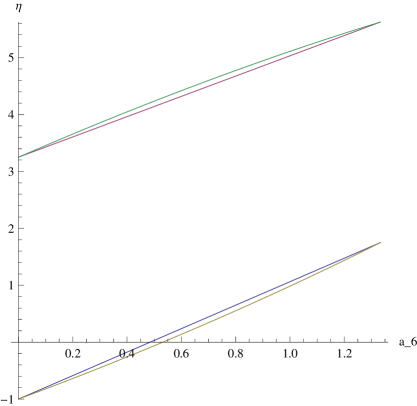
Figure 2: Trajectories $\eta(a_{6}),$ see Eq. (21), for the toy model for a Slater determinant, as described in the text.

While usually many wave functions can give the same density, this toy model allows the wave function to be identified. It is that Slater determinant $\Phi_{gs}$ made of $\varphi_{0}$ and $\varphi_{1}.$ This $\Phi_{gs}$ is, obviously, the first two-fermion eigenstate of our $K,$ a sum of two harmonic oscillators, with eigenvalue, $2=1/2+3/2.$ The same $\Phi_{gs}$ is also an eigenstate of $V,$ Eq. (7), since in the following Jacobi coordinates, $R=(r_{1}+r_{2})/2,$ $r_{21}=r_{2}-r_{1},$ the wave function of $\Phi_{gs}$ reads, $\propto\exp(-R^{2})\ r_{21}\,\exp(-r_{21}^{2}/4),$ while the representation of $V$ is, $\langle Rr_{21}|V|R^{\prime}r^{\prime}_{21}\rangle\propto\delta(R-R^{\prime})\ r_{21}\,r^{\prime}_{21}\,\exp[-(r_{21}^{2}+r_{21}^{\prime 2})/4],$ showing an obvious projector on that relative motion expressed by $\Phi_{gs}.$ The corresponding eigenvalue is, $-V_{0},$ hence our result, $\eta=-1,$ when $V_{0}=3.$ We took great care to verify that the same results are obtained if, instead of $a_{6},$ we use other choices for “density constraint”, such as the parameter $a_{0},$ or a moment such as the second one, $a_{0}/2+3a_{2}/4+15a_{4}/8+105a_{6}/16,$ or the local value $\rho(\theta)$ at some testing point $r=\theta.$ Such rearrangements of information with respect to the wave function parameters may be of some interest for questions of physics or numerical convenience, but do not change the nature of the algebra nor the the final results. It can be noted here that what is important for the method is that the energy and the constraints be polynomials of the parameters. The fact that, in the toy model, the density is described by a polynomial of $r$ is not essential. It only makes the algebra slightly simpler. With wave functions more complicated than harmonic oscillator ones, any choice of moments, or local values of $\rho,$ still makes eligible constraints.

An issue which will arise in all future models using this polynomial method is that the final minimization of $\eta$ must be performed within a convex domain of densities: what conditions must the coefficients $a_{i},$ or those other selected parameters (moments, local values, etc), satisfy to maintain $\rho$ positive? This question was recently GiPe solved by means of the Sturm criterion, for a general class of positive functions having positive Fourier transforms. The criterion gives the number of real roots of a polynomial, and can be used to ensure that a polynomial has no real roots. As seen in the toy model, the detailed structure of the calculation can be a guide to define the physically acceptable domain of parameters, see the bounds found for $a_{6}$ and $a_{0}.$ For more subtle questions about the topology of acceptable functional spaces of densities and trial functions, we refer to UllKohtopo , but will conjecture, without proof, that here with traditional functions (harmonic, Coulomb) and their configuration mixings, the positivity of $\rho$ should be sufficient.

There is also the question of spurious solutions. The elimination of that spurious solution found in the Slater toy model turned out to be trivial. For more complicated systems, spurious solutions Har ; PBLB might certainly pop up, but an analysis for their detection remains easy. In particular, for other toy models that we tested, spurious solutions were found to induce values of physical parameters out of their allowed range, and/or even complex values while only real ones are acceptable. We can insist that the final, polynomial equation for the energy, $\mathcal{S}(\eta)=0,$ can only create a finite number of candidate solution branches to be investigated.

This concludes our toy model as a demonstration of a handling of determinants in this algebraic approach. But we can still take advantage of it for a study of the “kinetic Kohn-Sham functional”. First notice that the “harmonic energy”, $\langle\Phi|K|\Phi\rangle,$ and the kinetic energy of $\Phi$ differ by only an explicit functional of the density, namely half of its second moment, $\int dr\,r^{2}\,\rho(r).$ The search for a functional for $\langle\Phi|K|\Phi\rangle,$ therefore, is a problem equivalent to that for the kinetic energy. Set now $V_{0}=0$ in Eqs. (19). The same program of elimination that was used for a full energy functional now returns a simpler, and very transparent, form of Eq. (22), $(\eta-6)(\eta-4)^{2}(\eta-2)=0.$ The corresponding version of Eq. (21), $(2\eta-4-3a_{6})^{2}\,(2\eta-8-3a_{6})^{2}=0,$ gives $\eta=2$ and $\eta=4$ if $a_{6}=0.$ This means determinants made of $\{\varphi_{0},\varphi_{1}\}$ and $\{\varphi_{2},\varphi_{1}\},$ respectively. For $a_{6}=4/3,$ at the other edge of the domain, the harmonic energies are $\eta=4$ and $\eta=6,$ with determinants $\{\varphi_{0},\varphi_{3}\}$ and $\{\varphi_{2},\varphi_{3}\},$ respectively.

After this proof that the method is basically the same for determinants as for configuration mixings, we can stress that configuration mixings have the technical advantage that the energy is quadratic only and permits the short cut described at the stage of Eqs (5,6).

A constructive derivation of KSPs is available. For instance, truncate some single particle basis and let $\mathcal{P}$ be the projector upon the resulting, finite dimensional subspace for a system of $N$ fermions, with their Hamiltonian $H$, or rather now, $\mathcal{P}H\mathcal{P}$. Given the kinetic energy operator $T,$ choose a local potential $w_{0}(r),$ hence a one-body operator $W_{0}=\sum_{i=1}^{N}w_{0}(r_{i})$, hence a one-body Hamiltonian $H_{0}=T+W_{0}$, so that the ground state of $\mathcal{P}H_{0}\mathcal{P}$, a Slater determinant $\Phi_{0}$, be non degenerate and providing an approximate density $\rho_{0}$ for the system. For any density $\rho$ in the subspace, the integral, $\int\Delta\rho$, of the difference, $\Delta\rho=\rho-\rho_{0}$, vanishes as already stated. (Here and in the following, the integral sign, $\int$, means $\int r^{d-2}\,dr$ depending on the $d$-dimensional problem under consideration.) Expand, as already discussed, $\Delta\rho$ in a basis of orthonormal functions $S_{\beta}(r)$, “constrained by vanishing averages” Gi05 ; Nor , $\Delta\rho(r)=\sum_{\beta=1}^{\infty}b_{\beta}\,S_{\beta}(r).$ Truncate the expansion at some suitable order $\mathcal{N}^{\prime}.$ Again, given a determinant $\Phi$ with the parameters $c_{n\ell m}^{\alpha}$ of its orbitals, or given a correlated state, $\Psi=\sum_{q}C_{q}\,\Phi_{q}$, the constraints, $\Phi\Rightarrow b_{\beta}$ or $\Psi\Rightarrow b_{\beta}$, are polynomials of the parameters. Given $H_{0}$, the polynomial method returns a polynomial $\mathcal{K}(\kappa,b_{1},\dots,b_{\mathcal{N}^{\prime}})$ for a reference functional, such that the lowest root of the equation, $\mathcal{K}=0$, represents the constrained minimum, $\kappa^{\prime}=\mathrm{Min}_{\Phi\Rightarrow b_{1},\dots,b_{\mathcal{N}^{\prime}}}\langle\Phi|H_{0}|\Phi\rangle$, for the determinants in the subspace. In the same way, given the full $H$, the method gives a polynomial $\mathcal{E}(\eta,b_{1},\dots,b_{\mathcal{N}^{\prime}}),$ the lowest $\eta$ root of which is the constrained minimum, $\eta^{\prime}=\mathrm{Min}_{\Psi\Rightarrow b_{1},\dots,b_{\mathcal{N}^{\prime}}}\langle\Psi|H|\Psi\rangle$, for correlated states in the subspace. Then it is trivial to derive from $\mathcal{K}$ and $\mathcal{E}$ a polynomial, $\Omega(\omega;b_{1},\dots,b_{\mathcal{N}^{\prime}})$, for the difference, $\omega=\eta-\kappa$. The diagonalization of $\mathcal{P}H\mathcal{P}$ then reads,

$$\frac{\partial\kappa}{\partial b_{\beta}}+\frac{\partial\omega}{\partial b_{\beta}}=0,\ \ \beta=1,\dots,\mathcal{N}^{\prime}.$$ (25)

With the ratio, $v_{\beta}=-(\partial\Omega/\partial b_{\beta})/(\partial\Omega/\partial\omega)$, representing $\partial\omega/\partial b_{\beta}$, define the one-body, local potential, $v_{\Delta}(r)=\sum_{\beta=1}^{\mathcal{N}^{\prime}}v_{\beta}\,S_{\beta}(r)$. Let $\Phi$ be the ground state of $\mathcal{P}\left[H_{0}+\sum_{i=1}^{N}v_{\Delta}(r_{i})\right]\mathcal{P}.$ Notice that $\langle\Phi|\mathcal{P}S_{\beta}\mathcal{P}|\Phi\rangle=\langle\Phi|S_{\beta}|\Phi\rangle.$ Then the energy $E$ of $\Phi$ has derivatives,

$$\partial E/\partial v_{\beta}=\int(\Delta\rho+\rho_{0})\,S_{\beta}=b_{\beta}+b_{\beta 0},$$ (26)

because of the orthonormality of the $S_{\beta}$’s. The numbers, $b_{\beta 0}=\int\rho_{0}\,S_{\beta}$, are easily pretabulated. The quantities, $v_{\beta}$ and $(b_{\beta}+b_{\beta 0})$, are Legendre conjugates, and, moreover, $\partial/\partial(b_{\beta}+b_{\beta 0})=\partial/\partial b_{\beta}$. The conditions, Eqs. (25), read as the diagonalization for a determinant $\Phi$ with the same density $\rho$ as that of the eigenstate $\Psi$ of $\mathcal{P}H\mathcal{P}$. The potential, $\mathcal{P}(w_{0}+v_{\Delta})\mathcal{P}$, is a KSP valid for the subspace, up to the convergence of the truncation with $\mathcal{N}^{\prime}$ terms.

This polynomial method most often uses a very non local parametrization of $\rho,$ that deviates from the quasi-local tradition of the field. In every case, our unconventional parametrization of $\rho$ creates a new zoology of DFs. Nothing of this zoology is known to us, but its interest is obvious, since manipulations of polynomials and properties of their roots, including bounds, are basic subjects. Moreover, extrapolations of polynomials, and criticism of such extrapolations, are easy. The number of available, exactly solvable models is huge. It is limited only by computational power. For nuclei or atoms, the models will be “radial” GirRDF , somewhat simple. For nuclear physics, our ultimate goal will be to see whether particle number can be used as a constraint, to generate a mass formula. For electrons in molecules or extended systems (metals, thin layers, etc.), however, a necessary algebra of functions of 2 or 3 variables will burden the models. Anyhow, one can always test whether our polynomials from “smaller” models may remain good approximations for “larger” ones, if, for instance, scaling properties can be established. Asymptotic properties of a sequence of “DF polynomials” might guide towards derivations of more traditional DFs. In particular, the polynomial models allow comparisons between the KS and the true kinetic energies of correlated systems. They also provide explicit terms for those correlation energies due to interactions.

In conclusion, this algebraic method simplifies density functional theory into energy minimization under finite numbers of constraints, under very elementary manipulations of polynomials. It retains all essential information about the density and all components of the energy. In a forthcoming paper, we shall investigate a more realistic problem than the toy models used for this Letter.

SK acknowledges support from the National Research Foundation of South Africa and thanks CEA/Saclay for hospitality during part of this work. BG thanks Rhodes University and the University of Johannesburg for their hospitality during part of this work.

References

• (1) P. Hohenberg and W. Kohn, Phys. Rev. 136, B864 (1964).
• (2) W. Kohn and L. J. Sham, Phys. Rev. 140, A1133 (1965).
• (3) J. Harris and R.O. Jones, J. Phys. F 4 1170 (1974).
• (4) F. Colonna and A. Savin, J. Chem. Phys. 110 2828 (1999).
• (5) A.M. Teale, S. Coriani and T. Helgaker, J. Chem. Phys. 130 10411 (2009).
• (6) J.T. Chayes, L. Chayes and M.B. Ruskai, J. Stat. Phys. 38 497 (1985).
• (7) J.E. Hariman, Phys. Rev. A 27 632 (1983).
• (8) R. Pino, O. Bokanowski, E.V. Ludena and R.L. Boada, Theor. Chem. Acc. 123 189 (2009).
• (9) J. Katriel, C.J. Appellof and E.R. Davidson, Int. J. Quant. Chem. 19 293 (1981).
• (10) R.M. Dreizler and E.K.U. Gross, Density Functional Theory, Springer, Berlin/Heidelberg (1990); see also the references in their review.
• (11) R.G. Parr and W. Yang, Annu. Rev. Phys. Chem. 46 701 (1995).
• (12) J. E. Drut, R. J. Furnstahl, and L. Platter, Prog. Part. Nucl. Phys. 64, 120 . (2010).
• (13) B.G. Giraud, Phys. Rev. C 78 014307 (2008).
• (14) M. Levy, Proc. Natl. Acad. Sci. USA76 6062 (1979); E. H. Lieb, Int. J. Quantum Chem. 24 243 (1983).
• (15) B.G. Giraud, A. Weiguny and L. Wilets, Nucl. Phys. A 761 22 (2005); B.G. Giraud, J. Phys. A 38 7299 (2005).
• (16) J.M. Normand, J. Phys. A 40 2341 and 2371 (2007).
• (17) J.P. Perdew and M. Levy, Phys. Rev. 31 6264 (1985).
• (18) B.G. Giraud and R. Peschanski, Acta Phys. Pol. B 37 331 (2006).
• (19) C. A. Ullrich and W. Kohn, Phys. Rev. Lett. 89 156401 (2003).