Nonequilibrium thermal entanglement in three-qubit $XX$ model

Abstract

Making use of the master equation and effective Hamiltonian approach, we investigate the steady state entanglement in a three-qubit $XX$ model. Both symmetric and nonsymmetric qubit-qubit couplings are considered. The system (the three qubits) is coupled to two bosonic baths at different temperatures. We calculate the steady state by the effective Hamiltonian approach and discuss the dependence of the steady state entanglement on the temperatures and couplings. The results show that for symmetric qubit-qubit couplings, the entanglements between the nearest neighbor are equal, independent of the temperatures of the two baths. The maximum of the entanglement arrives at $T_{L}=T_{R}$. For nonsymmetric qubit-qubit couplings, however, the situation is totally different. The baths at different temperatures would benefit the entanglement and the entanglements between the nearest neighbors are no longer equal. By examining the probability distribution of each eigenstate in the steady state, we present an explanation for these observations. These results suggest that the steady entanglement can be controlled by the temperature of the two baths.

When we talk about a real physical system, we should take the effects of its environment into account because all quantum systems interact unavoidably with their surroundings. A quantum system that can not isolate from its environment is usually referred to open quantum system BPbookprojection . The dynamics of open quantum systems can be described by quantum master equations in the Schrödinger picture, or Langevin equation in the Heisenberg picture quantumoptics . The coupling of environment to a system definitely changes the properties of the system, such as the geometric phase Berry and entanglement Entanglement1935 .

Entanglement is a quantum resource that has no classical counterpart. It was first recognized in 1935, and has been widely studied in recent years due to its potential applications in quantum information processing nielsen . The environment can either induce entanglement induceE or decrease entanglement (in this case environment often lead to a death of entanglement, which is usually called entanglement sudden death ESD ). When a quantum system is in contact with a heat reservoir at a fixed temperature, the system will relax into a thermal equilibrium state $\rho(T){=}e^{-\beta H}/\text{Tr}(e^{-\beta H})$ eventually. The entanglement of this state is called thermal entanglement, which has been extensively studied in the past decade thermalE .

In this paper, we shall study a different type of thermal entanglement. It depends on temperature but its state is not statistically equilibrium. This situation arises when a quantum system interacts with two bosonic baths at different temperatures. The state of the quantum system eventually arrived is not a statistically equilibrium but a steady state steadystateNon . In Ref.Yan0809PRB , the heat transport were studied for such a system. In Ref.NTE2007 , the entanglement of a two qubit $XX$ chain were studied for both identical and different qubits. In this paper, we will study the entanglement of a three qubit $XX$ chain coupled to two baths at different temperatures. Two cases, i.e., symmetric and nonsymmetric qubit-qubit couplings, are considered.

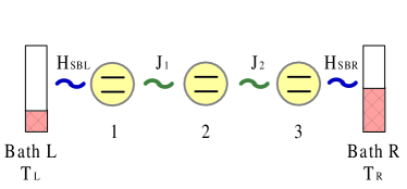
Figure 1: A schematic representation of our model. The two-level systems are connected to two bosonic baths held at different temperatures, $T_{L}$ and $T_{R}$, respectively.

Consider a spin chain consisting of three spins with $XX$ interaction. The Hamiltonian for this system has the form,

$$H{=}\sum_{n=1}^{3}\frac{\varepsilon}{2}\sigma^{z}_{n}{+}J_{1}(\sigma^{+}_{1}\sigma^{-}_{2}{+}\sigma^{-}_{1}\sigma^{+}_{2}){+}J_{2}(\sigma^{+}_{2}\sigma^{-}_{3}{+}\sigma^{-}_{2}\sigma^{+}_{3}),$$ (1)

where $\sigma^{z}_{n}$ and $\sigma^{\pm}_{n}$ are Pauli operators for the $n$th spin, and $J_{1}$ and $J_{2}$ denote coupling constants. Spin 1 and 3 interact with two sperate bosonic baths at different temperatures $T_{L}$ and $T_{R}$, respectively (see Fig.1). The Hamiltonian for each bath $j{=}L,R$ is given by $H_{Bj}{=}\sum_{n}\omega_{n,j}b^{{\dagger}}_{n,j}b_{n,j}$ and the interaction between the spin and its bath is described by $H_{SBj}{=}\sigma^{+}_{j}\sum_{n}g_{n}^{(j)}b_{n,j}{+}\sigma^{-}_{j}\sum_{n}g_{n}^{(j)}b_{n,j}^{{\dagger}}=\sum_{\mu}X_{j,\mu}^{+}\Gamma_{j,\mu}{+}X_{j,\mu}^{-}\Gamma_{j,\mu}^{{\dagger}}$ ($j=1,3$ for spin), here the operator $X_{j,\mu}$ is an eigenoperator of the system Hamiltonian satisfying $[H,X_{j,\mu}^{\pm}]{=}\pm\omega_{j,\mu}X_{j,\mu}^{\pm}$, and $\Gamma_{j,\mu}$ acts on the bath degrees of freedom. We assume the both baths are in the uncorrelated thermal equilibrium states. Then the density operator of the bath is $\rho_{Bj}{=}e^{-\beta_{j}H_{Bj}}/\text{Tr}(e^{-\beta_{j}H_{Bj}})$. In this paper we set $k_{B}{=}\hbar{=}1$ for simplicity. Under this assumption, the dimension of the transition frequency $\varepsilon$, coupling constants $J_{1},J_{2}$ and the temperatures $T_{L},T_{R}$ are same. In our following discussion, the value of these parameters only stand for the ration relation between them. The dynamics of the system affected by the two baths can be described by the quantum master equation quantumoptics , which is obtained by tracing out the bath variables within the Born-Markovian approximation. This equation can usually be arranged in Lindblad form

$$\frac{\partial}{\partial t}\rho=-i[H,\rho]+\mathcal{L}_{L}\rho+\mathcal{L}_{R}\rho,$$ (2)

where $\mathcal{L}_{L}\rho$ ($\mathcal{L}_{R}\rho$) is the dissipative term due to the coupling of the system to the left (right) bath. In order to find an exact form of the dissipative term, we go to the bases composed by the eigenstates $|s_{i}\rangle$ of the system Hamiltonian with the corresponding eigenvalues $\lambda_{i}$

$$|s_{1}\rangle{=}|111\rangle,\lambda_{1}{=}\frac{3}{2}\varepsilon,$$

$$|s_{2}\rangle{=}|000\rangle,\lambda_{2}{=}-\frac{3}{2}\varepsilon,$$

$$|s_{3}\rangle{=}\frac{\sqrt{2}}{2}(\sin\theta|110\rangle{-}|101\rangle{+}\cos\theta|011\rangle),\lambda_{3}{=}\frac{1}{2}\varepsilon{-}J,$$

$$|s_{4}\rangle{=}\cos\theta|110\rangle{-}\sin\theta|011\rangle,\lambda_{4}{=}\frac{1}{2}\varepsilon,$$

$$|s_{5}\rangle{=}\frac{\sqrt{2}}{2}(\sin\theta|110\rangle{+}|101\rangle{+}\cos\theta|011\rangle),\lambda_{5}{=}\frac{1}{2}\varepsilon{+}J,$$

$$|s_{6}\rangle{=}\frac{\sqrt{2}}{2}(\cos\theta|100\rangle{-}|010\rangle{+}\sin\theta|001\rangle),\lambda_{6}{=}{-}\frac{1}{2}\varepsilon{-}J,$$

$$|s_{7}\rangle{=}\sin\theta|100\rangle{-}\cos\theta|001\rangle,\lambda_{7}{=}{-}\frac{1}{2}\varepsilon,$$ (3)

$$|s_{8}\rangle{=}\frac{\sqrt{2}}{2}(\cos\theta|100\rangle{+}|010\rangle{+}\sin\theta|001\rangle),\lambda_{8}{=}{-}\frac{1}{2}\varepsilon{+}J,$$

where $J{=}\sqrt{J_{1}^{2}+J_{2}^{2}}$, and $\tan\theta{=}\frac{J_{2}}{J_{1}}$. In this representation, the dissipative term $\mathcal{L}_{j}\rho$ ($j{=}L,R$) can be written as

$$\mathcal{L}_{j}\rho=\sum_{\mu=1}^{3}J^{(j)}(-\omega_{\mu})\left(2X_{j,\mu}\rho X_{j,\mu}^{{\dagger}}-\{\rho,X_{j,\mu}^{{\dagger}}X_{j,\mu}\}\right)$$

$$+J^{(j)}(\omega_{\mu})\left(2X_{j,\mu}^{{\dagger}}\rho X_{j,\mu}-\{\rho,X_{j,\mu}X_{j,\mu}^{{\dagger}}\}\right),$$ (4)

with eigenfrequencies,

$$\omega_{1}=\varepsilon+J,~{}~{}~{}~{}\omega_{2}=\varepsilon,~{}~{}~{}~{}\omega_{3}=\varepsilon-J,$$ (5)

and corresponding eigenoperators

$$X_{L,1}=\frac{\sqrt{2}}{2}\cos\theta|s_{3}\rangle\langle s_{1}|-\frac{1}{2}|s_{6}\rangle\langle s_{4}|$$

$$~{}~{}~{}~{}~{}~{}~{}~{}~{}~{}~{}-\frac{\sqrt{2}}{2}\cos\theta|s_{7}\rangle\langle s_{5}|+\frac{\sqrt{2}}{2}\cos\theta|s_{2}\rangle\langle s_{8}|,$$

$$X_{L,2}=-\frac{\sqrt{2}}{2}|s_{4}\rangle\langle s_{1}|-\sin\theta|s_{6}\rangle\langle s_{3}|$$

$$~{}~{}~{}~{}~{}~{}~{}~{}~{}~{}~{}+\sin\theta|s_{8}\rangle\langle s_{5}|+\sin\theta|s_{2}\rangle\langle s_{7}|,$$

$$X_{L,3}=\frac{\sqrt{2}}{2}\cos\theta|s_{5}\rangle\langle s_{1}|+\frac{\sqrt{2}}{2}\cos\theta|s_{7}\rangle\langle s_{3}|$$

$$~{}~{}~{}~{}~{}~{}~{}~{}~{}~{}~{}+\frac{1}{2}|s_{8}\rangle\langle s_{4}|+\frac{\sqrt{2}}{2}\cos\theta|s_{2}\rangle\langle s_{6}|,$$

$$X_{R,1}=\frac{\sqrt{2}}{2}\sin\theta|s_{3}\rangle\langle s_{1}|+\frac{1}{2}|s_{6}\rangle\langle s_{4}|$$

$$~{}~{}~{}~{}~{}~{}~{}~{}~{}~{}~{}+\frac{\sqrt{2}}{2}\sin\theta|s_{7}\rangle\langle s_{5}|+\frac{\sqrt{2}}{2}\sin\theta|s_{2}\rangle\langle s_{8}|,$$

$$X_{R,2}=\frac{\sqrt{2}}{2}|s_{4}\rangle\langle s_{1}|-\cos\theta|s_{6}\rangle\langle s_{3}|$$

$$~{}~{}~{}~{}~{}~{}~{}~{}~{}~{}~{}+\cos\theta|s_{8}\rangle\langle s_{5}|-\cos\theta|s_{2}\rangle\langle s_{7}|,$$

$$X_{R,3}=\frac{\sqrt{2}}{2}\sin\theta|s_{5}\rangle\langle s_{1}|-\frac{\sqrt{2}}{2}\sin\theta|s_{7}\rangle\langle s_{3}|$$

$$~{}~{}~{}~{}~{}~{}~{}~{}~{}~{}~{}-\frac{1}{2}|s_{8}\rangle\langle s_{4}|+\frac{\sqrt{2}}{2}\sin\theta|s_{2}\rangle\langle s_{6}|.$$ (6)

The spectral density in Eq.(4) is defined by

$$J^{(j)}(\omega_{\mu})=\int_{0}^{\infty}d\tau e^{i\omega_{j,\mu}}\left\langle e^{-iH_{Bj}\tau}\Gamma^{{\dagger}}_{j,\mu}e^{iH_{Bj}\tau}\Gamma_{j,\mu}\right\rangle.$$ (7)

In this paper, the bath is assumed as an infinite set of harmonic oscillators, so the spectral density has the form $J^{(j)}(\omega_{\mu}){=}\gamma_{j}(\omega_{\mu})n_{j}(\omega_{\mu})$, where $n_{j}(\omega_{\mu}){=}(e^{\beta_{j}\omega_{\mu}}{-}1)^{-1}$ and $J^{(j)}(-\omega_{\mu}){=}e^{\beta_{j}\omega_{\mu}}J^{(j)}(\omega_{\mu})$. On the same footing as the Born-Markovian approximation, we take here a Weisskopf-Winger form for the coupling constant as $\gamma_{j}(\omega_{\mu}){=}\gamma_{j}$, i.e., the coupling constant is spectrum independent.

The master equation can be solved by the fourth-order Runge-Kutta method and the steady state can be reached when we set the evolution time long enough Yan0809PRB . Different from this method, we solve the steady state of Eq.(2) here with the help of effective Hamiltonian approach EHAall . The main idea of this method can be described as follows. By introducing an ancilla, we map the density matrix and the master equation to a state vector and a Schrödinger-like equation. The solution of the master equation can be obtained by mapping the solution of the Schrödinger-like equation back to the density matrix. Rewrite the master equation in the Lindblad form Lindblad as $\frac{\partial}{\partial t}\rho{=}-i[H,\rho]{-}\frac{1}{2}\sum_{k}\left(L_{k}^{{\dagger}}L_{k}\rho{+}\rho L_{k}^{{\dagger}}L_{k}{-}2L_{k}\rho L_{k}^{{\dagger}}\right)$. Then the effective Hamiltonian is defined by $\mathcal{H}_{T}=H{-}H^{A}{-}\frac{i}{2}\sum_{k}L_{k}^{{\dagger}}L_{k}{-}\frac{i}{2}\sum_{k}L_{k}^{A{\dagger}}L_{k}^{A}{+}i\sum_{k}L_{k}^{A}L_{k}$, where $A$ denotes the operator for the ancilla, which is defined by $\langle e_{m}|O^{A}|e_{n}\rangle{=}\langle E_{n}|O^{{\dagger}}|E_{m}\rangle$. Here $\{|E_{n}\rangle\}$ and $\{|e_{n}\rangle\}$ are time independent bases for the original system and the ancilla. The initial state independent steady state corresponding to the eigenstate of $\mathcal{H}_{T}$ with eigenvalue zero. Then we can study the steady state properties for such a system.

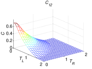
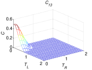
Figure 2: Steady state entanglement $C_{12}$ and $C_{13}$ as functions of the bath temperatures $T_{L}$ and $T_{R}$. Here $\varepsilon{=}1$ and $J_{1}{=}J_{2}=1$.

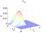
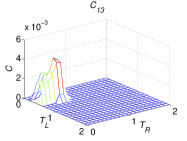
Figure 3: Steady state entanglement $C_{12}$ and $C_{13}$ as functions of the bath temperatures $T_{L}$ and $T_{R}$. Here $\varepsilon{=}3$ and $J_{1}{=}J_{2}{=}1$.

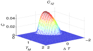
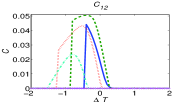
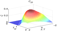
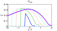
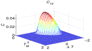
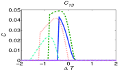
Figure 4: (Color online) Left column, the steady state entanglement as functions of the mean bath temperature $T_{M}{=}(T_{L}{+}T_{R})/2$ and the temperature difference $\Delta T{=}T_{L}{-}T_{R}$ in non-symmetrical case. Right column shows the corresponding concurrences change with $\Delta T$ in the case of $T_{M}{=}0.2$ (blue-solid), $T_{M}{=}0.4$ (green-dashed), $T_{M}{=}0.6$ (red-dotted), $T_{M}{=}0.8$ (cyan-dash-dot), and $T_{M}{=}1$ (pink-circle). Here $\varepsilon{=}3$, $J_{1}{=}0.5$ and $J_{2}{=}2.5$.

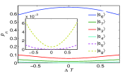
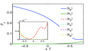
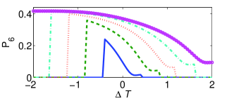
Figure 5: (Color online) The probability distribution for eigenstates $|s_{i}\rangle,i{=}3,4,\cdots,8$ in the steady state as a function of the temperature difference $\Delta T$. In top-left figure we set $\varepsilon{=}1$ and $J_{1}{=}J_{2}{=}1$, while in top-right figure we choose $\varepsilon{=}3$, $J_{1}{=}0.5$ and $J_{2}{=}2.5$. In both two figures, the mean bath temperature $T_{M}$ is fixed with $T_{M}{=}0.4$. In bottom figure, we plot the probability distribution for $|s_{6}\rangle$ with different mean bath temperature. The mean bath temperatures correspond to the right column of Fig.4.

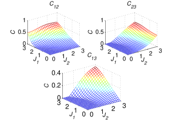
Figure 6: Steady state entanglement as functions of the coupling strength $J_{1}$ and $J_{2}$ in the case $\varepsilon{=}3$, $T_{M}{=}0.5$, $\Delta T{=}-0.4$.

Choosing the concurrence concurrence as the measure of entanglement, we first study the steady state concurrence in the case of symmetric qubit-qubit couplings ($J_{1}{=}J_{2}$). In Figs.2 and 3, we plot the steady state concurrence $C_{12}$ (entanglement between spins 1 and 2), and $C_{13}$ (entanglement between spins 1 and 3) at different temperatures $T_{L}$ and $T_{R}$. In Fig.2, we set $\varepsilon{=}1$ and in Fig.3, $\varepsilon{=}3$. The coupling strength are chosen to be $J_{1}{=}J_{2}{=}1$. Some features can be observed from the figures. First, although the value of $C_{12}$ and $C_{13}$ are quite different, the tendencies of them affected by $T_{L}$ and $T_{R}$ are similar. The other interesting feature is that, in both Fig.2 and Fig.3, $C_{12}$ and $C_{13}$ are symmetric about $T_{L}{=}T_{R}$, and the peak(maximum) appears when $T_{L}{=}T_{R}$. This means that, $C_{12}{=}C_{23}$ holds in this case. In other words, the entanglements between the nearest neighbors are equal although the two temperatures are different. Moreover the larger the temperature difference, the smaller the entanglement.

In nonsymmetric case ($J_{1}{\neq}J_{2}$), the results are quite different. We first plot the concurrences between any two spins as functions of the mean bath temperature $T_{M}{=}\frac{1}{2}(T_{L}{+}T_{R})$ and the temperature difference $\Delta T{=}T_{L}{-}T_{R}$ in Fig.4. The parameters in the figure are chosen $\varepsilon{=}3$, $J_{1}{=}0.5$ and $J_{2}{=}2.5$. It can be easily seen from the figure that the peak does not appear at $\Delta T{=}0$ (For more clearly, see the right column of Fig.4), i.e., for a fixed value of mean bath temperature, the peak appears at the points where the temperature difference is not zero, suggesting that temperature difference benefits the entanglement in nonsymmetric case. If one wants to get a larger entanglement when the qubit-qubit couplings are not equal, a specific temperature difference is necessary. The other interesting phenomenon in this case is that when the difference between the coupling constant $J_{1}$ and $J_{2}$ is large enough (for example, in our figure $J_{1}{=}0.5$, $J_{2}{=}2.5$), the difference between $C_{12}$ and $C_{13}$ becomes negligible. In other words, $C_{13}$, the concurrence between the next-to-nearest neighbor qubits, tends to the concurrence between the nearest neighbors with weak coupling (in our condition, $C_{12}$), and they all are smaller than that in the case with stronger couplings (in our condition, $C_{23}$).

To understand these features, we calculate the probability distribution for the eigenstates of the Hamiltonian $H$ in the steady state, this distribution is a function of temperature difference $\Delta T$ as shown in Fig.5. Although the entanglement does not satisfy the role of superpositionentsuperposition , the probability distribution are helpful to understand the features we found in the entanglement. In the top-left figure of Fig.5, we plot this distribution for the symmetric case, i.e., $J_{1}{=}J_{2}=1$. The other parameters are $\varepsilon{=}1$, $T_{M}{=}0.4$. From the figure, we find that the probability distributions for all the eigenstates are symmetrical about $\Delta T{=}0$, and $|s_{6}\rangle,|s_{3}\rangle$ dominate the distribution. The distribution for $|s_{1}\rangle$ and $|s_{2}\rangle$ are not shown in this figure, because these two states are separable. On the other hand, for symmetric couplings we have $\tan\theta{=}1$, then the eigenstates can be divided into two parts, i.e., symmetric eigenstates $|s_{3}\rangle,|s_{5}\rangle,|s_{6}\rangle,|s_{8}\rangle$, and antisymmetric eigenstates $|s_{4}\rangle$ and $|s_{7}\rangle$. By symmetric we mean the state remains unchanged when one exchanges the particles 1 and 3, hence for symmetric state the entanglement between particles (1,2) and (2,3) equals. For the antisymmetric states, it is easy to check that these is no entanglement between particle (1,2) or (2,3). These observations for the eigenstates together with their distribution in the steady, we can conclude that the entanglement between the nearest neighbors are equal although the two temperatures for the two baths are different, this analysis confirms the numerical simulation presented in the figure.

The top-right figure in Fig.5 shows the probability distribution for the nonsymmetric case. We have set $\varepsilon{=}3$, $J_{1}{=}0.5$ and $J_{2}{=}2.5$. From this figure, we find that entanglement in the steady states is mainly determined by the state $|s_{6}\rangle$. We plot the probability distribution of $|s_{6}\rangle$ with different mean bath temperature in the bottom of Fig.5. Now we analyze the entanglement properties for this state. By tracing out one particle from the state $|s_{6}\rangle$, we can easily obtain the concurrence for the remaining two spins as $C_{12}{=}\cos\theta$, $C_{13}{=}\cos\theta\sin\theta$ and $C_{23}{=}\sin\theta$. In nonsymmetric case, for example, $J_{1}{=}0.5,J_{2}{=}2.5$, we have $\tan\theta{=}5$, which results in $\sin\theta{\simeq}1$. This is the reason why $C_{12}{\simeq}C_{13}$ in Fig.4 and they are much smaller than $C_{23}$. Moreover, observing the distribution probability for $|s_{6}\rangle$ (blue line in the middle figure of Fig.5 and the bottom figure), we can find that the peak of entanglement does not appear at $\Delta T{=}0$ in nonsymmetric case, namely the temperature difference favors the steady state entanglement.

Finally we study the effect of two coupling constant on the concurrence for fixed bath temperature. In Fig.6, we show the concurrences as functions of $J_{1}$ and $J_{2}$ with $\varepsilon{=}3$, $T_{M}{=}0.5$ and $\Delta T{=}-0.4$. Both $J_{1}$ and $J_{2}$ enhance the entanglement. This enhancement is more strikingly in the case of $J_{1}$ for $C_{12}$ while $J_{2}$ for $C_{23}$. Due to the temperature difference, $C_{13}$ is not symmetric about $J_{1}{=}J_{2}$.

In summary, we have studied the steady state entanglement in a three-qubit $XX$ model. The qubits are coupled to two independent bosonic baths at different temperatures. With the help of the effective Hamiltonian approach, we have calculated the steady state entanglement and discussed its dependence on temperatures and couplings. Two types of the coupling, i.e., symmetric and nonsymmetric one are considered. When the coupling is symmetric, we find that the entanglement between the nearest neighbors, i.e., $C_{12}$ and $C_{23}$, are equal though the temperatures of the two baths are different. The maximum of entanglement is found when the temperatures of the two baths are equal. For the nonsymmetric case, however, the maximal entanglement arrives when the two baths at different temperatures. By analyzing the distribution for each eigenstate, we qualitatively explain these interesting phenomena. The dependence of the entanglement on the coupling constants are also presented and discussed.

We thank Dr H. T. Cui for discussion. This work is supported by NSF of China under grant Nos. 10775023 and 10935010.

References

(1) H. P. Breuer et al.The Theory of Open Quantum Systems (Oxford University Press,
Oxford 2002).
(2) M. O. Scully et al.Quantum
Optics (Cambridge University Press, Cambridge 1997); D. F. Walls
et al.Quantum Optics (Springer, Berlin,1994).
(3) M. V. Berry, Proc. R. Soc. London A 392, 45
(1984); B. Simon, Phys. Rev. Lett. 51, 2167 (1983); Y.
Aharonov et al. Phys. Rev. Lett. 58, 1593 (1987); J.
Samuel et al. Phys. Rev. Lett. 60, 2339 (1988); E.
Sjöqvist et al. Phys. Rev. Lett. 85, 2845 (2000);
D. M. Tong et al. Phys. Rev. Lett. 93, 080405 (2004);
I. Kamleitner et al. Phys. Rev. A 70, 044103
(2004); A. Bassi
et al. Phys. Rev. A 73, 062104
(2006); F. C. Lombardo et al.
Phys. Rev. A 74, 042311
(2006); A. Carollo et al.
Phys. Rev. Lett. 96, 150403
(2006); X. X. Yi et al.
Phys. Rev. A 73, 052103
(2006); A. T. Rezakhani et al.,
Phys. Rev. A 73, 052117
(2006); X. L. Huang et al.,
EPL 82, 50001 (2008).
(4) A. Einstein, et al. Phys.
Rev. 47, 777 (1935); E. Schrödinger, Proc. Cambridge
Philos. Soc. 31, 555 (1935).
(5) See, e.g. M. A. Nielsen et al.Quantum Computation and Quantum
Information (Cambridge University Press, Cambridge,2000).
(6) M. B. Plenio et al.
Phys. Rev. Lett. 88, 197901
(2002); D. Braun Phys. Rev. Lett. 89, 277901
(2002); X. X. Yi,
et al. Phys. Rev. A 68, 052304
(2003).
(7) Ting Yu et al. Phys. Rev. Lett. 93, 140404
(2004).
(8) M. C. Arnesen et al.
Phys. Rev. Lett. 87, 017901
(2001); X. G. Wang, Phys. Rev. A 64, 012313
(2001); X. G.
Wang et al. J. Phys. A 34, 11307 (2001); X. G. Wang,
Phys. Lett. A 281, 101 (2001); X. G. Wang, Phys. Rev. A 66, 034302
(2002); X. G.
Wang, Phys. Rev. A 66, 044305
(2002); G. L. Kamta et al.
Phys. Rev. Lett. 88, 107901
(2002); H. C. Fu et al. J. Phys. A 35, 4293 (2002);
L. Zhou et al. Phys. Rev. A 68, 024301
(2003); Y. Sun et al.
Phys. Rev. A 68, 044301
(2003); M. Cao et al. Phys. Rev. A 71, 034311
(2005);
J. Cao et al. J. Phys. A 38, 2579 (2005).
(9) C. Mejia-Monasterio et al. Eur. Phys. J. Spec.
Top. 151, 113 (2007); D. Burgarth et al.
Phys. Rev. A 76, 062307
(2007); T. Prosen, New. J. Phys. 10, 043026
(2008).
(10) Y. H. Yan et al. Phys. Rev. B 77, 172411
(2008); Y. H. Yan, et al.
Phys. Rev. B 79, 014207
(2009).
(11) L. Quiroga, et al. Phys. Rev. A 75, 032308
(2007);
I. Sinaysky, et al. Phys. Rev. A 78, 062301
(2008).
(12) X. X. Yi et al. J. Opt. B, 3, 372
(2001); X. X. Yi et al. J. Phys. B 40, 281 (2007); X. L. Huang
et al. Phys. Rev. A 78, 062114
(2008).
(13) G. Lindblad, Commun. Math. Phys. 48, 119
(1976).
(14) W. K. Wootters, Phys. Rev. Lett. 80, 2245
(1998).
(15) N. Linden et al.
Phys. Rev. Lett. 97, 100502
(2006); C. S. Yu et al.
Phys. Rev. A 75, 022332
(2007); J. Niset et al.
Phys. Rev. A 76, 042328
(2007).