Detecting Bose-Einstein condensation of exciton-polaritons via electron transport

Abstract

We examine the Bose-Einstein condensation of exciton-polaritons in a semiconductor microcavity via an electrical current. We propose that by embedding a quantum dot p-i-n junction inside the cavity, the tunneling current through the device can reveal features of condensation due to a one-to-one correspondence of the photons to the condensate polaritons. Such a device can also be used to observe the phase interference of the order parameters from two condensates.

I Introduction

The essence of Bose-Einstein condensation (BEC) is the macroscopic occupation of a single-particle state^1,2. The achievement of BEC in dilute atomic gases has enabled the study of the long-range spatial coherence in a well-controlled environment². In contrast to the extremely low temperatures needed for dilute atom gases, excitons in semiconductors have long been considered a candidate for BEC at temperatures of a few Kelvin, due to their light effective mass³. In the past few decades, numerous studies have shown evidence⁴ for the existence of excitonic BEC. A recent promising realization for such a BEC is within a two-dimensional quantum well in a microcavity, i.e., a condensate of polaritons⁵, which are half-light, half-matter bosonic quasi-particles. Fascinating features of condensate polaritons, such as phase interference⁶, quantized vortices⁷, Bogoliubov excitations⁸, and collective fluid dynamics⁹, have been successfully observed in experiments.

In a context related to the study of semiconductor microcavities, an exciton in a quantum dot (QD) embedded inside a microcavity can be used to study the phenomena of cavity quantum electrodynamics¹⁰. With the advances of fabrication and measuring technologies, strong couplings between the QD excitons and cavity photons have been observed both in a semiconductor microcavity¹¹ and in a photonic crystal nanocavity¹². Another unique feature of artificial atoms, such as QDs, is that they can be connected to electronic reservoirs. For example, it is now possible to embed QDs inside a p-i-n structure¹³, such that electrons and holes can be injected separately from opposite sides. This allows one to examine the exciton dynamics in a QD via electrical currents¹⁴.

Motivated by these recent developments, we propose a method to detect the BEC of polaritons via an electrical current by embedding a QD p-i-n junction inside a microcavity, where the condensation of polaritons takes place. This is in principle feasible since the excitation energy of the QD exciton (two-level spacing) is comparable to that of the cavity photons. Once the condensation of polaritons occurs, the one-to-one correspondence between the polariton and its half-light part (photon) ensures that the photons also condense to their ground state. In this case, the transport current through the dot should “feel” the condensation. We will show that the contribution to the coherent transport of the current increases with the condensate fraction. Furthermore, if the QD is coupled to two condensates, the current-noise can reveal the phase interference between them.

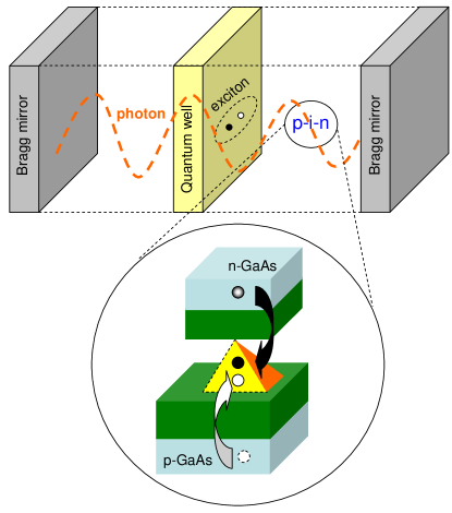
Figure 1: (Color online) Schematic diagram of the system: a semiconductor quantum well is placed between two Bragg mirrors. A quantum dot p-i-n junction is embedded between the well and the mirror to detect the photon part of the polaritons. For simplicity, the substrate of the QDs is not shown.

II Quantum dot p-i-n junction in a microcavity

Consider now a QD p-i-n junction embedded inside a semiconductor microcavity, where the quantum well excitons and cavity photons condense to their ground state as shown in Fig. 1. When this condensation occurs, a great number of polaritons, $\widehat{b}_{\mathbf{k}}$, will occupy the zero-momentum state $\mathbf{k}_{0}$. The canonical transformation^1,2

$$\widehat{b}_{\mathbf{k}}=\sqrt{N^{\prime}}e^{i\phi}\delta_{\mathbf{k},\mathbf{k}_{0}}+\widehat{\alpha}_{\mathbf{k}}$$ (1)

is commonly used to describe $N^{\prime}$ condensed particles and non-condensate particles with operator $\widehat{\alpha}_{\mathbf{k}}$. The polariton operator $\widehat{b}_{\mathbf{k}}$ is composed of the exciton operator, $\widehat{c}_{\mathbf{k}}$, and photon operator, $\widehat{a}_{\mathbf{k}}$,

$$\widehat{b}_{\mathbf{k}}=u_{\mathbf{k}}\widehat{c}_{\mathbf{k}}+v_{\mathbf{k}}\widehat{a}_{\mathbf{k}},$$ (2)

where $u_{\mathbf{k}}$ and $v_{\mathbf{k}}$ are coefficients easily obtained from the diagonalization of exciton-photon interaction¹⁵. From Eq. (2), we can see that there is a one-to-one correspondence of the polariton operator to the photon one. Therefore, the canonical transformation in Eq. (1) can also be applied to the photon operator:

$$\widehat{a}_{\mathbf{k}}=\sqrt{N}e^{i\varphi}\delta_{\mathbf{k},\mathbf{k}_{0}}+\widehat{\beta}_{\mathbf{k}\neq\mathbf{k}_{0}},$$

where $\widehat{\beta}_{\mathbf{k}}$ represents the photons not in the zero momentum state. The photon condensate fraction $N$ is related to $N^{\prime}$ via the particular choice of the diagonalization in Eq. (2).

In this case, the exciton-photon interaction in the QD p-i-n junction, $H_{\mathrm{ex-ph}}$, can now be written as

$$H_{\mathrm{ex-ph}}=T_{0}e^{i\varphi}\left|\uparrow\right\rangle\left\langle\downarrow\right|+\sum_{\mathbf{k}\neq\mathbf{k}_{0}}D_{\mathbf{k}}\left|\uparrow\right\rangle\left\langle\downarrow\right|\widehat{\beta}_{\mathbf{k}}+\text{H.c.},$$ (3)

where $T_{0}=\sqrt{N}D_{\mathbf{k}_{0}}$, with $D_{\mathbf{k}}$ being the coupling strength between the dot exciton and the cavity photon. The index $\mathbf{k}_{0}$ represents the condensate ground state.

We have essentially assumed a mean-field interaction, so that the field of the condensate mode is just represented by a $c$-number: there is no backaction from the QD to the cavity. From the theory of transport through QDs, the first term in Eq. (3) represents coherent tunneling¹⁶, while the second term describes incoherent tunneling¹⁴. Here, we have introduced the three dot states: $\left|0\right\rangle=\left|0,h\right\rangle$, $\left|\uparrow\right\rangle=\left|e,h\right\rangle$, and $\left|\downarrow\right\rangle=\left|0,0\right\rangle$, where $\left|0,h\right\rangle$ means that there is one hole in the QD, $\left|e,h\right\rangle$ is the exciton state, and $\left|0,0\right\rangle$ represents the ground state with no hole and no electron in the QD¹⁴. The Hamiltonian describing the tunneling to the electron and hole reservoirs can thus be written as

$$H_{T}=\sum_{\mathbf{q}}(V_{\mathbf{q}}\widehat{d}_{e,\mathbf{q}}^{\dagger}\left|0\right\rangle\left\langle\uparrow\right|+W_{\mathbf{q}}\widehat{d}_{h,\mathbf{q}}^{\dagger}\left|0\right\rangle\left\langle\downarrow\right|+\text{H.c.}),$$ (4)

where $\widehat{d}_{e,\mathbf{q}}$ and $\widehat{d}_{h,\mathbf{q}}$ are the electron operators in the electron and hole reservoirs, respectively. Here, $V_{\mathbf{q}}$ and $W_{\mathbf{q}}$ couple the channel with momentum $\mathbf{q}$ of the electron and the hole reservoirs.

One can now write the equation of motion for the reduced density operator:

$$\frac{d}{dt}\rho(t) = -i[H_{\mathrm{coh}}(t),\rho(t)]-\mathrm{Tr}_{\mathrm{res}}\int_{0}^{t}dt^{\prime}[H_{\mathrm{incoh}}(t)$$ (5)

$$+H_{T}(t),[H_{\mathrm{incoh}}(t^{\prime})+H_{T}(t^{\prime}),\widetilde{\Xi}(t^{\prime})]],$$

where $\widetilde{\Xi}(t^{\prime})$ is the total density operator, and $H_{\mathrm{coh}}$ ($H_{\mathrm{incoh}}$) represents the coherent (incoherent) tunneling in Eq. (3). Note that the trace, $\mathrm{Tr}$, in Eq. (5) is taken with respect to both the non-condensate photons and the electronic reservoirs.

III Tunneling current

If the couplings to the non-condensate photons and to the electron/hole reservoirs are weak, then it is reasonable to assume that the standard Born-Markov approximation with respect to these couplings is valid. In this case, one can derive a master equation from the exact time-evolution of the system and obtain the tunnel current through the hole-side barrier¹⁴: $I(t)\equiv-e\Gamma_{R}\left\langle\widehat{n}_{\downarrow}\right\rangle_{t}$, where $\widehat{n}_{\downarrow}=\left|\downarrow\right\rangle\left\langle\downarrow\right|$ and $\Gamma_{R}$ is the tunneling rate from the hole side reservoir.

In the steady state limit ($t\rightarrow\infty$), the analytical expression for the tunneling current $I$ is given by

$$I(t\rightarrow\infty)=\frac{2\Gamma_{R}T_{0}^{2}+2\gamma\varepsilon^{2}}{[\varepsilon^{2}+T_{0}^{2}(2+\Gamma_{R}/\Gamma_{L})]+\gamma\varepsilon^{2}(1/\Gamma_{R}+1/\Gamma_{L})},$$ (6)

where $\varepsilon^{2}=E_{0}^{2}+\Gamma_{R}^{2}$. Here, $E_{0}$ is the quantum dot exciton bandgap, $\Gamma_{L}$ is the tunneling rate from the electron-side reservoir, and $\gamma$ is the incoherent decay rate due to the non-condensate photons. Note that, for convenience, we have set the electron charge $e=1$ and Planck constant $\hbar=1$.

Examining Eq. (6) we note that, when the condensation number $N$($\propto T_{0}^{2}$) becomes relatively large, the steady-state current $I(t\rightarrow\infty)$ saturates to the value:

$$I(t\rightarrow\infty)\underset{N\rightarrow\infty}{\longrightarrow}\frac{\Gamma_{R}}{1+\frac{\Gamma_{R}}{2\Gamma_{L}}},$$ (7)

depending only on the values of the tunneling rates $\Gamma_{L}$ and $\Gamma_{R}$. In the opposite limit of no condensation, Eq. (6) is reduced to the result of incoherent case¹⁷:

$$I(t\rightarrow\infty)\underset{T_{0}\rightarrow 0}{\longrightarrow}\left(\frac{1}{\Gamma_{R}}+\frac{1}{\Gamma_{L}}+\frac{1}{\gamma}\right)^{-1}.$$ (8)

The curve in the inset of Fig. 2 shows that the current $I$ increases when increasing the occupation number $N$. Such a phenomenon may be observed by increasing the power of the laser excitation, as has been performed in experiments⁵. Note that in the inset of Fig. 2 and the following figures, we have set the exciton bandgap $E_{0}=1.4$ $\mathrm{eV}$  and the tunneling rates: $\Gamma_{R}=10\Gamma_{L}=0.1$ $\mathrm{meV}$.

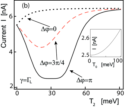
Figure 2: (Color online) Under the influence of two independent condensates, the dotted, red-dashed, and continuous black curves represent the current through the QD p-i-n junction for different values of phase difference: $\varphi_{1}-\varphi_{2}=0$, $3\pi/4$, and $\pi$, respectively. In plotting the figure, the values of $T_{1}$ $(=30\mathrm{meV})$ and incoherent rate $\gamma$ $(\gamma=\Gamma_{L})$ are kept fixed. The inset shows the current increases when increasing the condensation number $N$ ($\propto T_{0}^{2}$) for the case of only a single condensate. $T_{0}$ is the coupling strength between the dot exciton and the cavity photon. 

IV Interference between two condensates

Another important effect that can be examined is the interference between two condensates, which has been observed and verified in dilute atomic gases¹⁸. Consider now an additional quantum well in the microcavity, so that the excitons in this well also form a condensate with the photons. The interactions experienced by the p-i-n junction experiences can be described by

$$H_{\mathrm{2ex-ph}}=\sum_{j=1,2}\{T_{j}e^{i\varphi_{j}}\left|\uparrow\right\rangle\left\langle\downarrow\right|+\sum_{\mathbf{k}\neq\mathbf{k}_{0}}D_{j,\mathbf{k}}\left|\uparrow\right\rangle\left\langle\downarrow\right|\widehat{\beta}_{j,\mathbf{k}}\}+\text{H.c.},$$ (9)

where the two phases $\varphi_{1}$ and $\varphi_{2}$ come from the $U(1)$ symmetry-breaking of the two condensates. Assuming that the exciton-photon couplings of the two wells are identical, the coherent parts, $T_{j}=\sqrt{N_{j}}D_{\mathbf{k}_{0}}$, contain the information of the excitation numbers $N_{1}$ and $N_{2}$. The resultant steady-state current is similar to Eq. (6), besides the following replacement:

$$T_{0}^{2}\rightarrow D_{\mathbf{k}_{0}}^{2}[N_{1}+2\sqrt{N_{1}N_{2}}\cos(\varphi_{1}-\varphi_{2})+N_{2}].$$ (10)

For a fixed $N_{1}$, the dotted, red-dashed, and black curves in Fig. 1(b) represent the steady-state currents as functions of $N_{2}$, for the phase differences $\varphi_{1}-\varphi_{2}=0$, $3\pi/4$, and $\pi$, respectively. As seen in Fig. 2, the dips in the currents reveal the effect of destructive interference when $\varphi_{1}-\varphi_{2}$ approaches $\pi$.

We also suggest that the p-i-n junction can be embedded inside an array of polariton condensates connected by weak periodic potential barriers⁶, where the in-phase (‘zero-state’) and anti-phase (‘$\pi$-state’) have been created. In this case, Eqs. (6) and (10) can also be used to distinguish the zero-state and $\pi$-state.

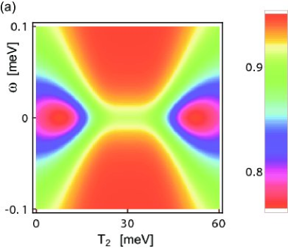
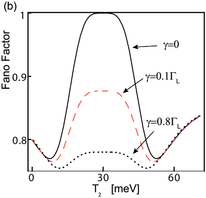
Figure 3: (Color online) (a) Shot-noise spectra of a QD p-i-n junction as functions of both $\omega$ and the coupling $T_{2}$ to the 2^nd condensate. Here, the excitons are coupled to two condensates. Similar to Fig. 1(b), one of the condensate numbers is kept fixed, i.e. $T_{1}=30$ $\mathrm{meV}$. (b) By fixing the phase difference $\varphi_{1}-\varphi_{2}=\pi$, the continuous black, red dashed, and dotted curves represent the Fano factor (zero-frequency noise) for $\gamma=0$, $0.1\Gamma_{L}$, and $0.8\Gamma_{L}$, respectively. The Fano factor is defined here as $S_{I_{R}}(\omega\rightarrow 0)/2eI$.

V Shot-noise measurements

Recently, interest in measurements of shot-noise in quantum transport has grown owing to the possibility of extracting valuable information not available in conventional dc transport experiments¹⁹. Therefore, in addition to the current, we now proceed to calculate the noise spectrum.

In a quantum conductor out of equilibrium, electronic current-noise originates from the dynamical fluctuations of the current away from its average. To study correlations between carriers, we relate the exciton dynamics with the hole reservoir operators by introducing the degree of freedom $n$ as the number of holes that have tunneled through the barrier connected to the reservoir of holes and write

$$\overset{\cdot}{n}_{0}^{(n)}(t) = -\Gamma_{L}n_{0}^{(n)}(t)+\Gamma_{R}n_{\downarrow}^{(n-1)}(t),$$ (11)

$$\overset{\cdot}{n}_{\uparrow}^{(n)}(t) = \Gamma_{L}n_{0}^{(n)}(t)+iT[p_{\uparrow,\downarrow}^{(n)}(t)-p_{\downarrow,\uparrow}^{(n)}(t)]-\gamma n_{\uparrow}^{(n)}(t),$$

$$\overset{\cdot}{n}_{\downarrow}^{(n)}(t) = -\Gamma_{R}n_{0}^{(n)}(t)-iT[p_{\uparrow,\downarrow}^{(n)}(t)-p_{\downarrow,\uparrow}^{(n)}(t)]+\gamma n_{\uparrow}^{(n)}(t),$$

where $n_{j}^{(n)}(t),$ $j=$ $0$, $\uparrow,$ $\downarrow$, represent the time-dependent occupation probabilities for the diagonal elements: $\left|0\right\rangle\left\langle 0\right|$, $\left|\uparrow\right\rangle\left\langle\uparrow\right|$, and $\left|\downarrow\right\rangle\left\langle\downarrow\right|$, respectively. Here, $p_{\uparrow,\downarrow}(t)$ and $p_{\downarrow,\uparrow}(t)$ are the off-diagonal matrix elements: $\left|\uparrow\right\rangle\left\langle\downarrow\right|$ and $\left|\uparrow\right\rangle\left\langle\downarrow\right|$. $T$ is the “coherent” interaction that the dot experiences. The superscript ‘$n$’ in $n_{j}^{(n)}(t)$ refers to the $n$ holes that have tunneled the barrier connecting to the hole reservoir.

The Eqs. (11) allow us to calculate the particle current and the noise spectrum $S_{I_{R}}(\omega)$ from $P_{n}(t)=n_{0}^{(n)}(t)+n_{\uparrow}^{(n)}(t)+n_{\downarrow}^{(n)}(t)$ which gives the total probability of finding $n$ electrons in the collector at time $t$. In particular, the noise spectrum $S_{I_{R}}$ can be calculated via the MacDonald formula²⁰

$$S_{I_{R}}(\omega)=2\omega e^{2}\int_{0}^{\infty}dt\sin(\omega t)\frac{d}{dt}[\left\langle n^{2}(t)\right\rangle-(t\left\langle I\right\rangle)^{2}],$$ (12)

where $\frac{d}{dt}\left\langle n^{2}(t)\right\rangle=\sum_{n}n^{2}\overset{\cdot}{P_{n}}(t)$. From Eqs. (11) and (12), we obtain

$$S_{I_{R}}(\omega)=2eI\{1+\Gamma_{R}[\widetilde{n}_{\downarrow}(-i\omega)+\widetilde{n}_{\downarrow}(i\omega)]\},$$ (13)

where $\widetilde{n}_{\downarrow}(z)$ is the Laplace transformation of $n_{\downarrow}(t)$.

By fixing $T_{1}=30$ meV and $\varphi_{1}-\varphi_{2}=\pi$, an interference effect can be observed in the noise spectrum as a function of $T_{2}$ and $\omega$, as shown in Fig. 3(a). The figure shows two symmetric lobes around $T_{2}=T_{1}$, which represent the local minima. To understand these features, we plot in Fig. 3(b) the Fano factor (i.e., the zero-frequency noise divided by the current) as a function of $T_{2}$ for different values of the incoherent decay rate $\gamma$. One clearly finds that the magnitude of the central peak decreases when increasing $\gamma$. As the incoherent process dominates due to the non-condensate photons overwhelming the coherent ones, therefore the Fano factor reduces to the usual sub-Poissonian limit²¹. In the opposite limit ($\gamma\rightarrow 0$), the Fano factor approaches unity, i.e. the Poissonian value, demonstrating that the revealing feature of destructive interference is a peak in the Fano factor (at $\omega=0$), coinciding with the dip in the steady-state current observed in Fig. 1(b).

VI Concluding remarks

An alternative way to detect the condensation of polaritons via electron transport is by directly embedding the quantum well between a p-n junction. We expect that in this case the increase of the steady-state current with the condensation number $N$ might be observable. However, the features we observed in the current-noise spectrum may be invisible since the assumption of three dot states is not valid in a quantum well.

In summary, we have shown that a single QD p-i-n junction can serve as a mini-detector²² inside the quantum structure, such that the features of condensation and interference can be readout via the electrical current and current-noise.

- (1) L. D. Landau and E.M. Lifshitz, Statistical Physics (Pergamon, London, 1969).
- (2) See, e.g., L. P. Pitaevskii and S. Stringari, Bose-Einstein Condensation (Clarendon, Oxford, 2003).
- (3) S. A. Moskalen, Sov. Phys. Solid State 4, 199 (1962); J. M. Blatt, Phys. Rev. 126, 1691 (1962); L. V. Keldysh and A. N. Kozlov, Sov. Phys. JETP 27, 521 (1968).
- (4) For a review see, e.g., D. W. Snoke, Phys. Status. Solidi B 238, 389 (2003).
- (5) J. Kasprzak, M. Richard, S. Kundermann, A. Baas, P. Jeambrun, J. M. J. Keeling, F. M. Marchetti, M. H. Szymaska, R. Andre, J. L. Staehli, V. Savona, P. B. Littlewood, B. Deveaud and Le Si Dang, Nature 443, 409 (2006).
- (6) C. W. Lai, N. Y. Kim, S. Utsunomiya, G. Roumpos, H. Deng, M. D. Fraser, T. Byrnes, P. Recher, N. Kumada, T. Fujisawa and Y. Yamamoto, Nature 450, 529 (2007).
- (7) K. G. Lagoudakis, M. Wouters, M. Richard, A. Baas, I. Carusotto, R. Andre, Le Si Dang and B. Deveaud-Pledran, Nature Physics 4, 706 (2008).
- (8) S. Utsunomiya, L. Tian, G. Roumpos, C. W. Lai, N. Kumada, T. Fujisawa, M. Kuwata-Gonokami, A. Loffler, S. Hofling, A. Forchel and Y. Yamamoto, Nature Physics 4, 700 (2008).
- (9) A. Amo, D. Sanvitto, F. P. Laussy, D. Ballarini, E. del Valle, M. D. Martin, A. Lemaitre, J. Bloch, D. N. Krizhanovskii, M. S. Skolnick, C. Tejedor and L. Vina, Nature 457, 291 (2009).
- (10) See, e. g., C. Cohen-Tannoudji, J. Dupont-Roc, and G. Grynberg, Atom-Photon Interactions: Basic Processes and Applications (Wiley-Interscience, 1992).
- (11) J. P. Reithmaier, G. Sek, A. Loffler, C. Hofmann, S. Kuhn, S. Reitzenstein, L. V. Keldysh, V. D. Kulakovskii, T. L. Reinecke and A. Forchel, Nature 432, 197 (2004); E. Peter, P. Senellart, D. Martrou1, A. Lemaitre, J. Hours, J. M. Gerard, and J. Bloch, Phys. Rev. Lett. 95, 067401 (2005).
- (12) T. Yoshie, A. Scherer, J. Hendrickson, G. Khitrova, H. M. Gibbs, G. Rupper, C. Ell, O. B. Shchekin and D. G. Deppe, Nature 432, 200 (2004); K. Hennessy, A. Badolato, M. Winger, D. Gerace, M. Atature, S. Gulde, S. Falt, E. L. Hu and A. Imamoglu, Nature 445, 896 (2007).
- (13) Z. Yuan, B. E. Kardynal, R.M. Stevenson, A. J. Shields, C. J. Lobo, K. Cooper, N. S. Beattie, D. A. Ritchie, and M. Pepper, Science 295, 102 (2002).
- (14) See, e.g., Y. N. Chen, D. S. Chuu, and T. Brandes, Phys. Rev. Lett. 90, 166802 (2003).
- (15) S. A. Moskalenko and D. W. Snoke, Bose-Einstein Condensation of Excitons and Biexcitons (Cambridge University Press, Cambridge 2000).
- (16) R. Aguado and T. Brandes, Phys. Rev. Lett. 92, 206601 (2004); N. Lambert and F. Nori, Phys. Rev. B 78, 214302 (2008).
- (17) Y. N. Chen and D. S. Chuu, Phys. Rev. B 66, 165316 (2002).
- (18) M. R. Andrews, C. G. Townsend, H.-J. Miesner, D. S. Durfee, D. M. Kurn, W. Ketterle, Science 275, 637 (1997).
- (19) See, e.g., C. W. J. Beenakker, Rev. Mod. Phys. 69, 731 (1997); Y. M. Blanter and M. Buttiker, Phys. Rep. 336, 1 (2000).
- (20) D. K. C. MacDonald, Rep. Prog. Phys. 12, 56 (1948).
- (21) Y. N. Chen, T. Brandes, C. M. Li, and D. S. Chuu, Phys. Rev. B 69, 245323 (2004).
- (22) P. Neutens, P. V. Dorpe, I. D. Vlaminck, L. Lagae, and G. Borghs, Nature Photonics 3, 283 (2009).