Kondo effect in a side-coupled double-quantum-dot system embedded in a mesoscopic ring

Abstract

We study the finite size effect of the Kondo screening cloud in a double-quantum-dot setup via a large-N slave-boson mean-field theory. In this setup, one of the dots is embedded in a close metallic ring with a finite size $L$ and the other dot is side-coupled to the embedded dot via an anti-ferromagnetic spin-spin exchange coupling with the strength $K$. The antiferromagnetic coupling favors the local spin-singlet and suppresses the Kondo screening. The effective Kondo temperature $T_{k}$ (proptotional to the inverse of the Kondo screening cloud size) shows the Kosterlitz–Thouless (KT) scaling at finite sizes, indicating the quantum transition of the KT type between the Kondo screened phase for $K\leq K_{c}$ and the local spin-singlet phase for $K\geq K_{c}$ in the thermodynamic limit with $K_{c}$ being the critical value. The mean-field phase diagram as a function of $1/L$ and $K$ shows a crossover between Kondo and local spin-singlet ground states for $K<K_{c}$ ($L=4n,4n+1,4n+3$) and for $K>K_{c}$ ($L=4n+2$). To look into the crossover region more closely, the local density of states on the quantum dot and the persistent current at finite sizes with different values of $K$ are also calculated.

.1 I. Introduction

Kondo effectHewson , the screening of magnetic impurities by the conduction electron reservoir, has been intensively studied over the last half-century. Recently, there has been revival interest in Kondo effect in semiconductor quantum dot devices due to the progress in fabracating nanostructuresgoldharber . When there are odd number of electrons on the dot, Kondo effect overcomes the Coulomb Blockade, leading to a narrow pronounced resonance peak in local impurity density of states and enhanced conductance through the quantum dotglazman goldharber . The Kondo effect is characterized by the single energy scale , the Kondo temperature $T_{k}\approx De^{-1/J}$Hewson , below which the Kondo screening develops. Here, $D$, $J$ in $T_{k}$ are the conduction electron bandwidth and the dimensionless Kondo coupling, respectively. In a finite-sized mesoscopic device, $T_{k}$ sets the length scale $\xi_{k}^{0}\approx\hbar v_{F}/T_{k}$ associated with the size of the Kondo screening cloud where the cloud of electrons with the size of order of $\xi_{k}^{0}$ surrounding the magnetic impurity form spin-singlet state with itring1 . Here, $v_{F}$ is the Fermi velocity. For typical values of $T_{k}$, $\xi_{k}^{0}$ is around $0.1~{}1\mu m$, which is comparable to the typical size of the quantum dot device, leading to the finite size effect of the Kondo screening cloud. This effect has been investigated in a quantum dot embedded in a mesoscopic ring threaded by a magnetic fieldring1 ring2 ring3 . The experimentally measurable persistent current induced by the magnetic flux has been shown to be sensitive to the ratio of the size of the ring $L$ and $\xi_{k}^{0}$ ring1 ring2 ring3 . As $L\ll\xi_{K}^{0}$ the Kondo screening cloud does not develop completely, giving rise to the suppression of Kondo effect and a reduction of the persistent current even if the temperature is lower than $T_{k}$; while as for $L\gg\xi_{k}^{0}$ the Kondo screening cloud is formed, leading to enhanced persistent current. By measuring the transport properties (such as: persistent current) as a function of the system size, we gain insights on how the Kondo screening cloud is formed as the system size is increased. This idea offers another route to realize Wilson’s Numerical Renormalization Group (NRG)NRG idea on the Kondo problem.

Very recently, study of the Kondo effect has been extended to the coupled double-quantum-dot setups via antiferromagnetic RKKY interactionsMarcus2QD chung2QD rkkyPascal cornaglia . The Kondo effect in such double-dot systems competes with the RKKY interactions, giving rise to quantum phase transition in the context of the well-known two-impurity Kondo problem between the Kondo and local spin-singlet ground states2impkondo . Close to the quantum critical point physical observables at finite temperatures exhibit non-Fermi liquid behaviors. The crossover behaviors between these two phases can be accessed by changing temperatures. However, at zero temperature but at finite-sizes, the size of the Kondo screening cloud provides us with an alternative route to the crossover behaviors in the two-impurity Kondo problempascal .

In this paper, we study the Kondo effect in a side-coupled double quantum dot system embedded in a finite-sized mesoscopic ring. A similar side-coupled double-quantum-dot system has been studied where one of the dot is coupled to Fermi-liquid leads of conduction electrons with continuous spectrumside-coupled . Unlike the two-impurity Kondo system, in the side-coupled double-dot system the Kondo phase is fragile and unstable towards the local spin-singlet state for any infinitesmall antiferromagnetic spin-exchange coupling, and the transition is of the Kosterliz-Thouless type. Note that a related setup consisting of double quantum dots in parallel connected to a mesoscopic ring shows a quantum phase transition of the pseudogap Anderson model when the magnetic flux is tuneddias . Here, we are interested in not only the nature of the Kondo-to-spin-singlet quantum phase transition in our proposed setup but also the crossover phenomena via a systematic study of the system at finite sizes. The inverse of the system size $1/L$ plays a similar role as temperature $T$. The finite temperature crossover behaviors between the above two quantum ground states can therefore be accessed effectively via changing the size of the ring.

We focus on the following three quantities to investigate this issue: the effective Kondo temperature $T_{k}$ (inversely proportional to the size of the Kondo screening cloud $\xi_{k}$ in the presence of the antiferromagnetic spin exchange coupling), the local density of states (DOS) $\rho_{QD}(\omega)$ on the quantum dot, and the persistent current (PC) $I$. The plan of the paper is as follows. In Section II., we introduce the model and present a large-N mean-field treatment of the model. In Section III., we present our results on the effective Kondo temperature, the local DOS on the dot and the persistent current. We also give detail explanations of our results. The conclusions are given in Section IV..

Figure 1: Sketch of the model. $t_{L}/t_{R}$ is the hopping coefficient between dot $1$ and its left/right conducting island on the ring, $\phi$ is the magnetic flux (in unit of $2\pi/\Phi_{0}$ with $\Phi_{0}=hc/e$) through the ring, $K$ is antiferromagnetic coupling between dot $1$ and dot $2$.

.2 II. Model

Our model describes a double-quantum-dot system embedded in electronic reservoir in a finite-sized ring (see Fig.1). In this setup, only one of the dot (dot $1$) is coupled to the ring via hoping; while the other dot (dot $2$) is coupled only to dot $1$ via antiferromagnetic spin-exchange interaction with a coupling strength $K$ and is decoupled from the reservoir of the ring. The ring serves as electronic reservoir consists of $L-1$ conducting islands. We consider here the half-filled case ($N_{e}=L+1$ where $N_{e}$ is the total number of electrons on the ring and on the two dots). The key point in this setup with a closed geometry is that the Kondo screening cloud is trapped in the ring and can not escape into the external leadsring1 . Nevertheless, one can measure the transmission probability through the quantum dot $1$ embedded in the ring by measuring the persistent currentring1 Buttiker (see details in Sec. III.). Here we assume a direct antiferromagnetic spin exchange coupling between two quantum dots which competes with the Kondo effect. Note that though it has been known experimentally that the antiferromagnetic spin-spin coupling (RKKY interaction) between a double-quantum-dot system can be induced naturally by a conduction electron island in the middle of the two dotsMarcus2QD , the direct antiferromagnetic spin exchange coupling may in principle be generated via the second-order hoping process directly between the two dots if the two quantum dots are close enough to each other. Since in both cases we expect suppression of the Kondo effect due to local spin-spin exchange coupling, to simplify our calculations we assume a direct antiferromagnetic spin-exchange coupling between the two dots.

The Hamiltonian of our model is given by:

$${H} =H_{A}+KS_{1}\cdot S_{2}$$ (1)

where $H_{A}$ represents a quantum dot embedded in a ring by the Anderson impurity model.

$${H}_{A} = -t\sum_{j=1}^{L-1}\sum_{\sigma}[c_{j}^{\dagger}c_{j+1}+H.C]+U\sum_{i=1,2}n_{d_{i}}^{\uparrow}n_{d_{i}}^{\downarrow}+\sum_{\sigma,i=1,2}\epsilon_{d}d_{i\sigma}^{\dagger}d_{i\sigma}$$

$$- \sum_{\sigma}[t_{L}d_{1\sigma}^{\dagger}c_{1\sigma}+t_{R}\exp(i\phi)c_{L-1\sigma}^{\dagger}d_{1\sigma}+H.c.]$$

where $c_{j}$, $d_{1}$, $d_{2}$ represent the annihilation operators of electron on site $j$ of the ring, dot $1$ and dot $2$, respectively, the phase factor $\phi$ is defined by $\phi=2\pi\Phi/\Phi_{0}$ with $\Phi$ being the magnetic flux going through the ring and $\Phi_{0}=hc/e$ being the flux quantum, $t$ is the electron hoping within the tight-binding ring, and $t_{L/R}$ are the hopings between dot $1$ and the two neighboring ring electrons ($c_{L-1}$/$c_{1}$). Here, $S_{1}$ and $S_{2}$ represent spin operators of dot $1$ and dot $2$, respectively with $S_{i}=\sum_{\sigma\sigma^{\prime}}d_{i\sigma}^{\dagger}\sigma_{\sigma\sigma^{\prime}}d_{i\sigma^{\prime}}$. $L$ is the total number of electrons in the system excluding dot $2$. The well-known Kondo limit is reached for $U\gg t$. Here, we consider a simple limit in the Kondo regime, $U\rightarrow\infty$ where the slave-boson mean-field (SBMF) approachring2 ring3 is applicable to simplify the quartic $U$ term.

Further progress can be made by decoupling the quartic spin-spin interaction $S_{1}\cdot S_{2}$ into qudratic one via the Hubbard-Stratonovish transformation in the framework of the large-N $SU(N)$ mean-field theory where the symmetry of the Hamiltonian is generalized from the $SU(2)$ with spin degeneracy being two to $SU(N)$ with spin degeneracy being $N\rightarrow\infty$Hewson . In the SU(N) generalization of the slave-boson representation, we have $d_{i\alpha}$ = $f_{i\alpha}b_{i}^{\dagger}$, $\alpha$ is the flavor of the spin: $\alpha=1,2,...N$, $i=1,2$ is the indix for the two quantum dots. The local constraints to enforce the single occupancy on dot $1$ and $2$ are given by

$$\sum_{\alpha}f_{i}^{\dagger\alpha}f_{i\alpha}+b_{i}^{\dagger}b_{i}=\frac{N}{2}$$ (3)

The mean-field Hamiltonian for $H_{A}$ is therefore given by,

$$NH_{A,MF} = -t\sum_{j=1}^{L-1}\sum_{\alpha=1}^{N}[c_{j\alpha}^{\dagger}c_{j+1\alpha}+H.c.]+\sum_{\alpha=1}^{N}\widetilde{\epsilon_{d}}f_{1\alpha}^{\dagger}f_{1\alpha}+\sum_{\alpha=1}^{N}\epsilon_{d}^{\prime}f_{2\alpha}^{\dagger}f_{2\alpha}$$

$$- \sum_{\alpha=1}^{N}[\widetilde{t_{L}}f_{1\alpha}^{\dagger}c_{1\alpha}+\widetilde{t_{R}}\exp(i\phi)c_{L-1\alpha}^{\dagger}f_{1\alpha}+H.c]+\lambda(b_{0}^{2}-1)+\bar{\lambda}(\bar{b}^{2}-1)$$

where $\widetilde{t}_{L/R}=b_{0}t_{L/R}$ with $b_{0}$ being the expectation value of the $b_{1}$ boson on dot $1$, $b_{0}=<b_{1}>$, $\bar{b}=<b_{2}>$, $\lambda$ ($\bar{\lambda}$) is the Lagrange multiplier which enforces the local contraint on dot $1$ ($2$), $\tilde{\epsilon_{d}}=\epsilon_{d}-\lambda$, $\epsilon_{d}^{\prime}=\epsilon_{d}-\bar{\lambda}$. The quartic antiferromagnetic spin-spin interaction can be decoupled via the mean-field variable $\chi$ chung-largeN :

$$\chi=\frac{b_{0}K}{N}<d_{1}^{\dagger\alpha}d_{2,\alpha}>$$ (5)

. Therefore,

$$KS_{1}\cdot S_{2} = -\sum_{\alpha=1}^{N}\frac{\chi}{N}f_{1}^{\dagger\alpha}f_{2\alpha}-H.c.+\frac{\chi^{2}}{K}$$ (6)

The full mean-field Hamiltonian is given by

$$H_{MF}=H_{A,MF}-\sum_{\alpha=1}^{N}\frac{\chi}{N}f_{1}^{\dagger\alpha}f_{2\alpha}-H.c.+\frac{\chi^{2}}{K}.$$ (7)

The mean-field energy $E_{MF}$ can be obtained by diagonalizing the above Hamiltonian and can be expressed as

$$E_{MF}=\sum_{m,\sigma}\epsilon_{m,\sigma}(\lambda,b_{0})+\frac{\chi^{2}}{K}+\lambda(b_{0}^{2}-1)+\bar{\lambda}(\bar{b}^{2}-1),$$ (8)

where $\epsilon_{m,\sigma}$ are the eigenvalues of the Hamiltonian matrix in $H_{MF}$, the summation over m includes all occupied levels of $H_{MF}$. The values of the mean-field variables $\lambda$, $b_{0}$ and $\chi$ are determined by minimizing $E_{MF}$ with respect to $b_{0}$ and $\chi$:

$$\frac{\partial E_{MF}}{\partial b_{0}}=\frac{\partial E_{MF}}{\partial\bar{b}}=\frac{\partial E_{MF}}{\partial\chi}=0,$$ (9)

subject to the constraint $\frac{\partial E_{MF}}{\partial\lambda}=\frac{\partial E_{MF}}{\partial\bar{\lambda}}=0$. The ground state energy $E_{gs}$ corresponds to the global minimum of $E_{MF}(\lambda,\bar{\lambda},b_{0},\bar{b},\chi)$ which satisfies the mean-field equations. Note that the advantages of taking the large-$N$ mean-field approach are: (i) in the large-$N$ limit the solutions from the mean-field equations are exact though the physical system corresponds to $N=2$, and (ii) at finite $N$, a systematic $1/N$ correction to the mean-field results is possible though it is beyond the scope of this paper. The mean-field phase diagram can be mapped out via the solutions of the above mean-field equations.

Figure 2: Schematic mean-field phase diagram of the model for (a) $L=4n,4n+1,4n+3$ (case (I)) and (b) $L=4n+2$ (case (II)). The red line indicates the crossover with $K$ being fixed and the green line indicates the crossover with $L$ being fixed.

.3 III. Results

Three physical observables are identified to investigate the Kondo screening effect of our setup at finite sizes: (i). Effective Kondo temperature($T_{k}$), (ii). Local density of states on dot $1$ (LDOS) ($\rho_{QD}(\omega)$), (iii). Persistent current(PC). Details are shown below.

Before we present our new results, it is useful to summarize the behavior of the model at $K=0$ (without antiferromagnetic spin-spin coupling), which has been intensively studiedring1 ring2 ring3 . The Kondo resonance of a quantum dot embedded in a mesoscopic ring strongly depends on the finite size $L$ (mod $4$), and the magnetic flux $\Phi$ threading the ring. In particular, both the Kondo temperature $T_{k}$ and the persistent current $I$ follow universal scaling functions of $\xi_{k}^{0}/L$ at a fixed magnetic flux. In the Kondo regime, all physical observables, such as: Kondo temperature $T_{k}$, persistent current $I$ are enhanced as the size $L$ increases, but with different crossover bahaviors in all four cases of $L=4n$, $L=4n+1$, $L=4n+2$, and $L=4n+3$. The magnetic flux dependence of persistent current $I$ exhibits a symmetry between size $L$ and $L+2$: $I_{L}(\phi)=I_{L+2}(\phi+\pi)$, indicating that adding the magnetic flux of $\Phi_{0}/2$ (or adding a phase $\pi$) is equivalent to switch the behavior of the PC from a system with size $L$ to $L+2$.

With the previous results in mind, we may discuss the general properties for $K>0$. Due to the antiferromagnetic spin-spin couping, we expect in this case the competition between the Kondo and the local spin-singlet ground states, leading to the quantum phase transition. In fact, quantum phase transitions in double-quantum-dot systems with antiferromagnetic RKKY interactions have been intensively studied in recent years Marcus2QD chung2QD in the framework of two-impurity Kondo problem 2impkondo where the quantum dots couple to the conduction electron Fermi sea with continuous spectrum. Two types of quantum phase transitions have been identified in these systems: the phase transition with a quantum critical point (QCP) and the one of the Kosterlitz-Thouless (KT) type. The characteristic behavior near QCP is the observables power-law dependence on the coupling strength relative to the critical point; while for the KT transition the crossover energy scale exponentially depend on the distance to the critical point. The former (QCP) type of the quantum phase transition is realized in the double-dot systems where each of the dot couples to an independent conduction electron reservoirMarcus2QD chung2QD , and the critical point separating the Kondo from the local spin-singlet phase is the well-known two-impurity Kondo fixed point2impkondo . The latter (KT) type exsits in a side-coupled double-dot system where only one of the dots coupled to the electron reservoirside-coupled . The Kondo resonance becomes more fragile in the side-coupled system so that an infinitesmall antiferromagnetic coupling is sufficient to suppress the Kondo effect and leads to the spin-singlet ground state. We expect the similar Kosterlitz-Thouless transition to occur in our side-coupled double-dot system embedded in a ring. However, the mesoscopic ring in our setup consists of a finite number of tight-binding electrons (instead of a Fermi sea with continuous spectrum), the details of the transition might be different from those in Ref.side-coupled (see below).

.3.1 A. Mean-field phase diagram

After solving the mean-field equations, we summarize our main results in the schematic mean-field phase diagram as shown in Fig. 2. We find indeed the transition between the Kondo and spin-singlet phases is of the Kosterlitz-Thouless type (see below). However, we find that the critical point $K_{c}$ separating the two phases is not at zero as shown in the similar side-coupled double-dot system studied previously in Ref.  side-coupled but at a finite value: $K_{c}>0$.

There are three regions in the phase diagram, corresponding to different mean-field solutions:

1. For small $K$ we find $b_{0}\neq 0$, $\lambda\neq 0$, $\chi=0$. In the thermodynamic limit this is the Kondo phase studied in Ref.ring1 ring2 ring3 .

2. For large $K$, we find $b_{0}=0$, $\lambda\neq 0$. The ground state for $L\rightarrow\infty$ is the local spin-singlet phase where antiferromagnetic spin-spin coupling completely suppresses the Kondo effect.

3. In the intermediate values of $K$, we find $b_{0}=0$, $\lambda\neq 0$, $\chi\neq 0$. This corresponds to the crossover region between Kondo and spin-singlet phases indicated in the shaded region in Fig.2. This region is defined either by $K_{c1}<K<K_{c2}$ for a fixed size $L$ where $K_{c1}$ and $K_{c2}$ are the boundaries between the crossover region and the two stable phases or by $L_{c1}<L<L_{c2}$ for a fixed $K$ where $L_{c1}$ and $L_{c2}$ are defined in a similar way as $K_{c1}$ and $K_{c2}$.

Note that in all the above three cases, we find $\bar{b}=0$, $\bar{\lambda}=\epsilon_{d}$. We then systematically investigate the crossover behaviors along the following two different crossover paths, depending on the finite size $L$ (mod $4$):

Case (I) (Fig.2 (a)) holds for $L=4n,4n+1,4n+3$ where we find the crossover occurs for $K<K_{c}$.

Case (II) (Fig.2 (b)) occurs for $L=4n+2$ where we find the crossover ranges exist mainly for $K>K_{c}$.

In both cases, we find the crossover energy scale $T^{*}$ follows the behavior of the typical Kosterlitz-Thouless transition:

$$T^{*}=c\widetilde{T_{k}}\exp{[-\pi\widetilde{T_{k}}/(K-K_{c})]}$$ (10)

where $\widetilde{T_{k}}=c^{\prime}T_{k}$, and both $c$ and $c^{\prime}$ are non-universal constants.

We investigate the Kondo effect in our setup at finite sizes by either changing the size $L$ at a fixed $K$ (or following the red (vertical) line in Fig.2) or changing $K$ at a fixed size $L$ (or following the green (horizontal) line in Fig. 2). The finite size scaling of $T_{k}$ indicates that in the thermodynamic limit $L\rightarrow\infty$, $K_{c1}$ and $K_{c2}$ converge to a single critical value $K_{c}$: $K_{c1}=K_{c2}\rightarrow K_{c}$ (see below).

.3.2 B. The effective Kondo temperature

In the single Kondo dot system embedded in a 2D electron gas (2DEG), it is well-known that the physical properties follow universal functions of $(T/T_{K}^{0})$ in Kondo regime where $T_{k}^{0}$ is the Kondo temperature of the single dot in the thermodynamic limitgoldharber . In a single quantum dot embedded in a mesoscopic ring with a finite size, the effective Kondo temperature can be defined asring2

$$T_{k}^{1QD}=\epsilon_{d}-(E_{gs}-E_{gs}^{o})$$ (11)

, where $\epsilon_{d}$ is the energy of the dot $1$, $E_{gs}$ and $E_{gs}^{0}$ correspond to the energy of the full system and of the tight-binding ring with the open boundary condition, respectively. The effective Kondo temperature $T_{k}$ is the energy gain due to the coupling between quantum dot and the ring, which corresponds to the energy associated with the Kondo coupling. In the thermodynamic limit ($L\rightarrow\infty$), $T_{k}$ approaches to $T_{k}^{0}$. For the relevant parameters in the $K=0$ Anderson model of the single dot-ring setup: $t=1$, $t_{L}=t_{R}=0.4t$, $\epsilon_{d}=-0.8t$, we find $T_{k}^{0}\approx 0.0189t$, $\xi_{k}^{0}\sim 106$. Note that for simplicity, we set $t=1$ throughout the paper as our unit.

In the presence of the antiferromagnetic spin-spin coupling the effective Kondo temperature $T_{k}$ at a finite size in the context of our large-N slave-boson mean-field approach can be generalized from Eq. 11 to:

$$T_{k}=\epsilon_{d}-(E_{gs}-E_{gs}^{o})-\frac{\chi^{2}}{K}$$ (12)

Note that the effective $T_{k}$ defined in Eq.11 and Eq.12 are slightly different from that defined in Ref.ring2 where $T_{k}$ is measured relative to the hightest occupied level defined as $\epsilon_{F}$, corresponding to the Fermi energy in the thermodynamic limitring2 ring3 . Though this minor difference in definition does not affect the results and the physics, $T_{k}$ defined here offers an intuitive understanding of the crossover at finite sizes corresponding to case (I) and (II) mentioned above–for $K<K_{c}$, $T_{k}$ is expected to increase with increasing size $L$ for case (I) as the system recovers the Kondo resonance in $L\infty$ limit, and for $K>K_{c}$ $T_{k}$ is expected to decrease to $0$ as the system approaches to the local spin-singlet ground state in the thermodynamic limit (see details below). Nevertheless, we have checked that with the definition in Ref. ring2 and ring3 our results for $T_{k}$ at finite sizes indeed reproduce those in Ref.ring2 and ring3 . We have also checked that our results on $T_{k}$ for $K=0$ are consistent with the finite-size behaviors in $E_{gs}$ and $E_{gs}^{0}$ via perturbation theory in Ref. ring1 .

In the Kondo phase, $T_{k}$ reduces to the Kondo temperature for the single quantum dot embedded in a mesoscopic ring ($K=0$). When $L\rightarrow\infty$, $T_{k}$ in the Kondo phase approaches to $T_{K}^{0}$. In the crossover between Kondo and the local singlet phases, $T_{k}$ decreases with increasing $K$, and finally $T_{k}\rightarrow 0$ when the system is in the local singlet ground state where the Kondo effect is completely suppressed by the antiferromagnetic spin-spin couping. We analysize below in details the crossover between the Kondo and the local spin-singlet ground states from the behaviors of the Kondo temperature.

.3.3 1. Varies K with fixed L

Figure 3: $T_{k}$ as functions of $K$. (a)Case I: $L=4n$ (b)Case II: $L=4n+2$. Other parameters: $\epsilon_{d}$ = -0.8t, $t_{R}$ = $t_{L}$ = 0.4t, $\phi=0$. Here we set $t=1$ as the unit.

We first monitor how the Kondo resonance is destroyed by varying the antiferromagnetic spin-spin coupling strength $K$ at a fixed finite size $L$. Fig.(3) shows $T_{k}$ as a function of antiferromagnetic coupling strength $K$ at a fixed size $L=300$ (or $\xi_{k}^{0}/L\sim 0.3$). In both case (I) and (II), $T_{k}$ vanishes as $K\rightarrow K_{c2}$, indicating the suppression of Kondo resonance by the antiferromagnetic spin-spin interaction. However, there are minor differences between these two cases in how fast $T_{k}$ vanishes as $K$ close to $K_{c2}$. In case (II), $T_{k}$ remains a constant over a wider range of $K<K_{c1}$ compared to that in case (I) before it decays. This suggests that the Kondo effect at a finite size seems more robust in case (II) ($L=4n+2$) than in case (I) ($L=4n,4n+1,4n+3$) so that the crossover region in case (II) is much narrower than in that in case (I). This is consistent with our numerics as $T_{k}$ for $L=4n+2$ is found to have the largest value among $L$ (mod $4$) for a given size.

.3.4 2. Varies $L$ with fixed $K$

Next, we present the results on the finite-size dependence of the Kondo resonance at a fixed antiferromagnetic spin-spin coupling strength $K$. In analogous to the Numerical Renormalization Group (NRG) method, the ground state is computed and monitored as we decrease the energy scale $1/L$ (or equivalently increase the system size $L$) until we reach the thermodynamic limit $L\rightarrow\infty$ (or effective zero temperature).

First, we describe the qualitative behaviors of $T_{k}$ at finite sizes in the two cases as mentioned above. For case (I) (represented by $L=4n$, see Fig.4(a)) $T_{k}$ increases with increasing $L$ as the crossover region is for $K<K_{c}$ where the Kondo resonance is recovered at large system size $L\gg\xi_{k}^{0}$; while for case (II) ($L=4n+2$, see Fig.4(b)) since the crossover occurs for $K>K_{c}$, $T_{k}$ decreases with increasing $L$ and it vanishes in the thermodynamic limit. It is clear from the crossover behavior in Fig. 4 that the finite-size effect appears for $L\l\xi_{k}^{0}$ where the Kondo screening cloud has not yet fully developed for $K<K_{c}$ and has not yet completely destroyed for $K>K_{c}$; while this effect diminishes as the system approaches to the thermodynamic limit or $L\gg\xi_{k}^{0}$. Note that in case (I) with large $K>K_{c}$ and case (II) with small $K<K_{c}$, the ground state remains at local singlet and Kondo state, respectively; therefore, no crossover behaviors are found. It is also worthwhile noting that $T_{k}$ for $L=4n+2$ (case (II)) for $K=0$ approaches to $T_{k}^{0}$ from above as $L$ approaches to the thermodynamic limit. This suggests that the Kondo effect in this case seems more robust at finite size than in the thermodynamic limit. Therefore, at any finite size $L$, it is necessary to apply a larger antiferromagnetic coupling $K$ compared to $K_{c}$ which is required in $L\rightarrow\infty$ limit to suppress the Kondo effect. This provides an explanation why we always find the crossover behavior for $L=4n+2$ for $K>K_{c}$. On the other hand in case (I) ($L=4n,4n+1,4n+3$) for $K=0$, $T_{k}$ approaches to $T_{k}^{0}$ from below as $L$ increases, which explains why the crossover occurs for $K<K_{c}$ in this case.

Figure 4: $T_{K}$ as functions of $1/L$: (a) $L=4n$, $K$ varies from $0.0025t$ to $0.015t$, distance: 0.0025t. (b) $L=4n+2$, $K$ varies from $0.036t$ to $0.04t$, distance: $0.001t$. Other parameters: $\epsilon_{d}$ = -0.8t, $t_{R}$ = $t_{L}$ = 0.4t, $\phi=0$. Here, we set $t=1$ as the unit.

To investigate the nature of the quantum phase transition in the thermodynamic limit more closely, we then perform the finite-size scaling for $T_{k}$ in the crossover region. We find $T_{k}$ in case (I) and (II) follows its own unique universal scaling function of $1/(T^{*}L)$ as $K\rightarrow K_{c}$ (see Fig. 5), where $T^{*}$ is the crossover energy scale defined as:

$$T^{*}=c\widetilde{T_{k}}\exp{(-\pi\widetilde{T_{k}}/\mid K-K_{c}\mid)}$$ (13)

with $\widetilde{T_{k}}=c^{\prime}T_{k}$ has the same form in both case (I) and (II). Here, $c$, $c^{\prime}$, $K_{c}$ are non-universal fitting prefactors depending on the initial parameters of the Hamiltonian. For $\epsilon_{d}$ = -0.8t, $t_{R}$ = $t_{L}$ = 0.4t, $\phi=0$, we find $c\approx 5.5$, $K_{c}\approx 0.0271$ (in unit of $t$) in both case (I) and (II); $c^{\prime}\approx 0.65$ in case (I), and $c^{\prime}\approx 0.5$ for case (II). Note that the expression for $T^{*}$ in Eq. 13 is quite general as $K$ can be either smaller (case (I)) or larger (case (II)) than $K_{c}$. The universal scaling at finite sizes and the same exponential form for the crossover energy scale $T^{*}$ valid for both cases strongly indicate that in the thermodynamic limit the system exhibits the Kosterlitz-Thouless transition at a finite critical antiferromagnetic spin-spin coupling strength $K_{c}>0$. We have checked the consistency of our result from our finite-size scaling that $K_{c}$ indeed reaches to the same value in the thermodynamic limit for both case (I) and (II) even though the corresponding crossover regions are on the opposite side of the transition ($K<K_{c}$ for case (I) and $K>K_{c}$ for case (II)).

Note that unlike the similar side-coupled double-dot system studied previously in Ref.side-coupled where the KT transition between the Kondo and spin-singlet phase occurs at $K_{c}=0$, we find in our setup a finite $K_{c}>0$ for the same KT transition. We think this difference might be related to the more singular DOS of the conduction electron bath in the current setup of a tight-binding ring compared to that in a continuous Fermi sea with a constant DOS, making the Kondo resonance more robust against the antiferromagnetic spin-spin coupling in the current set up and therefore leads to a finite $K_{c}$ instead of $K_{c}=0$. However, it is also possible that the finite $K_{c}$ we find here is the artifact of the large-N slave-boson mean-field theory. Further study is necessary to clarify this issue.

Finally, as a consistency check, as the system approaches to the thermodynamic limit, $L\rightarrow\infty$, $T_{k}\rightarrow T_{k}^{0}$ for $L=4n$ (case (I), $K<K_{c}$); while $T_{k}\rightarrow 0$ for $L=4n+2$ (case (II), $K>K_{c}$), as expected (see Fig. 5).

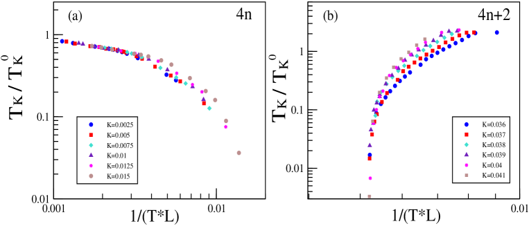
Figure 5: $T_{K}$ as functions of $1/(T^{*}L)$: (a) $L=4n$, $K$ varies from $0.0025t$ to $0.015t$, distance: $0.0025t$. (b) $L=4n+2$, $K$ varies from $0.036t$ to $0.04t$, distance: 0.001t. $T_{K}$ follows universal scaling functions of $1/(T^{*}L)$. Other parameters: $\epsilon_{d}$ = -0.8t, $t_{R}$ = $t_{L}$ = 0.4t, $\phi=0$. Here, we set $t=1$.

.3.5 C. Local Density of State

We now turn our attention to the local density of states (LDOS) on the dot $1$, given by

$$\rho_{QD}(\omega) =-\frac{1}{\pi}Im{G^{R}}_{d_{1}d_{1}}(\omega)$$ (14)

where $G^{R}_{d_{1}d_{1}}(t)\equiv<d_{1}(t)d_{1}^{\dagger}(0)>$ is the retarded Green’s function of dot $1$ which directly couples to the ring. Near the Fermi surface, $\rho_{QD}(\omega)$ determines the transport properties of the system, and it can be obtained from the Green’s function ${G}_{d_{1}d_{1}}(\omega)$ via equation of motion approach. First, the mean-field Hamiltonian in momentum space is given by:

$$H_{MF} = \sum_{m,\sigma}\epsilon_{m}c_{m}^{\dagger}c_{m}+H.C.+\widetilde{\epsilon_{d}}f_{1\sigma}^{\dagger}f_{1\sigma}-\sum_{m}(t_{m}c_{m}^{\dagger}f_{1}+H.C.)$$

$$- \chi f_{1}^{\dagger}f_{2}-H.C.+\frac{\chi^{2}}{K}+\lambda(b_{0}^{2}-1)$$

Where

$$t_{m}={\it i}\sqrt{\frac{2}{L}}\sin({\frac{m}{L}\pi})[\widetilde{t_{L}}+\widetilde{t_{R}}\exp(i\phi)(-1)^{m+1}]$$ (16)

with $m=1,2,\cdots L-1$ring2 .

The equation for a general retarded Green’s function $G_{ij}^{R}(\omega)$ is then given by:

$$(\omega+{\it i}\eta-H_{MF})G_{ij}^{R}(\omega)={\it I}$$ (17)

where ${\it I}$ is the identity matrix, $i,j$ can be $f_{1}$, $f_{2}$, or $m$. We therefore get the following three equations for $G_{f_{1}f_{1}}$, $G_{f_{1}m}$ and $G_{f_{1}f_{2}}$:

$$(\omega+{\it i}\eta-\widetilde{\epsilon_{d}})G_{f_{1}f_{1}}^{R}(\omega)-\chi G_{f_{2}f_{1}}^{R}-\sum_{m}t_{m}G^{R}_{md1}(\omega)=1$$ (18)

$$-\chi G^{R}_{f_{1}f_{1}}+(\omega+{\it i}\eta)G^{R}_{f_{2}f_{1}}=0$$ (19)

$$-t_{m}G^{R}_{f_{1}f_{1}}+(\omega+{\it i}\eta-\epsilon_{m})G^{R}_{mf_{1}}=0$$ (20)

The above equations are easily solved and we get:

$${G}^{R}_{d_{1}d_{1}}(\omega) =b_{0}^{2}G^{R}_{f_{1}f_{1}}=\frac{b_{0}^{2}}{\omega-\widetilde{\epsilon_{d}}+{\it i}\eta\hskip 2.84544pt-\sum_{m}[\frac{t_{m}^{2}{\mid b_{0}\mid}^{2}}{\omega-\epsilon_{m}+{\it i}\eta}]-\frac{\chi^{2}}{\omega+{\it i}\eta}}$$ (21)

where $\eta\rightarrow 0$. We then obtain $\rho_{QD}(\omega)$ by Eq. 14. In the following we analysize the crossover behaviors in LDOS $\rho_{QD}(\omega)$.

.3.6 1. $K=0$

Figure 6: Local density of state for $K=0$ system (in arbitrary unit) (a) $L=4n$ (b) $L=4n+1$ (c) $L=4n+2$ (d) $L=4n+3$. Here, $r=\xi_{k}^{0}/L$, the ratio between $\xi_{k}^{0}$ and $L$. Other parameters: $\epsilon_{d}$ = -0.8t, $t_{R}$ = $t_{L}$ = 0.4t, $\phi=0$. Here, we set $t=1$.

In the absence of the antiferromagnetic spin-spin coupling ($K=0$) the LDOS has been extensively studied where $\rho_{QD}(\omega)$ depends sensitively on $L$ (mod$4$) at finite sizes ring2 . As shown in Fig.(6), our results on LDOS in this case at finite sizes are qualitatively in good agreement with that in Ref.ring2 . For the convenience of later discussions we summarize below the behaviors of LDOS in the four different cases of $L$. The key features are– (i). There exsits a main Kondo resonance peak (located either symmetrically or asymmetrically with respect to $\omega=0$) followed by pairs of side peaks. (ii). As shown in Fig. 6, as $L$ increases the main Kondo peak gets more pronounced and closer to $\omega=0$; while the side peaks are gradually merged into the broadened main peak. In particular, the LDOS for $L=4n$ is very symmetric $\rho_{QD}(\omega)=\rho_{QD}(-\omega)$, suggesting the symmetry between particle and hole excitation energy in the finite size spectrum. The asymmetric Kondo peaks for $L=4n+1$ and $L=4n+3$ are located on the opposite sides (left for $L=4n+1$ and right for $L=4n+3$) of $\omega$. For $L=4n+2$, however, the LDOS shows asymmetric double Kondo peaks with comparable sizes and a dip at $\omega=0$. These differences in DOS among the four sizes of $L$ (mod $4$) can be explained in terms of the energy levels corresponding to the highest occupied (HO) and the lowest unoccupied (LU) states relative to the Fermi levelring2 : For $L=4n$, both HO and LU levels are around the Fermi energy $\epsilon_{F}=0$, leading to a symmetric single peak in LDOS at $\omega=0$. For $L=4n\pm 1$, HO and LU levels are both below and above $\epsilon_{F}$, respectively, giving rise to an asymmetric single peak in LDOS below and above $\omega=0$ separately. However, for $L=4n+2$, LO and HU levels are on the opposite side of the Fermi level, resulting in splitted double Kondo peaks below and above $\omega=0$. It should be noted that despite the differences at finite sizes ($L\sim\xi_{k}^{0}$), the LDOS in all four cases indeed merges to a single Kondo peak as the system reaches the thermodynamic limit $L\rightarrow\infty$ (or $L\gg\xi_{k}^{0}$). (iii). The LDOS on dot $1$ obeys the following symmetriesring2 : $\rho_{QD}^{L}(\omega,\phi)=\rho_{QD}^{L+2}(\omega,\phi+\pi)$ and $\rho_{QD}(-\omega,\phi)=\rho_{QD}(\omega,\phi+\pi)$.

We would like to point out here that from the width $D$ of the central Kondo peak(s), which can be approximately regarded as a quantity proportional to the effective Kondo temperature $T_{k}$, in LDOS for $K=0$ case one can qualitatively understand the opposite trends in $T_{k}$ at finite sizes in case (I) and (II) mentioned above. For $L=4n,4n+1,4n+3$ (case (I)), the width $D$ becomes larger as $L$ increases, indicating an increase in $T_{k}$ as the system approaches to the thermodynamic limit; while as for $L=4n+2$ (case (II)), $D$ gets smaller as $L$ increases, suggesting a decrease in $T_{k}$ as $L\rightarrow\infty$. We analysize in details below the behaviors of LDOS for $K>0$.

.3.7 2. $K>0$

At a finite $K>0$, the LDOS on the dot shows a crossover between the Kondo phase and the spin-singlet phase. For $K<K_{c1}$ at a fixed size $L$, the LDOS remains the same as that for $K=0$. For $L=4n,4n+2$ we find a continuous evolution in LDOS from Kondo to the crossover region near $K=K_{c1}$; while for $L=4n+1,4n+3$ the LDOS exhibits a first-order jump at $K_{c1}$. For $K>K_{c2}$, we find $\rho_{QD}(\omega)=0$ as the indicator of the local spin-singlet phase since $b_{0}=0$. In the crossover region $K_{c1}<K<K_{c2}$, the Kondo peak in LDOS splits into two with respective to $\omega=0$. The splitting gets wider as $K$ increases further. Details are shown below.

.3.8 (i). Varies $K$ with fixed $L$:

Figure 7: Local density of state (in arbitrary unit) with various $K$ for $r=\xi_{k}^{0}/L\sim 0.53$. (a) $L=4n$ (b) $L=4n+1$ (c) $L=4n+2$ (d) $L=4n+3$. Other parameters: $\epsilon_{d}$ = -0.8t, $t_{R}$ = $t_{L}$ = 0.4t, $\phi=0$. Here, $K$ is in unit of $t$, and we set $t=1$.

In Fig.7, we show LDOS for various antiferromagnetic spin-spin coupling strength $K$ at a fixed size $L\approx 200$ ($\xi_{k}^{0}/L\sim 0.5$). The behaviors of LDOS are classified by $L$(mod $4$). The common features in Fig. 7 are as follows. In each of the four LDOS plots in Fig. 7, the Kondo peak in $\rho_{QD}(\omega)$ splits into two at a small value of $K>K_{c1}$, indicating the crossover between Kondo and local spin singlet phases. The two peaks separate further apart and become more symmetric as $K$ increases. At the end, $\rho_{QD}(\omega)$ vanishes when $K>K_{c2}$ in the local spin singlet phase. Note that the values for $K_{c2}$ depend sensitively on $L$ (mod $4$). This can be understood as when $L\approx 200$ the effective Kondo temperature $T_{k}$ in case (II) is much larger than that in case (I) (see Fig.4, Fig. 5) , which explains why we need a larger value of $K_{c2}$ in case (II) to suppress the Kondo effect than that in case (I). We present details below.

.3.9 (ii). Varies $L$ with fixed $K$:

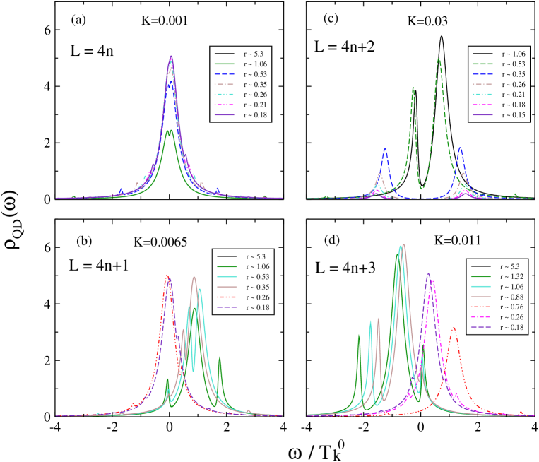
Figure 8: Local density of state (in arbitrary unit) with various $L$ and fixed $K$ (in unit of $t$). Here, $r=\xi_{k}^{0}/L$. (a) $L=4n$ (b) $L=4n+1$ (c) $L=4n+2$ (d) $L=4n+3$. Other parameters: $\epsilon_{d}$ = -0.8t, $t_{R}$ = $t_{L}$ = 0.4t, $\phi=0$. Here, we set $t=1$.

Fig. (8) shows how $\rho_{QD}(\omega)$ changes with the system size $L$. For $0<K<K_{c}$, starting from a small size $L<L_{c1}$, the LDOS changes from the behavior of a local spin-singlet state with $\rho_{QD}(\omega)=0$ to that in the crossover region with splitted peaks and finite LDOS at $\omega=0$, and finally it recovers the Kondo resonance at larger size $L>L_{c2}$.

We separate the discussion here into two different cases: $K<K_{c}$ (case (I)) and $K>K_{c}$ (case (II)). Fig.(8(a),(b),(d))show finite size dependence of $\rho_{QD}(\omega)$ at $K<K_{c}$ (case (I)) for $L=4n$, $4n+1$, and $4n+3$, respectively. For small system sizes, the system is in the local spin-singlet state with vanishing LDOS. At intermediate sizes in the crossover region, however, LDOS starts to develop peaks with a dip at $\omega=0$. As size further increases, these splitted peaks either gradually ($L=4n$) or suddenly ($L=4n+1$ and $4n+3$) merge into a single Kondo peak located either symmetrically ($L=4n$) or asymmetrically ($L=4n+1$ and $4n+3$) with respect to $\omega=0$. These Kondo peaks then follow the evolution at finite sizes for $K=0$ and finally recover the single symmetric Kondo peak in the thermodynamic limit.

For $K>K_{c}$ (case (II)), the size dependence of $\rho_{QD}(\omega)$ is shown in Fig.(8(c)) with $K=0.03t>K_{c}$. The LDOS exhibits a crossover from the Kondo to local spin-singlet state with increasing size $L$. For $K\sim K_{c}$ the LDOS changes from singlet state at small sizes to the crossover regime within the range $100<L<800$ that we investigate. To study the the ultimate fate of the system one needs to go much larger system size than $L\sim 800$, which is beyond the scope of our computational limit. Note that our analysis on the LDOS by changing $K$ with fixed $L$ (changing $L$ with fixed $K$) is consistent with the green line (red line) of the schematic phase diagram shown in Fig. (2). Finally, the first order jumps seen in LDOS at $K=K_{c1}$ for $L=4n+1$ and $L=4n+3$ may be due to the artifact of the mean-field theory. Further investigation is needed to clarify this issue.

.3.10 D. Persistent Current

We now analysize the crossover from the behaviors in persistent current. The Kondo screening cloud in our closed setup is restricted itself in the ring. To get an experimental access, one possible way is to measure persistent current (PC) induced by changing the magnetic flux threading the ring without attaching leads to it. PC is defined as:

$$I=-\frac{e}{\hbar}\frac{\partial E_{gs}}{\partial\phi}$$ (22)

PC can be served as a detector for the Kondo screening cloud since as a function of $\phi$ PC behaves very differently when $\xi_{k}\gg L$ than when $\xi_{k}\ll L$. Such persistent current experiments have been reported recently on micron sized ring without containing the dotPCexp . In our setup, PC can be used to measure the strength of the Kondo correlation as the antiferromagnetic coupling $K$ is expected to suppress the Kondo effect, leading to a weaker PC.

.4 K=0

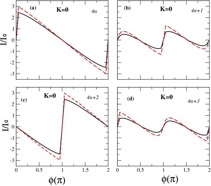
Figure 9: Persistent current (in unit of $I_{0}$) versus magnetic flux (in unit of $2\pi/\Phi_{0}$) with $K=0$. Red dashed line is for $r=\xi_{k}^{0}\sim 0.53$. Black solid line is for $\xi_{k}^{0}/L\sim 1.06$. (a) $L=4n$ (b) $L=4n+1$ (c) $L=4n+2$ (d) $L=4n+3$. Other parameters: $\epsilon_{d}$ = -0.8t, $t_{R}$ = $t_{L}$ = 0.4t. Here, we set $t=1$.

Before we present our new results on the PC, it proves useful to summarize the previous resultsring1 ring2 for $K=0$. As shown in Fig.(9), since the system is in the Kondo regime, PC increases with increasing system size $L$. PC as a function of the magnetic flux is a weak sinusoidal wave when $L\ll\xi_{k}^{0}$; while it behaves like a saw-tooth when $L\gg\xi_{k}^{0}$. Meanwhile, there exists a relation between PC for $L$ and $L+2$: $I_{N}(\phi)=I_{N+2}(\phi+\pi)$ring1 ring2 due to the $\pi$ shift in LDOS of the quantum dot from the system with $N$ sites to $N+2$ sites. Furthermore, the magnitude of PC for $L=odd$ is much smaller than that for $L=even$. This can be understood as for $L=odd$ the electrons are fully occupied at the Fermi level, which suppresses the Kondo resonance; while as for $L=even$ there is an unpaired electron on the Fermi level, leading to the Kondo resonance. The results for $K>0$ are shown below.

.4.1 1. Varies $K$ with fixed $L$:

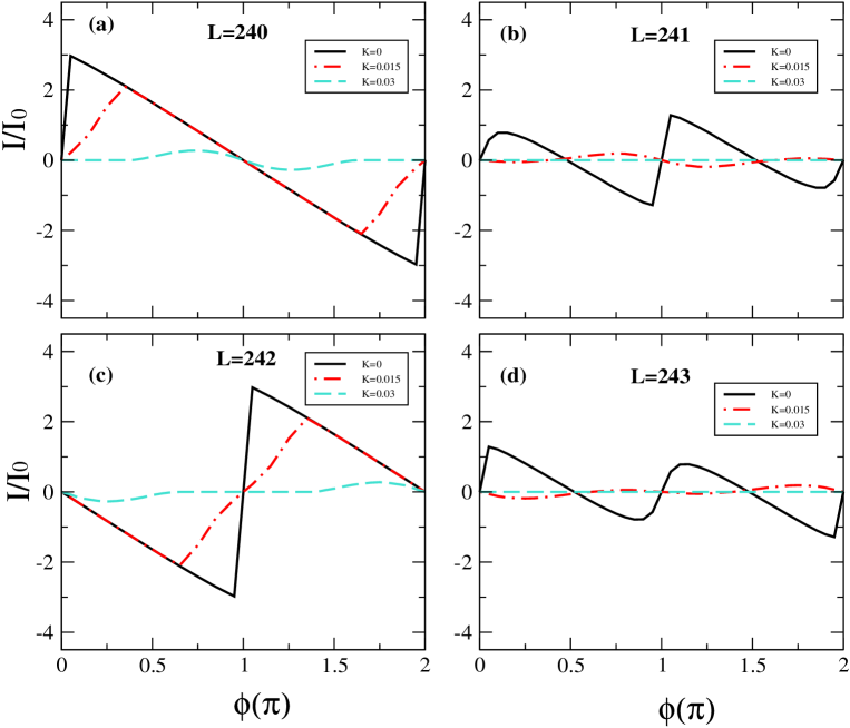
Figure 10: PC versus $\phi$ with various $K$ for $L\sim 240$ ($\xi_{k}^{0}/L\sim 0.44$). $K=0,0.015,0.03$ (in unit of $t$) (a) $L=4n$ (b) $L=4n+1$ (c) $L=4n+2$ (d) $L=4n+3$. Other parameters of data: $\epsilon_{d}$ = -0.8t, $t_{R}$ = $t_{L}$ = 0.4t. Here, we set $t=1$.

PC (in unit of $I_{0}$ where $I_{0}=ev_{F}/L$ is the persistent current of an ideal metallic ring with $v_{F}$ being Fermi velocity) versus magnetic flux with different antiferromagnetic coupling strength $K$ at a finite size $L\sim 240$ ($\xi_{k}^{0}/L\sim 0.44$) is shown in Fig.(10). The general trend in all four cases is that the amplitude of PC gets smaller as $K$ is increased and finally vanishes for $K>K_{c2}$, in agreement with the expectation on the suppression of the Kondo effect by the antiferromagnetic spin-spin coupling. Also, as shown in Fig. 10, the shape of the PC as a function of $\phi$ changes from saw-tooth shape at smaller $K$ values to weak sinusoidal waves at larger $K$ values, similar to that for $K=0$. There are detail differences among the four cases. In Fig.(10(a) and (c)), with increasing $K$ the persistent current $I_{L=240}$ near $0.5\pi<\phi<1.5\pi$ decreases more slowly than that for $0\pi<\phi<0.5\pi$ and $1.5\pi<\phi<2\pi$; similarily for $I_{L=242}$ except for the range of $\phi$ is being interchanged. This suggests that the Kondo effect is more robust in $0.5\pi<\phi<1.5\pi$ for $L=4n$ and in $0\pi<\phi<0.5\pi$ and $1.5\pi<\phi<2\pi$ for $L=4n+2$. Note that we find the similar jumps at $K=K_{c1}$ mentioned previously in LDOS to also appear in PC for $L=4n+1$ and $L=4n+3$; while PC is continuous at at $K=K_{c1}$ for the other two cases. Despite the above detail differences, we find two common features in Fig. (10) that remain the same as in the case of $K=0$: (i). $I_{N}(\phi)=I_{N+2}(\phi+\pi)$ and (ii). PC for $L=even$ is larger than that for $L=odd$.

.4.2 2. Varies $L$ with fixed $K$:

Fig.(11) and Fig.(12) show PC versus magnetic flux at different system sizes. In the following the discussion is separated into two cases: (i). $K<K_{c}$ (case (I)) where PC increases with increasing size $L$, and (ii). $K>K_{c}$ (case (II)) where PC decreases to $0$ as $L$ reaches the thermodynamic limit.

(i). $K\leq K_{c}$

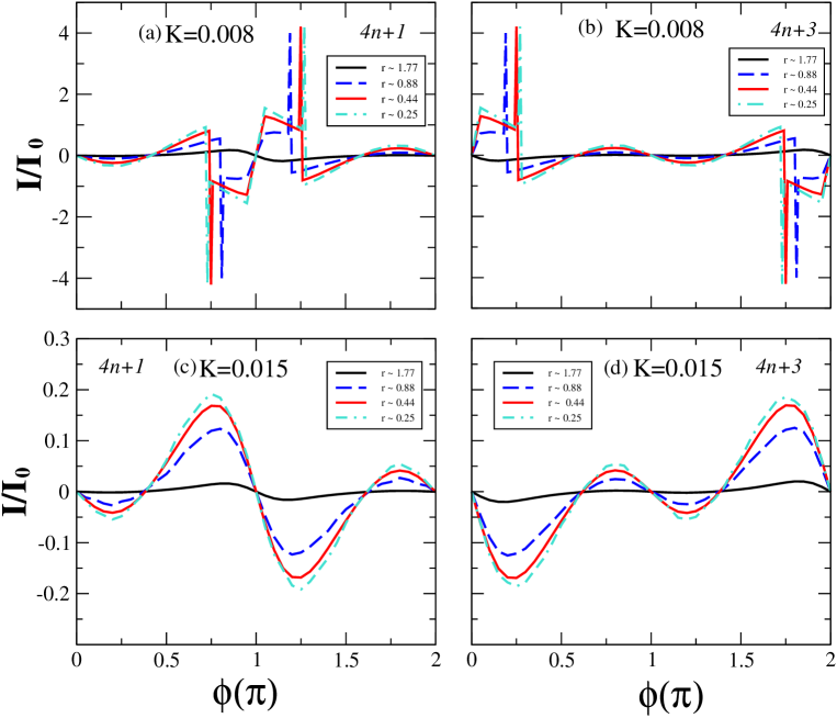
Figure 11: Persistent current with various $L$ and fixed $K$ (in unit of $t$). (a) $L=4n+1$, $K=0.008$ (b) $L=4n+3$, $K=0.008$ (c) $L=4n+1$, $K=0.015$ (d) $L=4n+3$, $K=0.015$. Here, $r=\xi_{k}^{0}/L$. The parameters are: $\epsilon_{d}$ = -0.8t, $t_{R}$ = $t_{L}$ = 0.4t, $\phi=0$. Here, we set $t=1$.

We first look at cases with $K<K_{c}$. Fig.(11) shows PC versus magnetic flux with different size $L$ for $K=0.008$ and $K=0.015$ (in unit of $t$). For $K=0.008$ (see Fig.11(a)(b)), as $L$ is increased we find the PC exhibits two different behaviors: near $\phi=\pi$ for $L=4n+1$ and $\phi=0,2\pi$ for $L=4n+3$ PC changes from the behavior in crossover region to the Kondo state at $K=0$ (see Fig. (9(b)(d)); while out of these ranges of $\phi$ its behavior remains the same as in the crossover region but with an increasing amplitude. A first-order jump is seen to separate these two regions. We expect at much larger system size the Kondo phase will be restored eventually over the entire range of $\phi$. We have also investigated PC for $L=4n,4n+2$ (not shown here) and find the same qualitative behaviors except that instead of jumps we find a continuous change in PC. Also, the behavior in $I_{4n+1}^{\phi\sim\pi}$ (or equivalently $I_{4n+3}^{\phi\sim 0}$) is the same as that for $K=0$ for all the sizes we investigate, suggesting the Kondo phase is very easily restored in these ranges of $\phi$.

On the other hand, for a larger value of $K=0.015$ (see Fig.11(c)(d)), as $L$ increases from $L\sim 60$ to $L\sim 420$ (or $r=\xi_{k}^{0}/L$ changes from $1.77$ to $0.25$) PC still stays in the crossover region with an increasing amplitude. This is expected as for larger value of $K$ one must go to much larger system size to observe the restoring of the Kondo effect in PC.

(ii). $K\geq K_{c}$

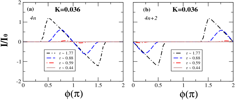
Figure 12: Persistent current with various $L$ and fixed $K$. (a) $L=4n$ (b) $L=4n+2$. Here, $r=\xi_{k}^{0}/L$. Other parameters of data: $\epsilon_{d}$ = -0.8t, $t_{R}$ = $t_{L}=0.4t$, $K=0.036$ (in unit of $t$). Here, we set $t=1$.

We now investigate the case where $K>K_{c}$. As shown in Fig.(12), since $K>K_{c}$ in this case, PC decreases in amplitude with increasing system size $L$ and finally the system reaches the local spin-singlet state with vanishing PC. Note that $I_{4n}^{\phi\sim 0}$ and correspondingly $I_{4n+2}^{\phi\sim\pi}$ are always vanishingly small for all the sizes we investigate, suggesting the systems are already in the local spin-singlet states from the start for these ranges of $\phi$, which is consistent with our mean-field phase diagram. However, for the remaining ranges of $\phi$ the systems start from the crossover region for smaller sizes and reach finally to the local spin-singlet state at large size.

From above results for PC, it implies that by applying magnetic flux, we may change the ground state of our system at finite sizes either from the local spin-singlet state to the crossover region or from the Kondo phase to the crossover region.

.5 IV. Conclusions

To summarize, we have studied via large-N slave-boson mean-field approach the Kondo effect in a side-coupled double-quantum-dot system where one dot is embedded in a mesoscopic ring. The competition between the Kondo effect and the antiferromagnetic spin-spin interaction in this geometry gives rise to the Kosterlitz-Thouless quantum phase transition with a finite critical value $K_{c}$ in the thermodynamic limit. The mean-field phase diagrams of the model depends on the finite size $L$ (mod $4$): for $L=4n,4n+1,4n+3$ (case (I)) the crossover occurs for $K<K_{c}$; while for $L=4n+2$ (case (II)) the crossover exists for $K>K_{c}$. To further study how the Kondo screening is suppressed by the RKKY, we have performed a systematic finite-size analysis on the Kondo temperature $T_{k}$, the local density of states on the dot $\rho_{QD}(\omega)$ which connects to the ring , and the persistent current PC induced by the magnetic flux penetrating through the ring. For a fixed $K<K_{c}$, we find all the above quantities flow to the Kondo phase (same phase as in $K=0$) with increasing system size: $T_{k}$ and PC increase in magnitude and $\rho_{QD}(\omega)$ develops a pronounced single Kondo peak centered at $\omega=0$; while for $K>K_{c}$, the flow at finite sizes is towards to the local spin-singlet phase where all of the three observables decrease in magnitude to $0$ with increasing size. From the finite-size scaling of $T_{k}$, we have shown that $T_{k}$ is an universal function of $1/(LT^{*})$ for $1/L<T^{*}$ where $T^{*}$ has been unambiguously identified the characteristic Kosterlitz-Thouless crossover energy scale: $T^{*}=c\widetilde{T_{k}}\exp{[-\pi\widetilde{T_{k}}/(K-K_{c})]}$. For a fixed size $L$, we find the ground state remains in the Kondo phase for $K<K_{c1}$ and it crossovers to the local spin-singlet phase for $K_{c1}<K<K_{c2}$ and finally reaches the spin-singlet phase for $K>K_{c2}$. For $L=4n+1,4n+3$, we find the first order jumps in all of the three observables at the phase boundary between Kondo and the crossover region. Whether these first order jumps are the artifacts of the large-N mean-field theory is yet to be clarified. Note that unlike the similar system studied previously on the side-coupled double-dot system embedded in conduction electron Fermi sea with constant density of states, the key finding in this paper is the KT transition with a finite critical value $K_{c}>0$ in a side-coupled double-dot system embedded in a mesoscopic ring (in stead of $K_{c}=0$ for the system with Fermi sea of continuous spectrum). Whether this finite $K_{c}$ is due to the artifact of the mean-field theory or due to the more singular density of states of the 1D tight-binding ring needs further investigations. Our results on the transport properties of the system are relevant for future experiments on the side-coupled double-quantum-dot system embedded in a mesoscopic ring.

- (1) A. C. Hewson,The Kondo Problem to Heavy Fermions (Cambridge University Press, Cambridge, England, 1997).
- (2) L. Kouwenhoven and L. Glazman, Phys. World 14, 33 (2001).
- (3) D. Goldharber-Gorden, H. Shtrikman, D. Mahalu, D. Abusch-Magder, U. Meirav, and M.A. Kaster, Nature (London) 391, 156 (1998); S. M. Cronenwett, T.H. Oosterkamp, and L.P. Kouwenhoven, Science 281, 540 (1998); For a review: D. Goldharber-Gorden et al. Material Science and Engineering B 84, 17-21 (2001).
- (4) I. Affleck and P. Simon, Phys. Rev. Lett. 86, 2854 (2001); P. Simon, I. Affleck, Phys. Rev. B 64, 085308 (2001).
- (5) Hui Hu, Guang-Ming Zhang, and Lu Yu, Phys. Rev. Lett. 86, 5558 (2001).
- (6) Kicheon Kang and Sung-Chul Shin, Phys. Rev. Lett. 85, 5619 (2000).
- (7) K. G. Wilson, Rev. Mod. phys. 47, 773 (1975).
- (8) N. J. Craig, J. M. Taylor, E. A. Lester, C. M. Marcus, M. P. Hanson, A. C. Gorssard, Science 304, 565 (2004).
- (9) Gergely Zerand, Chung-Hou Chung, , Phys. Rev. Lett. 97, 166802 (2006).
- (10) Pascal Simon, Rosa Lopez, and Yuval Oreg, phys. Rev. Lett. 94, 086602 (2005).
- (11) P. S. Cornaglia and D. R. Grempel, Phys. Rev. B 71, 075305 (2005)
- (12) Pascal Simon, Phys. Rev. B 71, 155319 (2005).
- (13) B.A. Jones, C.M. Varma, and J.W. Wilkins, Phys. Rev. Lett. 61, 125 (1988); B.A. Jones, C.M. Varma Phys. Rev. B 40, 324 (1989); I. Affleck, A.W. Ludwig and B.A. Jones, Phys. Rev. B 52, 9528 (1995).
- (14) C. H. Chung, G. Zarand, and P. Woelfle, Phys. Rev. B 77, 035120 (2008)
- (15) Luis G. G. V. Dias da Silva, Nancy Sandler, Pascal Simon, Kevin Ingersent, and Sergio E. Ulloa, Phys. Rev. Lett. 102, 166806 (2009).
- (16) M. Buttiker and C.A. Stafford, Phys. Rev. Lett. 76, 495, (1996); Pascal Cedraschi, Vadim V. Ponomarenko, and Markus Büttiker, Phys. Rev. Lett. 84, 346 (2000).
- (17) J. Brad Marston and Ian Affleck, Phys. Rev. B 39, 11538 (1989).
- (18) V. Chandrasekhar, R.A. Webb, M.J. Brady, M.B. Ketchen, W.J. Gallagher and A. Kleinsasser, Phys. Rev. Lett. 67, 3578 (1991); D. Mailly, C. Chapelier and A. Benoit and B. Etienne, cond-mat/0007396.