UT-09-17

IPMU09-0088

TU-850

Non-thermal Gravitino Dark Matter in Gauge Mediation

Koichi Hamaguchi^1,2, Ryuichiro Kitano³, Fuminobu Takahashi²

¹ Department of Physics, University of Tokyo, Tokyo 113-0033, Japan
² Institute for the Physics and Mathematics of the Universe, University of Tokyo,
Chiba 277-8568, Japan
³ Department of Physics, Tohoku University, Sendai 980-8578, Japan

1 Introduction

The presence of dark matter (DM) in the Universe was firmly established by numerous observations [1]. Nevertheless, it has remained as a big mystery in cosmology as well as particle physics what DM is made of. Since there is no candidate for DM in the standard model, we need to consider new physics.

In a supersymmetric extension of the standard model, the lightest supersymmetric particle (LSP) is a stable particle if the $R$ parity is conserved. Depending on the mediation mechanism of the supersymmetry (SUSY) breaking effects, the lightest neutralino or the gravitino can thus be a good candidate for DM. The latter possibility is naturally realized in a framework of gauge mediation [2, 3], which has a virtue of avoiding the SUSY flavor problem.

The production mechanisms of gravitinos in the early Universe are broadly classified into thermal or non-thermal one. The thermal production is always present as long as the Universe becomes radiation dominated after inflation [4, 5, 6, 7, 8, 9, 10]. In this case the decay rate of an inflaton must be such that gravitinos, produced by particle scatterings in thermal plasma, account for the observed DM abundance. If the inflationary dynamics has nothing to do with the SUSY breaking mechanism (and therefore the gravitino mass), such a coincidence may call for some explanation. On the other hand, non-thermal gravitino production has been discussed (mostly as a problem of overproduction or a solution to it) in the context of the decay of the next to lightest SUSY particle (NLSP) [11, 12], the moduli [13, 14, 15, 16, 17, 18], the inflaton [19, 20, 21, 22, 23, 24, 25, 26] and the SUSY breaking field (sometimes called as the Polonyi field or the pseudo-moduli field) [27, 28, 29, 30, 31, 32, 34]. In particular, it is interesting to see if a right amount of the gravitinos can be produced by the decay of the SUSY breaking field, since the structure of the SUSY breaking sector may be probed by cosmological arguments.

In this paper, we investigate the gravitino DM scenario in a generic setup of gauge-mediated SUSY breaking models. In many SUSY breaking models, there is a light singlet scalar field, which obtains a mass from SUSY breaking. During the inflation era, this scalar field, the pseudo-moduli field, can have a large displacement from the true vacuum, and at a later time, it starts coherent oscillations about the minimum of the potential. Under reasonable assumptions, the oscillation energy dominates the energy density of the Universe, and the decay of the scalar field produces radiation as well as gravitinos which remain as DM today. We update the calculation of Ref. [32] by taking into account the following points. We do not assume a particular relation among parameters in the SUSY breaking sector. We treat the real and the imaginary parts of the scalar field separately as their decay properties are quite different. We find that, for the mass of the scalar field around ${\cal O}(100)$ GeV and the gravitino mass of ${\cal O}(10-100)$ MeV, the decay of the imaginary part is the main source of the radiation and the gravitinos that account for the observed DM abundance. The region turns out to be similar to the one found in Ref. [32] although the main decay mode is different. The consistent region overlaps with the prediction of a model in Ref. [33] where the $\mu$ problem is solved.

2 Gauge mediation

We first define the framework and identify parameters relevant for the discussion of cosmology. We use an effective description of gauge-mediation models given in terms of a SUSY breaking field $S$ and the fields in the minimal SUSY standard model (MSSM). The SUSY breaking sector is described by a single chiral superfield $S$ which consists of the Goldstino fermion and its scalar partner $s$ with the Kähler and super-potentials:

$$K=S^{\dagger}S-{(S^{\dagger}S)^{2}\over\Lambda^{2}}+({\mbox{higher order}}),$$ (1)

$$W=m^{2}S,$$ (2)

where $\Lambda$ is a cut-off scale of the effective theory, and $m$ denotes the size of the SUSY breaking. This form is obtained after integrating out massive fields in a wide class of SUSY breaking models. The equation of motion gives $F_{S}=m^{2}$ as long as there is no singularity in the Kähler potential. The second term in Eq. (1) stabilizes the scalar potential at $s=0$.

The MSSM particles can couple to the SUSY breaking sector through messenger fields, $f$ and $\bar{f}$:

$$W\ni-\lambda Sf\bar{f},$$ (3)

where $\lambda$ is a dimensionless coupling constant. With this term, the potential is minimized at $s=0$ and $f\bar{f}=m^{2}/\lambda$ where SUSY is unbroken and the gauge symmetry of the MSSM is broken. Therefore, one needs some mechanism to stabilize the potential at $\langle s\rangle\neq 0$ and $\langle f\rangle=\langle\bar{f}\rangle=0$.

In order to keep discussion as general as possible, we do not specify such a mechanism in the following and treat the three quantities ($\langle s\rangle$, $F_{S}$, $\Lambda$) as independent parameters. Here we define the origin of the $s$ field to be the point where the messenger fields become massless, i.e., $M_{\rm mess}=\lambda\langle s\rangle$. Once we integrate out the messenger fields, the gauge kinetic term in this case is given by

$$f={1\over 2}\left({1\over g^{2}}-{2N\over(4\pi)^{2}}\log{S\over\Lambda}\right)W^{\alpha}W_{\alpha}+{\rm h.c},$$ (4)

where $g$ is the gauge coupling constant and $N$ is the (effective) number of messenger fields. Our later discussion can apply when the low energy effective theory is of this type. For example, in the model of Ref. [35] the supergravity effects create a local minimum at $\langle s\rangle\sim\Lambda^{2}/M_{\rm Pl}$, where $M_{\rm Pl}\simeq 2.4\times 10^{18}$ GeV is the reduced Planck scale. Ref. [36] discussed a model with an additional superpotential term, $W\ni M_{\rm mess}f\bar{f}$, with which the effective value of $\langle s\rangle$ is $M_{\rm mess}/\lambda$.

The important point here is that the scalar field $s$ couples to the MSSM fields with a suppression of $F_{S}/\langle s\rangle^{2}$, whereas the coupling to the gravitino is suppressed by $F_{S}/\Lambda^{2}$. Therefore, for $\langle s\rangle\ll\Lambda$, there is a possibility to avoid the dangerous gravitino overproduction as well as the catastrophic entropy release from the $s$ decay [37, 27, 29, 30, 15, 16, 17, 31].

The three parameters $\langle s\rangle$, $F_{S}$, and $\Lambda$ can be expressed in terms of physical quantities relevant for our discussion, such as the masses of Bino, $s$, and gravitino [$m_{\tilde{B}}$, $m_{S}$, $m_{3/2}$]. They are related to $\langle s\rangle$, $F_{S}$, and $\Lambda$ as

$$m_{\tilde{B}} = {g_{1}^{2}N\over(4\pi)^{2}}{F_{S}\over\langle s\rangle},$$ (5)

$$m_{S} = {2F_{S}\over\Lambda},$$ (6)

$$m_{3/2} = {F_{S}\over\sqrt{3}M_{\rm Pl}},$$ (7)

where $g_{1}=\sqrt{5/3}g_{Y}$ with $g_{Y}$ being the coupling constant of the U(1)_Y gauge interaction. When expressed in terms of the running Bino mass at the electroweak scale, explicit $\lambda$ dependence of the low energy quantities disappears in many places. We can invert the above relations and write $\langle s\rangle$, $F_{S}$, and $\Lambda$ in terms of the physical quantities:

$$F_{S} = 1.3\times 10^{17}{\rm\,GeV}^{2}\left(\frac{m_{3/2}}{30~{}{\rm MeV}}\right),$$ (8)

$$\langle s\rangle = 8.6\times 10^{11}{\rm\,GeV}\cdot N\,\left(\frac{m_{3/2}}{30~{}{\rm MeV}}\right)\left(\frac{m_{\tilde{B}}}{200~{}{\rm GeV}}\right)^{-1},$$ (9)

$$\Lambda = 2.5\times 10^{15}{\rm\,GeV}\left(\frac{m_{3/2}}{30~{}{\rm MeV}}\right)\left(\frac{m_{S}}{100~{}{\rm GeV}}\right)^{-1}.$$ (10)

Here and in what follows, we use $m_{3/2}=30~{}{\rm MeV}$, $m_{\tilde{B}}=200~{}{\rm GeV}$ and $m_{S}=100~{}{\rm GeV}$ as reference values, though the following discussion is generic and does not depend on those explicit values.

Although $\lambda$ does not appear in the above relations, it cannot take an arbitrary value. In fact, there are lower and upper bounds on $\lambda$ to avoid instabilities at the SUSY breaking minimum. In order to avoid a tachyonic mass for the messenger fields, $\lambda$ should satisfy $\lambda^{2}\langle s\rangle^{2}>\lambda F_{S}$, i.e.,

$$\lambda>\lambda_{\rm min}=1.7\times 10^{-7}\cdot N^{-2}\left(\frac{m_{3/2}}{30~{}{\rm MeV}}\right)^{-1}\left(\frac{m_{\tilde{B}}}{200~{}{\rm GeV}}\right)^{2}.$$ (11)

On the other hand, the interaction term in Eq. (3) induces a logarithmic potential at one-loop level [32, 35],

$$V(s)=m_{S}^{2}|s-\langle s\rangle|^{2}+\frac{5N}{16\pi^{2}}\lambda^{2}F_{S}^{2}\log\left(\frac{|s|^{2}}{\Lambda^{2}}\right),$$ (12)

where we have assumed that the messenger fields transform as ${\bf 5}$ and $\bf{\bar{5}}$ under SU(5). The logarithmic potential gives an attractive force on the $s$ field toward the SUSY vacuum at the origin. The stability at the SUSY breaking minimum requires

$$\frac{5N}{16\pi^{2}}\lambda^{2}F_{S}^{2}<\frac{1}{4}m_{S}^{2}\langle s\rangle^{2},$$ (13)

namely

$$\lambda<\lambda_{\rm max}=1.9\times 10^{-3}\cdot N^{1/2}\left(\frac{m_{S}}{100~{}{\rm GeV}}\right)\left(\frac{m_{\tilde{B}}}{200~{}{\rm GeV}}\right)^{-1}.$$ (14)

In the following, we assume $\lambda_{\rm min}<\lambda<\lambda_{\rm max}$. The above logarithmic potential also induces a mass splitting between the real and imaginary parts of the $s$ field, $\delta m^{2}/m_{S}^{2}={\cal O}(\lambda^{2}/\lambda_{\rm max}^{2})$, as well as a shift of the minimum, $\delta\langle s\rangle/\langle s\rangle={\cal O}(\lambda^{2}/\lambda_{\rm max}^{2})$. For simplicity, we assume $\lambda^{2}\ll\lambda_{\rm max}^{2}$ and neglect those corrections in the following discussion.

3 Scenario

Let us first give an overview of the cosmological scenario in this model; (i) the $s$ field develops a large expectation value during the inflation, (ii) its coherent oscillations after the inflation dominate the energy density of the Universe, and (iii) its decay produces radiation (including SUSY particles if kinematically allowed) and gravitinos. The assumption (i) is quite natural as far as $m_{S}$ is much smaller than the Hubble parameter $H$ during the inflation, since the minimum of the potential during and after the inflation can be well separated from $s=0$ due to the deformation of the potential through gravitational (or general $1/M_{\rm Pl}$ suppressed) interactions. The $s$ field then starts to oscillate around the minimum when the Hubble parameter becomes comparable to $m_{S}$ and keeps oscillating until it decays.

In the rest of this section, we discuss several conditions for the above scenario to work. An important point here is that there is a global SUSY minimum of the potential at $s=0$, apart from the local SUSY breaking minimum, $s=\langle s\rangle$. Hereafter, we take the basis where $\langle s\rangle$ is real. (See Fig. 1.) As discussed in Ref. [32], the $s$ field does not fall into the SUSY vacuum unless its initial value $s_{\rm ini}$ is too close to the real axis. We investigate in more detail the conditions for $s$ to be trapped at the SUSY breaking minimum. When discussing the dynamics of the $s$ field, we neglect the corrections from higher order terms in the Kähler potential in Eq. (1), which is small as far as $|s|\lesssim\Lambda$.

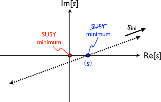
Figure 1: A schematic figure of the evolution of $s$ field.

3.1 Avoiding the SUSY vacuum

If the value of $s$ approaches too close to $s=0$ during the oscillations, the scalar components of the messenger fields may become tachyonic, which makes the Universe quickly fall into the SUSY vacuum. This can be avoided if the initial value for ${\rm Im}[s]$ is so large that the trajectory of $s$ stays away from $s=0$, satisfying

$$|s|>\sqrt{F_{S}\over\lambda}$$ (15)

in the course of oscillations.

Even if the above condition is met, the motion of $s$ can be significantly affected by the deformation of the potential near the origin due to the logarithmic potential Eq. (12). Moreover, it is known that a scalar field oscillating on a scalar potential of the logarithmic form experiences strong spatial instabilities and quickly deforms into spatially random and inhomogeneous state [38]. If such instabilities becomes significant before the $s$ field gets trapped in the SUSY breaking minimum, we expect that it falls into the SUSY vacuum. This can be avoided if the logarithmic correction remains subdominant along the trajectory passing near the origin, i.e., $|s|\ll\left\langle s\right\rangle$, and the condition is given by

$$|s|^{2}\;\gtrsim\;\frac{5N}{16\pi^{2}}\frac{\lambda^{2}F_{S}^{2}}{m_{S}^{2}}.$$ (16)

More rigorous derivation of (16) can be found in Appendix A.

The minimum value of $|s|$ during the oscillations is approximately given by (cf. Fig. 1)

$$|s|_{\rm min} \simeq \langle s\rangle\frac{{\rm Im}[s_{\rm ini}]}{|s_{\rm ini}|}\,,$$ (17)

where $s_{\rm ini}$ is the value of $s$ when it starts coherent oscillations at $H\sim m_{S}$. We can rewrite the constraints (15) and (16) respectively in terms of the ratio of the initial amplitudes, $r\equiv\left|{{\rm Im}[s_{\rm ini}]/{\rm Re}[s_{\rm ini}]}\right|$, as

$$\frac{r}{\sqrt{1+r^{2}}} \gtrsim 0.013\cdot N^{-1}\left(\lambda\over 10^{-3}\right)^{-1/2}\left(m_{\tilde{B}}\over 200~{}{\rm GeV}\right)\left(\frac{m_{3/2}}{30~{}{\rm MeV}}\right)^{-1/2},$$ (18)

$$\frac{r}{\sqrt{1+r^{2}}} \gtrsim 0.26\cdot N^{-1/2}\left(\frac{\lambda}{10^{-3}}\right)\left(\frac{m_{\tilde{B}}}{200~{}{\rm GeV}}\right)\left(\frac{m_{S}}{100{\rm\,GeV}}\right)^{-1}.$$ (19)

In order to study the spatial instabilities, we separate the $s$ field into a homogeneous part ${\bar{s}}$ and a perturbation $\delta s$. We have numerically followed the evolution of ${\bar{s}}$ and $\delta s$ for a set of reference values of $m_{3/2}$, $m_{\tilde{B}}$, $m_{S}$, and $N$, keeping only terms linear in $\delta s$. The initial conditions are set as ${\rm Re}[s_{\rm ini}]=\sqrt{2}\Lambda\cos\theta$ and ${\rm Im}[s_{\rm ini}]=\sqrt{2}\,\Lambda\sin\theta$, where $\theta$ is related to $r$ as $\tan\theta=r$. We have chosen the initial value of $|\delta s|$ equal to $10^{-5}\Lambda$, but the following result is not sensitive to this value. (Indeed, we have confirmed that the result remains almost intact for $|\delta s|=10^{-10}\Lambda$.) In Fig. 2 we show a parameter region surrounded by a solid (green) where $\delta s$ remains smaller than ${\bar{s}}$ until the $s$ field settles down in the SUSY breaking minimum. The allowed regions are found to be $10^{-7}\lesssim\lambda\lesssim 10^{-3}$ and $0.03\lesssim\theta\leq\pi/2$. For different values of $m_{3/2}$, $m_{\tilde{B}}$ and $m_{S}$, the allowed regions are modified correspondingly; in particular, the minimum value of $\theta$ can be smaller. Note that $\delta s\sim{\bar{s}}$ does not necessarily mean that the $s$ field falls into the supersymmetric vacuum. What we would like to emphasize here is that there is a parameter space where our scenario is realized. We have also shown in the figure the conditions (18) and (19), and the latter gives a slightly milder constraint on $\lambda$ than the solid (green) line.

Another concern is whether the ratio of the energy densities of ${\rm Im}[s]$ and ${\rm Re}[s]$, $r_{\rm eff}^{2}\equiv\rho_{s_{I}}/\rho_{s_{R}}$, is conserved or not. According to our numerical calculations, the final value of $r_{\rm eff}$ is always larger or equal to $r$, and $r_{\rm eff}$ tends to become larger for smaller $\theta$ and larger $\lambda$. For most of the region surrounded by the solid (green) line, however, the ratio does not significantly evolve, and in particular, it remains almost constant in the course of evolution for $\theta>0.1$ and $\lambda<10^{-4}$. Therefore we do not distinguish $r_{\rm eff}$ from $r$ in the following discussion. In the above analysis we have not taken into consideration thermal effects, which will be discussed in Appendix B.2.

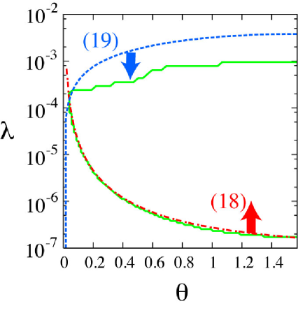
Figure 2: The region surrounded by the solid (green) line represents a parameter space where the perturbation $\delta s$ remains smaller than the homogeneous part ${\bar{s}}$ until the $s$ field gets stabilized at the SUSY breaking minimum. The conditions (18) and (19) are also shown as the dot-dashed (red) and dashed (blue) lines. We have chosen $m_{3/2}=30~{}{\rm MeV}$, $m_{\tilde{B}}=200~{}{\rm GeV}$, $m_{S}=100~{}{\rm GeV}$, and $N=1$.

3.2 $s$-dominated Universe

We assume that the initial value of $|s|$ is so large that the coherent oscillations of $s$ dominate over the energy density of the Universe before the time it decays. Such a domination happens if

$$T_{d}^{(R)} < {\rm min}(T_{R},T_{m_{S}})\left(|{\rm Re}[s_{\rm ini}]-\langle s\rangle|\over\sqrt{3}M_{\rm Pl}\right)^{2}$$ (20)

$${\rm or}~{}~{}~{}$$

$$T_{d}^{(I)} < {\rm min}(T_{R},T_{m_{S}})\left(|{\rm Im}[s_{\rm ini}]|\over\sqrt{3}M_{\rm Pl}\right)^{2}$$ (21)

where $T_{d}^{(R/I)}$ are the decay temperatures of $s_{R/I}$ (cf. next section), $T_{R}$ is the reheating temperature after the inflaton, and $T_{m_{S}}$ is the temperature at $H=m_{S}$ in the radiation dominated Universe,

$$T_{m_{S}}\;\simeq\;7\times 10^{9}~{}{\rm GeV}\left({g_{*}\over 200}\right)^{-1/4}\left({m_{S}\over 100~{}{\rm GeV}}\right)^{1/2},$$ (22)

where $g_{*}$ counts the relativistic degrees of freedom in plasma.

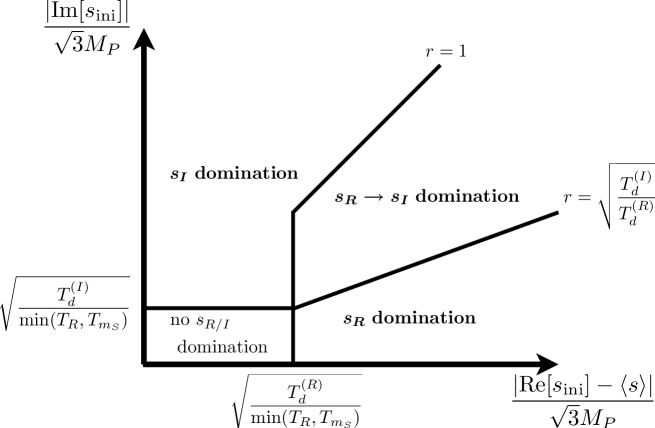
Figure 3: The condition of the $s$-dominated Universe.

As we will see in the next section, $T_{d}^{(I)}$ is always smaller than or equal to $T_{d}^{(R)}$. The history of the Universe depends on the values of the decay temperatures and $r$. There are four possibilities (cf Fig. 3):

Case 1: [$s_{I}$-domination] For $r>1$, the energy density of $s_{R}$ is always smaller than that of $s_{I}$, irrespective of whether (20) is satisfied or not. The $s_{I}$ dominates the energy of the Universe, if (21) is satisfied.

Case 2: [$s_{I}$-domination after $s_{R}$-domination] If (20) is satisfied for $\sqrt{T_{d}^{(I)}/T_{d}^{(R)}}<r<1$, it is $s_{R}$ that dominates the energy of the Universe first, and the $s_{I}$ dominates the energy of the Universe after the decay of $s_{R}$.

Case 3: [$s_{R}$-domination] If (20) is satisfied for $r<\sqrt{T_{d}^{(I)}/T_{d}^{(R)}}(<1)$, $s_{R}$ dominates the energy of the Universe, while $s_{I}$ does not.

Case 4: [$s_{I}$-domination] If (20) is not satisfied while (21) is satisfied for $r<1$, $s_{I}$ dominates the energy density of the Universe.

Once the energy density of the Universe is dominated by either $s_{R}$ or $s_{I}$, later discussions of the non-thermal gravitino production do not depend on the reheating temperature $T_{R}$. In Appendix B, we will consider the thermal effects, and a consistent parameter region for the $s$ domination is found to be $10^{-5}\lesssim\lambda\lesssim 10^{-3}$, $0.2\lesssim\theta\leq\pi/2$, and $10^{5}~{}{\rm GeV}\lesssim T_{R}\lesssim 10^{6}~{}{\rm GeV}$ for the set of reference values: $m_{3/2}=30~{}{\rm MeV}$, $m_{\tilde{B}}=200~{}{\rm GeV}$, $m_{S}=100~{}{\rm GeV}$ and $N=1$. We would like to emphasize here that the consistent ranges for $\lambda$ and $\theta$ depend on the choice of $m_{3/2}$, $m_{\tilde{B}}$ and $m_{S}$. For instance, the lowest allowed value of $\theta$ can be as small as ${\cal O}(0.01)$.

4 Decays of the $s$ field

The $s$ field mainly decays into the MSSM particles through loop diagrams of the messenger fields. We first discuss the main decay mode and calculate the decay temperatures.

4.1 Decays of $s_{R}$

The effective couplings between $s_{R}$ and the MSSM fields can be read off from the $\langle s\rangle$ dependencies of low-energy parameters. For scalar fields, the interaction terms are given by

$${\cal L}_{\rm int}^{(\tilde{f})}={\sqrt{2}(m_{\rm eff}^{(\tilde{f})})^{2}\over|\langle s\rangle|}\cdot s_{R}|\tilde{f}|^{2}.$$ (23)

The effective mass parameter $(m_{\rm eff}^{(\tilde{f})})^{2}$ is a part of the scalar mass that is proportional to $1/|\langle s\rangle|^{2}$, i.e., $(m_{\rm eff}^{(\tilde{f})})^{2}=-dm_{\tilde{f}}^{2}/d\log|\langle s\rangle|^{2}$. If gauge mediation is the only contribution to the scalar masses, $m_{\rm eff}^{(\tilde{f})}$ is identical to their masses. In realistic models of gauge mediation, the $\mu$ parameter needs to be generated by some mechanism, and such contributions to the masses of the Higgs fields may be independent of $\langle s\rangle$.

The couplings to the gauginos, $\lambda$, are

$${\cal L}_{\rm int}^{(\lambda)}={m_{\lambda}\over\sqrt{2}\langle s\rangle}\cdot{1\over 2}s_{R}\bar{\lambda}\lambda,$$ (24)

where $m_{\lambda}$ is the gaugino mass (cf. Eq. (4)). There is a similar coupling between $s_{R}$ to Higgsinos:

$${\cal L}_{\rm int}^{(\rm Higgsino)}=-{\mu_{\rm eff}\over\sqrt{2}\langle s\rangle}\cdot s_{R}\left(\overline{h_{d}^{c}}\cdot P_{L}h_{u}\right)+{\rm h.c.}$$ (25)

The coefficient $\mu_{\rm eff}$ is again a part of $\mu$ that is proportional to $1/\langle s\rangle$.

There are couplings to the quarks and leptons through a mixing between $s_{R}$ and Higgs bosons ($h^{0}$ and $H^{0}$). The mixing is induced through the interaction term in Eq. (23) for $\tilde{f}=H_{u},H_{d}$ with one of the Higgs fields replaced by its vacuum expectation value.

The couplings to the gauge bosons are

$${\cal L}_{\rm int}^{(A)}={1\over\sqrt{2}}{2g^{2}_{A}N\over(4\pi)^{2}}{1\over\langle s\rangle}\cdot{1\over 4}s_{R}F^{\mu\nu}_{(A)}F_{(A)\mu\nu},$$ (26)

where the index $A$ represents the gauge group (SU(3), SU(2), and U(1)).

The main decay mode of $s_{R}$ depends on the mass spectrum of SUSY particles. We discuss the case of the sweet spot SUSY model [33] in detail as an example of realistic models. In this model, the $\mu$-parameter and the Higgs soft masses are generated at the GUT scale through direct couplings between the Higgs fields and the SUSY breaking sector. Those contributions do not depend on $\langle s\rangle$. Additional large contributions to the $H_{u}$ soft mass are generated through gauge mediation and the renormalization group (RG) running. In particular, there is a significant RG effect due to the large Yukawa coupling of the top quark and the large scalar top masses. These contributions are proportional to $1/|\langle s\rangle|^{2}$, and thus enhance the effective coupling to $s_{R}$. The effective mass parameter $(m_{\rm eff}^{(H_{u})})^{2}$ is estimated to be

$$-(m_{\rm eff}^{(H_{u})})^{2}=(\kappa m_{\tilde{B}})^{2},$$ (27)

with

$$\kappa\simeq 3-4.$$ (28)

The parameter $\kappa$ depends logarithmically on the messenger scale. For the down type Higgs,

$$|(m_{\rm eff}^{(H_{d})})^{2}|\ll|(m_{\rm eff}^{(H_{u})})^{2}|,$$ (29)

due to relatively small RG effects. The effective coupling to the Higgsinos is also suppressed,

$$|\mu_{\rm eff}|\ll|\mu|,$$ (30)

in this model.

The enhancement in Eq. (28) is very important since there is no such factor in the $s_{I}$ decay. The decay modes $s_{R}\to hh$, $ZZ$, and $WW$ (where the gauge bosons are longitudinally polarized) and also the fermion modes such as $s_{R}\to b\bar{b}$ through the $s_{R}$-$h^{0}$ mixing are enhanced. This makes the $s_{R}$ decay much faster than that of $s_{I}$ in the parameter region of our interest.

The partial decay width of the $hh+WW+ZZ$ mode is given by

$$\Gamma_{s_{R}\to hh}+\Gamma_{s_{R}\to ZZ}+\Gamma_{s_{R}\to WW}\simeq{1\over 8\pi m_{S}}\left({\sqrt{2}(m_{\rm eff}^{(H_{u})})^{2}\sin^{2}\beta\over\langle s\rangle}\right)^{2}.$$ (31)

We ignored the mass differences among $h$, $Z$ and $W$, and also ${\cal O}(m_{h}^{2}/m_{S}^{2})$ and ${\cal O}(m_{h}^{2}/m_{A}^{2})$ terms for simplicity. The angle $\beta$ is defined by $\tan\beta=\langle H_{u}\rangle/\langle H_{d}\rangle$, and $m_{A}$ is the mass of the pseudo-scalar Higgs boson. If $s_{R}$ mainly decays into $hh+WW+ZZ$, the decay temperature $T_{d}^{(R)}$ is given by

$$T_{d}^{(R)} \simeq 13{\rm\,\,GeV}\,\cdot N^{-1}\left(\frac{g_{*}}{15}\right)^{-1/4}\left(\frac{m_{\rm eff}^{(H_{u})}}{800{\rm\,GeV}}\right)^{2}\left(\frac{m_{S}}{500{\rm\,GeV}}\right)^{-1/2}\left(\frac{m_{3/2}}{30{\rm\,MeV}}\right)^{-1}$$ (32)

$$\times\left(\frac{m_{\tilde{B}}}{200{\rm\,GeV}}\right)\,\sin^{2}\beta,$$

where we have defined the decay temperature as

$$T_{d}^{(R)}\;\equiv\;\left(\frac{\pi^{2}g_{*}}{90}\right)^{-1/4}\sqrt{\Gamma_{s_{R}}M_{\rm Pl}}.$$ (33)

In the numerical calculations below, we have included the phase space factors and contributions from other decay modes such as $t\bar{t}$.

The width of the $b\bar{b}$ mode through the mixing to the lightest Higgs boson is given by

$$\Gamma_{s_{R}\to b\bar{b}}\simeq{3m_{S}\over 8\pi}\left({\sqrt{2}(m_{\rm eff}^{(H_{u})})^{2}\sin^{2}\beta\over\langle s\rangle}\cdot{m_{b}\over m_{h}^{2}-m_{S}^{2}}\right)^{2}.$$ (34)

Correction terms of ${\cal O}(m_{b}^{2}/m_{S}^{2})$ are ignored. When the $b\bar{b}$ mode is dominant, the decay temperature is given by

$$T_{d}^{(R)} \simeq 1.6{\rm\,\,GeV}\,\cdot N^{-1}\left(\frac{g_{*}}{15}\right)^{-1/4}\left(\frac{m_{\rm eff}^{(H_{u})}}{800{\rm\,GeV}}\right)^{2}\left(\frac{m_{h}}{115{\rm\,GeV}}\right)^{-2}\left(\frac{m_{S}}{100{\rm\,GeV}}\right)^{1/2}$$ (35)

$$\times\left(\frac{m_{3/2}}{30{\rm\,MeV}}\right)^{-1}\left(\frac{m_{\tilde{B}}}{200{\rm\,GeV}}\right)\left|1-\frac{m_{S}^{2}}{m_{h}^{2}}\right|^{-1}\,\sin^{2}\beta.$$

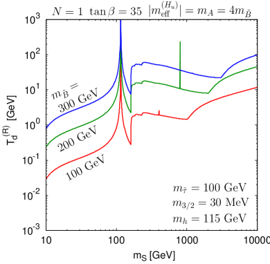
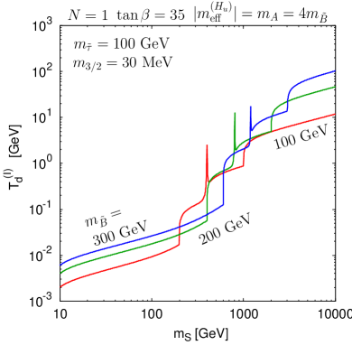
Figure 4: The decay temperatures of $s_{R}$ and $s_{I}$. We fixed the gravitino mass to be 30 MeV. For other values of $m_{3/2}$, the decay temperatures are obtained by multiplying $(m_{3/2}/30~{}{\rm MeV})^{-1}$.

We show in the left panel of Fig. 4 the decay temperature $T_{d}^{(R)}$ as a function of $m_{S}$ for $m_{\tilde{B}}=100$, 200, 300 GeV. In the figure, we fixed the gravitino mass to be 30 MeV. The decay temperatures for other values of $m_{3/2}$ can be obtained by multiplying a factor of $(m_{3/2}/30~{}{\rm MeV})^{-1}$. We have fixed other parameters to be $N=1$, $\tan\beta=35$, $m_{h}=115$ GeV and $|m_{\rm eff}^{(H_{u})}|=m_{A}=4m_{\tilde{B}}$, where $m_{A}$ is the pseudo-scalar Higgs boson mass. In the calculation, we have included the decay modes $s_{R}\to hh,ZZ,WW,\gamma\gamma,\widetilde{B}\widetilde{B},\widetilde{W}\widetilde{W},\tilde{g}\tilde{g},t\bar{t},b\bar{b},\tau\tau,\tilde{\tau}\tilde{\tau},gg$. The main decay mode of $s_{R}$ is $s_{R}\to hh,WW,ZZ$ for $2m_{W}<m_{S}\lesssim 1$ TeV. The gaugino modes become important for $m_{S}\gtrsim 1$ TeV. For $m_{S}<2m_{W}$, the $s_{R}\to b\bar{b}$ decay through the $s_{R}$-$h$ mixing is the main decay process. We can see a sharp peak at $m_{S}=m_{h}$ due to the enhancement of the mixing.

4.2 Decays of $s_{I}$

In Ref. [32], the decay property of $s_{I}$ is assumed to be the same as the one of $s_{R}$. We show in this subsection that the decay of $s_{I}$ happens much later in particular when $s_{R}\to hh$ is open. The difference of the decay temperatures will be important in calculating the non-thermal gravitino abundance.

The imaginary part, $s_{I}$, can only couple to CP-odd combinations. The enhanced coupling to Higgs bosons through a large value of $m_{\rm eff}^{(H_{u})}$ is therefore absent. There is a coupling to the Higgs bosons through an $\langle s\rangle$ dependence of the $B\mu$-term:

$${\cal L}\ni B\mu H_{u}H_{d}+{\rm h.c.},\to{i\over 2\sqrt{2}}{m_{A}^{2}\sin 2\beta\over\langle s\rangle}s_{I}H_{u}H_{d}+{\rm h.c.}$$ (36)

Here we have assumed $B\mu\propto\langle s\rangle^{-1}$ and used a tree-level relation from electroweak symmetry breaking, $B\mu=-(m_{A}^{2}\sin 2\beta)/2$. The coupling constant is suppressed by a $\sin 2\beta$ factor which is generically small in gauge-mediation models.

The decay into two gauginos is therefore important if it is kinematically open. The interaction Lagrangian is given by

$${\cal L}_{\rm int}\ni{1\over\sqrt{2}}{m_{\lambda}\over\langle s\rangle}\cdot{1\over 2}s_{I}\bar{\lambda}i\gamma_{5}\lambda.$$ (37)

Since this is the same strength as the $s_{R}\bar{\lambda}\lambda$ coupling, the lifetime of $s_{I}$ is always longer than $s_{R}$ due to the suppression of the Higgs modes. The partial decay width of the Bino mode is given by

$$\Gamma_{s_{I}\to\tilde{B}\tilde{B}}={m_{S}\over 32\pi}\left(m_{\tilde{B}}\over\langle s\rangle\right)^{2}\left(1-{4m_{\tilde{B}}^{2}\over m_{S}^{2}}\right)^{1/2}.$$ (38)

If this is the dominant decay channel, the decay temperature is given by

$$T_{d}^{(I)} \simeq 720~{}{\rm MeV}\cdot N^{-1}\left(g_{*}\over 15\right)^{-1/4}\left(m_{S}\over 500~{}{\rm GeV}\right)^{1/2}\left(m_{3/2}\over 30~{}{\rm MeV}\right)^{-1}\left(m_{\tilde{B}}\over 200~{}{\rm GeV}\right)^{2}$$ (39)

$$\times\left(1-{4m_{\tilde{B}}^{2}\over m_{S}^{2}}\right)^{1/4},$$

where the decay temperature is defined in the same way as (33). The Binos subsequently decay into staus if $m_{\tilde{B}}>m_{\tilde{\tau}}$. In a large $m_{S}$ region, the Wino and the gluino modes become more important. However, as we will see later, such a region is not allowed because of the overproduction of gravitinos.

If the Bino mode is closed, the main decay mode is into $b\bar{b}$ through the $s_{I}$-$A^{0}$ mixing from Eq. (36). The partial width is calculated to be

$$\Gamma_{s_{I}\to b\bar{b}}={3m_{S}\over 16\pi}\left({m_{A}^{2}\sin^{2}\beta\over\langle s\rangle}\cdot{m_{b}\over m_{A}^{2}-m_{S}^{2}}\right)^{2}.$$ (40)

When the $b\bar{b}$ mode is dominant, the decay temperature is

$$T_{d}^{(I)} \simeq 16~{}{\rm MeV}\cdot N^{-1}\left({g_{*}\over 15}\right)^{-1/4}\left(m_{S}\over 100~{}{\rm GeV}\right)^{1/2}\left(m_{3/2}\over 30~{}{\rm MeV}\right)^{-1}\left(m_{\tilde{B}}\over 200~{}{\rm GeV}\right)$$ (41)

$$\times\left|1-{m_{S}^{2}\over m_{A}^{2}}\right|^{-1}\sin^{2}\beta.$$

The value in front becomes 18 MeV once we include the $\tau\tau$ mode.

The decay temperature as a function of $m_{S}$ is shown in the right panel of Fig. 4. We have used a set of parameters which are indicated in the figure. Again, for other values of $m_{3/2}$, $T_{d}^{(I)}\propto m_{3/2}^{-1}$. As we can see, $T_{d}^{(I)}$ is significantly lower than $T_{d}^{(R)}$ for $m_{S}\lesssim 1$ TeV. The decay modes $s_{I}\to\widetilde{B}\widetilde{B},\widetilde{W}\widetilde{W},\tilde{g}\tilde{g},t\bar{t},b\bar{b},\tau\tau,gg,\gamma\gamma,hA,HZ$ are included in the calculation. We have ignored the $hZ$ mode because it is much smaller than the $b{\bar{b}}$ mode. The gauge invariance requires the $hZ$ mode to vanish in the decoupling limit, $m_{h}/m_{A}\to 0$.

5 Non-thermal gravitino production

The $s$ field can decay into two gravitinos with a suppressed branching fraction. We calculate here the branching ratio and estimate the gravitino energy density. We will see that the non-thermal component can explain the DM abundance when $m_{S}\sim{\cal O}(100)$ GeV independent of the gravitino mass.

5.1 Abundance

The non-thermal gravitino abundance can be calculated from the decay temperatures and the branching ratios of the $s_{R,I}\to\psi_{3/2}\psi_{3/2}$ decays. The partial decay width of $s_{R,I}$ into two gravitinos, $s_{R,I}\to\psi_{3/2}\psi_{3/2}$, is given by [15, 16, 17, 32]

$$\Gamma_{3/2}={1\over 96\pi}{m_{S}^{3}\over M_{\rm Pl}^{2}}\left({m_{S}\over m_{3/2}}\right)^{2}.$$ (42)

This formula is obtained from the interaction term in the second term of Eq. (1) by identifying the fermion component of $S$ with the longitudinal mode of the gravitino. By using this partial decay width, we can calculate the branching fraction.

There are two interesting branches where the main decay modes are different. For the $s_{R}$ decay, the main decay mode is (A) $s_{R}\to b\bar{b}$ for $2m_{b}<m_{S}<2m_{W}$, and (B) $s_{R}\to hh,WW,ZZ$ for $2m_{W}<m_{S}\lesssim 1$ TeV. The branching ratios of the two-gravitino mode in those cases are respectively given by

$$B_{3/2}^{(R)} \simeq 4.6\times 10^{-9}\cdot N^{2}\left(|m_{\rm eff}^{(H_{u})}|\over 800~{}{\rm GeV}\right)^{-4}\left(m_{S}\over 100~{}{\rm GeV}\right)^{4}\left(m_{\tilde{B}}\over 200~{}{\rm GeV}\right)^{-2}\left(\frac{m_{h}}{115{\rm GeV}}\right)^{4}$$

$$\times\left(1-\frac{m_{S}^{2}}{m_{h}^{2}}\right)^{2}\sin^{-4}\beta\ \ \cdots\mbox{(A)},$$

$$B_{3/2}^{(R)}\simeq 2.2\times 10^{-7}\cdot N^{2}\left(|m_{\rm eff}^{(H_{u})}|\over 800~{}{\rm GeV}\right)^{-4}\left(m_{S}\over 500~{}{\rm GeV}\right)^{6}\left(m_{\tilde{B}}\over 200~{}{\rm GeV}\right)^{-2}\sin^{-4}\beta\ \cdots\mbox{(B)}.$$

It is interesting to notice that the branching ratio is independent of $m_{3/2}$. For the $s_{I}$ decay, the main decay mode is (C) $s_{I}\to b\bar{b}$ ($m_{S}<2m_{\tilde{B}}$) or (D) $s_{I}\to\widetilde{B}\widetilde{B}$ ($m_{S}>2m_{\tilde{B}}$). The branching ratios in two cases are

$$B_{3/2}^{(I)}\simeq 4.2\times 10^{-5}\cdot N^{2}\left(m_{S}\over 100~{}{\rm GeV}\right)^{4}\left(m_{\tilde{B}}\over 200~{}{\rm GeV}\right)^{-2}\left(1-{m_{S}^{2}\over m_{A}^{2}}\right)^{2}\sin^{-4}\beta\ \ \cdots\mbox{(C)},$$

$$B_{3/2}^{(I)}\simeq 7.2\times 10^{-5}\cdot N^{2}\left(m_{S}\over 500~{}{\rm GeV}\right)^{4}\left(m_{\tilde{B}}\over 200~{}{\rm GeV}\right)^{-4}\left(1-{4m_{\tilde{B}}^{2}\over m_{S}^{2}}\right)^{-1/2}\ \ \cdots\mbox{(D)}.$$

We here define quantities $\Omega_{3/2}^{(R)}$ and $\Omega_{3/2}^{(I)}$ which represent the density parameters of the gravitino when we ignore the presence of $s_{I}$ and $s_{R}$, respectively:

$$\Omega_{3/2}^{(R)} \equiv {3\over 4}{m_{3/2}}{T_{d}^{(R)}\over m_{S}}B_{3/2}^{(R)}\times 2\Big{/}(\rho_{c}/s)_{0},$$ (43)

$$\Omega_{3/2}^{(I)} \equiv {3\over 4}{m_{3/2}}{T_{d}^{(I)}\over m_{S}}B_{3/2}^{(I)}\times 2\Big{/}(\rho_{c}/s)_{0},$$ (44)

where $(\rho_{c}/s)_{0}\simeq 1.8\times 10^{-9}$ GeV is the critical density divided by the entropy density at present. The abundances $\Omega_{3/2}^{(R)}$ and $\Omega_{3/2}^{(I)}$ are related as

$${\Omega_{3/2}^{(R)}\over\Omega_{3/2}^{(I)}}={T_{d}^{(I)}\over T_{d}^{(R)}},$$ (45)

where we used the fact that $B_{3/2}^{(R)}/B_{3/2}^{(I)}=(T_{d}^{(I)}/T_{d}^{(R)})^{2}$. In the actual situation, of course, one cannot totally neglect $s_{R}$ or $s_{I}$, and one has to take into account both of the contributions and also the dilution effects. The gravitino abundance in a general case can be expressed in terms of $\Omega_{3/2}^{(R)}$ and $\Omega_{3/2}^{(I)}$ as

$$\Omega_{3/2}^{\rm NT}=\left\{\begin{array}[]{ll}\Omega_{3/2}^{(R)}+r^{2}\Omega_{3/2}^{(I)}\left({\displaystyle{T_{d}^{(R)}\over T_{d}^{(I)}}}\right),&{\rm for~{}~{}}r<\displaystyle{\sqrt{T_{d}^{(I)}/T_{d}^{(R)}}}\\ r^{-2}\Omega_{3/2}^{(R)}\left({\displaystyle{T_{d}^{(I)}\over T_{d}^{(R)}}}\right)+\Omega_{3/2}^{(I)},&{\rm for~{}~{}}r>\displaystyle{\sqrt{T_{d}^{(I)}/T_{d}^{(R)}}}\end{array}\right..$$ (48)

The former and latter regions of $r$ respectively correspond to the cases where $s_{I}$ does not and does dominate the energy density of the Universe before the $s_{I}$ decays. For $r>T_{d}^{(I)}/T_{d}^{(R)}$, most of the gravitinos are produced by the $s_{I}$ decay. For $r^{2}>T_{d}^{(I)}/T_{d}^{(R)}$, both radiation and gravitinos arise from the $s_{I}$ decay, and thus the gravitino abundance becomes insensitive to $r$. Note that $\Omega_{3/2}^{(R)}$ ($\Omega_{3/2}^{(I)}$) corresponds to the gravitino density parameter in the limit of $r\rightarrow 0$ ($r\rightarrow\infty$).

Since $T_{d}^{(R,I)}\propto 1/\langle s\rangle\propto m_{3/2}^{-1}$ and the branching fractions $B_{3/2}^{(R,I)}$ are independent of $m_{3/2}$, both $\Omega_{3/2}^{(R)}$ and $\Omega_{3/2}^{(I)}$ are also independent of the gravitino mass. Therefore, interestingly, the total gravitino energy density $\Omega_{3/2}^{\rm NT}$ does not depend on the gravitino mass.

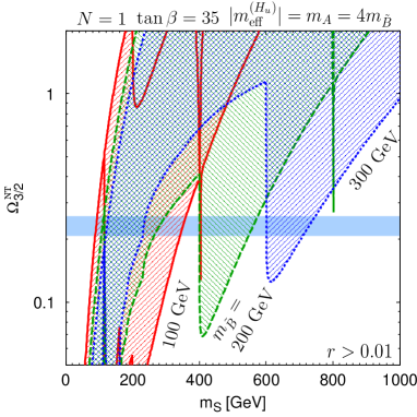
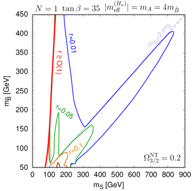
Figure 5: The non-thermal gravitino abundance with respect to $m_{S}$ for several values of the Bino mass $m_{\tilde{B}}=100,200$, and $300$ GeV (Left). We have varied $r$ from $0.01$ to ${\cal O}(1)$ for each value of $m_{\tilde{B}}$. The other parameters are shown above the panel. For $r\gtrsim 1$, the three regions overlap one another around $m_{S}\sim 100$ GeV and $m_{\tilde{B}}>100$ GeV. The right panel shows the contours of $\Omega_{3/2}^{\rm NT}=0.2$ for various values of $r$. For $r\gtrsim{\cal O}(0.1)$, the abundance does not depend on $r$ since the $s_{I}$ oscillation dominates over the Universe. The gravitino abundance becomes larger as $m_{S}$ increases (see Eq. (49)).

We show in the left panel of Fig. 5 the gravitino abundance for fixed values of $m_{\tilde{B}}$ for $r>0.01$. The non-thermal gravitino can account for the observed DM abundance for $m_{S}={\cal O}(100)$ GeV. In the right panel, contours of $\Omega_{3/2}^{\rm NT}=0.2$ for various values of $r$ are shown on the $m_{S}$-$m_{\tilde{B}}$ plane. For $r\gtrsim{\cal O}(0.1)$, the contour gets independent of $r$ for $m_{\tilde{B}}>100$ GeV. For $r\gtrsim 0.05$, the correct abundance is obtained for $m_{S}\sim 100$ GeV where $s_{I}\to b\bar{b}$ is the dominant decay mode. The gravitino abundance for that case is given by

$$\Omega^{\rm NT}_{3/2}\simeq 0.2\cdot N\left(m_{S}\over 100~{}{\rm GeV}\right)^{7/2}\left(m_{\tilde{B}}\over 200~{}{\rm GeV}\right)^{-1}.$$ (49)

The abundance does not depend on the detailed model parameters such as $\kappa$, $m_{A}$ or $\tan\beta$ as long as $m_{A}\gg m_{S}$ and $\tan\beta\gtrsim 3$. In general, this result applies to models where the $B\mu$-term is proportional to $\langle s\rangle^{-1}$ and the decay width in Eq. (34) is larger than or comparable to that in Eq. (40).

Although the abundance is independent of $m_{3/2}$, the gravitino mass cannot be arbitrarily large. In order to avoid overproduction of ⁴He, the decay temperature of $s_{I}$ is required to be higher than $\sim 10$ MeV [39], which gives an upper bound on the gravitino mass. For $m_{S}=100$ GeV and $m_{\tilde{B}}\gtrsim 100$ GeV with $r\gtrsim 0.05$ motivated by DM abundance, we obtain from Eq. (41):

$$m_{3/2}\;\lesssim\;{\cal O}(100)~{}{\rm MeV}.$$ (50)

If one allows a small value of $r$, there is a region where $s_{I}\to\tilde{B}\tilde{B}$ is open while $\Omega_{3/2}^{\rm total}=0.2$ is satisfied. The upper bound on the gravitino mass in this case is relaxed to ${\cal O}(1)$ GeV. Such a region is subject to the BBN constraint from the decay of the non-thermally produced NLSP. We will discuss the constraint later in the Appendix C.

5.2 Thermal component

Here we comment on the amount of thermally produced gravitinos. After accounting for the dilution effect by the entropy production of the $s$ decays, the density parameter of the thermally produced gravitinos is estimated to be [32]

$$\Omega_{3/2}^{\rm th} \simeq 0.004\left({m_{3/2}\over 30~{}{\rm MeV}}\right)^{-1}\left({m_{\tilde{B}}\over 200~{}{\rm GeV}}\right)^{2}\left({T_{d}\over 18~{}{\rm MeV}}\right)\left({|s_{\rm ini}|\over 2.5\times 10^{15}~{}{\rm GeV}}\right)^{-2},$$ (51)

where $|s_{\rm ini}|$ is the size of the initial amplitude. If the entropy of the Universe is generated by the decay of $s_{R}$ ($s_{I}$), one should substitute $T_{d}^{(R)}$ ($T_{d}^{(I)}$) for $T_{d}$. This expression is independent of the reheating temperature after inflation even though most of the gravitinos are produced at the end of the reheating process.

Let us assume that $s_{I}$ dominates the energy density of the Universe. In the case where the $s_{I}\to b\bar{b}$ mode is the dominant decay process, we obtain

$$\Omega_{3/2}^{\rm th} \simeq 0.004\cdot N^{-1}\left({m_{S}\over 100~{}{\rm GeV}}\right)^{5/2}\left({m_{3/2}\over 30~{}{\rm MeV}}\right)^{-4}\left({m_{\tilde{B}}\over 200~{}{\rm GeV}}\right)^{3}\left({|s_{\rm ini}|\over\Lambda}\right)^{-2},$$ (52)

where $\Lambda$ is the cut-off scale in Eq. (1). The $|s_{\rm ini}|/\Lambda$ factor cannot exceed ${\cal O}(1)$ for the discussion to be within the framework of the effective theory. In order for the thermal component not to exceed the observed DM density of the Universe, we obtain a lower limit of the gravitino mass:

$$m_{3/2}\;\gtrsim\;{\cal O}(10)~{}{\rm MeV},$$ (53)

for $m_{S}\sim 100$ GeV and $m_{\tilde{B}}\sim 200$ GeV.

On the other hand, if $s_{I}\to{\tilde{B}}{\tilde{B}}$ mode is open, the gravitino abundance becomes

$$\Omega_{3/2}^{\rm th} = 0.1\cdot N^{-1}\left({m_{S}\over 500~{}{\rm GeV}}\right)^{5/2}\left({m_{3/2}\over 100~{}{\rm MeV}}\right)^{-4}\left({m_{\tilde{B}}\over 200~{}{\rm GeV}}\right)^{4}$$ (54)

$$\times\left({|s_{\rm ini}|\over\Lambda}\right)^{-2}\left(1-{4m_{\tilde{B}}^{2}\over m_{S}^{2}}\right)^{1/4}.$$

The gravitino mass must be slightly heavier than the previous case,

$$m_{3/2}\gtrsim{\cal O}(100)~{}{\rm MeV},$$ (55)

for $m_{S}\sim 500$ GeV and $m_{\tilde{B}}\sim 200$ GeV.

5.3 Free-streaming scale

We have seen that the gravitinos non-thermally produced by the decay of $s$ successfully account for the observed abundance of DM. Since the gravitinos are relativistic at the production, we need to check if the free-streaming scale is consistent with the observational bound, $\lambda_{FS}\lesssim{\cal O}(100)$ kpc, from the Lyman $\alpha$ forest data [40].

Let us first derive an expression for the free-steaming length, $\lambda_{FS}$, which is a distance that particles (gravitinos in our case) can travel until they become non-relativistic. In the following the gravitinos are assumed to be produced by the decay of $s$ (either $s_{R}$ or $s_{I}$), and the decay temperature $T_{d}$ denotes either $T_{d}^{(R)}$ or $T_{d}^{(I)}$. Let us denote by $p$ the momentum of the gravitino. Due to the cosmic expansion, the momentum red-shifts as $p\propto a^{-1}$, where $a$ denotes the scale factor. Noting that the velocity of a particle is given by the ratio of the momentum to the energy, the free-streaming length is expressed as

$$\lambda_{FS} = \int_{a_{d}}^{a_{eq}}\frac{p_{d}\left(\frac{a_{d}}{a}\right)}{\sqrt{m_{3/2}^{2}+p_{d}^{2}\left(\frac{a_{d}}{a}\right)^{2}}}\frac{1}{a}\left(\frac{dt}{da}\right)da,$$ (56)

where $p_{d}$ is the initial momentum at the production, $a_{d}$ and $a_{eq}$ are the scale factors at the decay of $s$ and at the matter-radiation equality, respectively, and the scale factor is normalized to be unity at present. We take the matter-radiation equality as the end point of integration, assuming that the gravitino has become already non-relativistic at the equality. The assumption is satisfied for the whole parameter space of interest.

Assuming that the Universe was radiation dominated since the gravitino production until the equality, we can perform the integration and obtain

$$\lambda_{FS} \simeq \frac{1+z_{eq}}{H_{eq}}\left(\frac{m_{S}}{2m_{3/2}}\frac{a_{d}}{a_{eq}}\right)\sinh^{-1}\left(\frac{2m_{3/2}}{m_{S}}\frac{a_{eq}}{a_{d}}\right),$$ (57)

$$\simeq 60{\rm\,kpc}\left(\frac{g_{*}}{15}\right)^{-\frac{1}{4}}\left(\frac{m_{3/2}}{30{\rm\,MeV}}\right)^{-1}\left(\frac{m_{S}}{100{\rm\,GeV}}\right)\left(\frac{T_{d}}{18{\rm\,MeV}}\right)^{-1}$$

$$\times\left\{1-0.1\ln\left[\left(\frac{g_{*}}{15}\right)^{-\frac{1}{4}}\left(\frac{m_{3/2}}{30{\rm\,MeV}}\right)^{-1}\left(\frac{m_{S}}{100{\rm\,GeV}}\right)\left(\frac{T_{d}}{18{\rm\,MeV}}\right)^{-1}\right]\right\},$$

where $z_{eq}$ and $H_{eq}$ are the red-shift and the Hubble parameter at the equality, respectively, and we have adopted an approximation, $m_{S}\gg m_{3/2}$. In the last equality, we have used $z_{eq}\simeq 3176$ and $H_{eq}\simeq 31\,{\rm Mpc}^{-1}$ [1].

If the decay of $s$ produces not only the gravitinos but also the (almost) entire entropy of the Universe, we can express the free-streaming length in terms of the branching fraction of the gravitino production. The free-streaming length is then give by

$$\lambda_{FS} \simeq 60{\rm\,kpc}\left(\frac{g_{*}}{15}\right)^{-\frac{1}{4}}\left(\frac{\Omega_{3/2}^{\rm NT}}{0.2}\right)^{-1}\left(\frac{B_{3/2}}{4\times 10^{-5}}\right)$$ (58)

$$\times\left\{1-0.1\ln\left[\left(\frac{g_{*}}{15}\right)^{-\frac{1}{4}}\left(\frac{\Omega_{3/2}^{\rm NT}}{0.2}\right)^{-1}\left(\frac{B_{3/2}}{4\times 10^{-5}}\right)\right]\right\}.$$

Since $B_{3/2}$ is independent of $m_{3/2}$, the free-streaming scale is also independent of $m_{3/2}$ once we fix the gravitino abundance. Note that the expression Eq. (58) is valid only for $r<T_{d}^{(I)}/T_{d}^{(R)}$ or $r>\sqrt{T_{d}^{(I)}/T_{d}^{(R)}}$, while Eq. (57) holds for any values of $r$ as long as the gravitino comes mainly from either $s_{R}$ or $s_{I}$. In the parameter region of our interest, where $s_{I}\to b\bar{b}$ is the main decay mode, the free-streaming scale is of ${\cal O}(100)$ kpc, which is on the border of the Lyman-$\alpha$ bound, $\lambda_{FS}\lesssim{\cal O}(100)$ kpc. It is an interesting possibility that we may be able to see the suppression of the structure formation below the corresponding scale.

5.4 Isocurvature perturbations

During inflation, $s$ is assumed to be at $|s_{\rm ini}|\sim\Lambda$, far deviated from the origin. If the $s$ field has an approximate U(1) symmetry, the phase component, $\theta\equiv{arg}[s]$, remains light and therefore acquires quantum fluctuations $\delta\theta=H_{I}/(2\pi|s_{\rm ini}|)$, where $H_{I}$ represents the Hubble parameter during inflation. The phase $\theta$ is related to $r$ (the ratio of the initial values of $s_{R}$ and $s_{I}$) as $\tan\theta=r$. Therefore, $\delta\theta$ amounts to the fluctuation $\delta r$, which generically leads to the isocurvature fluctuations in the gravitino DM. This is because $s_{R}$ and $s_{I}$ have different decay temperatures and different branching ratios into the gravitinos.

Recall that the gravitino abundance becomes insensitive to $r$ for $r\gg\sqrt{T_{d}^{(I)}/T_{d}^{(R)}}$. This is because both the radiation and the gravitino are produced mainly from the decay of $s_{I}$. Thus, the cold DM (CDM) isocurvature perturbation is also suppressed in this case [41]. Intuitively speaking, for a large enough value of $r$, we can simply neglect the $s_{R}$; the fluctuations in radiation and the gravitino DM are then adiabatic, since both are generated from a single source, $s_{I}$.

To see this more explicitly, let us estimate the CDM isocurvature perturbation $S_{c\gamma}$ in the case of $r\gg\sqrt{T_{d}^{(I)}/T_{d}^{(R)}}$. From Eqs. (45) and (48), we have

$${S_{c\gamma}\;\equiv\;\delta\left(\log\left(\frac{\rho_{3/2}}{s}\right)\right)\simeq-2\frac{1+r^{2}}{r^{3}}\left(\frac{T_{d}^{(I)}}{T_{d}^{(R)}}\right)^{2}}\frac{H_{I}}{2\pi|s_{\rm ini}|},$$ (59)

where we have used $\delta r=\delta\theta/\cos^{2}\theta$ in the last equality. As we mentioned above, we can see that $S_{c\gamma}$ is suppressed for $r\gg\sqrt{T_{d}^{(I)}/T_{d}^{(R)}}$. The current observation bound on the isocurvature perturbation reads $|S_{c\gamma}|\lesssim 2\times 10^{-5}$ at $95$%C.L. [1]. Thus, $H_{I}$ is bounded above not to exceed the current constraint on the isocurvature perturbation,

$$H_{I}\;\lesssim\;2\times 10^{11}{\rm\,GeV}\left(\frac{r^{3}}{1+r^{2}}\right)\left(\frac{T_{d}^{(R)}}{T_{d}^{(I)}}\right)^{2}\left(\frac{m_{3/2}}{30~{}{\rm MeV}}\right)\left(\frac{m_{S}}{100~{}{\rm GeV}}\right)^{-1}\left(\frac{|s_{\rm ini}|}{\Lambda}\right).$$ (60)

There are plentiful inflation models which satisfy the bound.

6 Sweet spot

We have seen that the non-thermal production of the gravitino can explain DM of the Universe in a class of gauge mediation models. For $r\gtrsim 0.05$, the correct abundance is obtained when the $s_{I}\to b\bar{b}$ mode is the dominant decay mode. The abundance in that case is given by Eq. (49) which is independent of $m_{3/2}$. The constraints from the thermal production of the gravitino (Eq. (53)) and the decay temperature (Eq. (50)) restrict the mass range of the gravitino to be

$$10~{}{\rm MeV}\lesssim m_{3/2}\lesssim 100~{}{\rm MeV}.$$ (61)

Interestingly, the above mass range and $m_{S}\sim 100~{}{\rm GeV}$ overlaps with the prediction of the gravitational stabilization mechanism in Ref. [35]. This model relates $\langle s\rangle$ and $\Lambda$ by

$$\langle s\rangle={\sqrt{3}\Lambda^{2}\over 6M_{\rm Pl}},$$ (62)

which is translated into a relation among $m_{S}$, $m_{3/2}$ and $m_{\tilde{B}}$ as

$$m_{3/2}=34~{}{\rm MeV}\cdot N\left(m_{S}\over 100~{}{\rm GeV}\right)^{2}\left(m_{\tilde{B}}\over 200~{}{\rm GeV}\right)^{-1}.$$ (63)

The reference value we took approximately satisfies the relation. It is also interesting to note that the above supergravity effect always exists. Therefore, there is no big room left for other mechanisms to give messenger masses in the scenario of the $s$-dominated Universe.

Ref. [33] proposed a solution to the $\mu$ problem by using the above gravitational stabilization mechanism. The $\mu$-term is generated from the direct interaction terms between the SUSY breaking sector and the Higgs fields, $K\ni S^{\dagger}H_{u}H_{d}/\Lambda$. This framework predicts

$$\mu\sim{F_{S}\over\Lambda}\sim m_{S},$$ (64)

which is perfectly consistent with $\mu\sim{\cal O}(100)$ GeV required from electroweak symmetry breaking and $m_{S}\sim{\cal O}(100)$ GeV from gravitino DM.

Appendix A Spatial instabilities

Let us estimate a condition for an instability to grow. The scalar potential of $s=(s_{R}+is_{I})/\sqrt{2}$ is given by

$$V(s_{R},s_{I})\;=\;\frac{1}{2}m_{S}^{2}\left((s_{R}-\sqrt{2}\langle s\rangle)^{2}+s_{I}^{2}\right)+\frac{5N}{16\pi^{2}}\lambda^{2}F_{S}^{2}\log\left(\frac{s_{R}^{2}+s_{I}^{2}}{2\Lambda^{2}}\right).$$ (65)

Differentiating the scalar potential with respect to $s_{R}$ and $s_{I}$, we obtain

$${\cal M}^{2} \equiv \left(\begin{array}[]{cc}\frac{\partial^{2}V}{\partial s_{R}^{2}}&\frac{\partial^{2}V}{\partial s_{R}\partial s_{I}}\\ \frac{\partial^{2}V}{\partial s_{R}\partial s_{I}}&\frac{\partial^{2}V}{\partial s_{I}^{2}}\\ \end{array}\right)$$ (68)

$$= {\displaystyle\left(\begin{array}[]{cc}m_{S}^{2}+\frac{5N}{16\pi^{2}}\lambda^{2}F_{S}^{2}\left(\frac{2}{s_{R}^{2}+s_{I}^{2}}-\frac{4s_{R}^{2}}{(s_{R}^{2}+s_{I}^{2})^{2}}\right)&-\frac{5N}{16\pi^{2}}\lambda^{2}F_{S}^{2}\frac{4s_{R}s_{I}}{(s_{R}^{2}+s_{I}^{2})^{2}}\\ -\frac{5N}{16\pi^{2}}\lambda^{2}F_{S}^{2}\frac{4s_{R}s_{I}}{(s_{R}^{2}+s_{I}^{2})^{2}}&m_{S}^{2}+\frac{5N}{16\pi^{2}}\lambda^{2}F_{S}^{2}\left(\frac{2}{s_{R}^{2}+s_{I}^{2}}-\frac{4s_{I}^{2}}{(s_{R}^{2}+s_{I}^{2})^{2}}\right)\end{array}\right)}$$ (71)

Neglecting the cosmic expansion, the instability grows if ${\rm det}[{\cal M}^{2}]<0$. Thus, the condition for the instabilities not to grow is ${\rm det}[{\cal M}^{2}]>0$, namely

$$|s|^{2}>\frac{5N}{16\pi^{2}m_{S}^{2}}\lambda^{2}F_{S}^{2}=\left(\frac{\lambda}{\lambda_{\rm max}}\right)^{2}\frac{\langle s\rangle^{2}}{4},$$ (73)

or equivalently,

$$\lambda\;<\;2\lambda_{\rm max}\sin\theta.$$ (74)

Appendix B Remarks on initial conditions

In this Appendix, we discuss conditions for $s_{R,I}$ to dominate the energy density of the Universe, taking account of finite temperature effects. For concreteness, we set $m_{3/2}\simeq 30~{}{\rm MeV}$, $m_{\tilde{B}}\simeq 200~{}{\rm GeV}$, $m_{S}\simeq 100~{}{\rm GeV}$ and $N=1$, and also $r\gtrsim{\cal O}(1)$ as reference values, which lead to a successful gravitino DM scenario from the $s_{I}$ decay, as discussed in the text. Therefore we are concerned with a condition for $s_{I}$ to dominate the energy density of the Universe.

B.1 $s_{I}$-domination

The $s_{I}$-domination condition Eq. (21) leads to

$$\left|{\rm Im}[s_{\rm ini}]\right| \gtrsim 7\times 10^{12}{\rm\,GeV}\cdot\left(\frac{{\rm min}[T_{R},T_{m_{S}}]}{7\times 10^{9}{\rm\,GeV}}\right)^{-1/2}\left(\frac{T_{d}^{(I)}}{18\,{\rm MeV}}\right)^{1/2}.$$ (75)

If we take a natural expectation, $|s_{\rm ini}|\sim\Lambda$, the $s_{I}$ domination can be realized for $T_{R}\gtrsim 10^{5}{\rm\,GeV}$.

B.2 Finite temperature effects

In this subsection, we assume that the $s$ field starts its oscillations when the Universe is dominated by the oscillating inflaton. Even before the reheating, however, there is a background dilute plasma with a temperature $T\simeq(T_{R}^{2}M_{\rm Pl}H)^{1/4}$. The potential of $s$ field therefore receives thermal corrections, which are not taken into consideration so far. Here we briefly discuss the finite temperature effects on the evolution of the $s$ field and the messenger fields.

There are two thermal effects on the $s$ field: thermal mass and thermal logarithmic terms, which arise depending on whether the messenger fields are in thermal bath or not. If the effective masses of the messenger fields are smaller than the temperature of thermal plasma, i.e., $m_{\rm eff}=\lambda|s|<T$, the messenger fields will be in thermal equilibrium. The $s$ field then receives a thermal mass:

$$V_{T}^{(1)}\;=\;\frac{5}{4}N\lambda^{2}T^{2}|S|^{2}~{}~{}~{}~{}~{}~{}~{}{\rm for~{}~{}}\lambda|s|<T,$$ (76)

where we have assumed that the messenger fields transform as ${\bf 5}$ and $\bf{\bar{5}}$ under SU(5).

On the other hand, when the messenger fields are so heavy that they are decoupled from thermal bath, there is a thermal effect arising from the two-loop contribution to the free energy, $\delta V\propto g(T)^{2}T^{4}$. Here we consider only the SU(3)_C gauge group, which gives the dominant contribution to the free energy [42],

$$\delta V\;=\;\frac{21}{8}g_{3}^{2}(T)T^{4}.$$ (77)

For $\lambda|s|>T$, the running gauge coupling $g_{3}(T)$ is modified as

$$g_{3}(T)|_{\lambda|s|>T} = g_{3}(T)|_{s=\langle s\rangle}+N\frac{g_{3}(M_{U})^{3}}{32\pi^{2}}\ln\left(\frac{\lambda^{2}|s|^{2}}{T^{2}}\right),$$ (78)

where $M_{U}$ is some ultraviolet scale where $g_{3}$ is fixed. This leads to a thermal correction to the scalar potential

$$V_{T}^{(2)} = \frac{21N}{8}\alpha_{3}(T)^{2}T^{4}\ln\left(\frac{|s|^{2}}{T^{2}}\right)~{}~{}~{}~{}~{}~{}~{}{\rm for~{}~{}}\lambda|s|>T,$$ (79)

which may become important where the thermal mass term is negligible.

Next let us consider the thermal effect on the messenger fields. The messenger fields acquire thermal masses through the gauge interactions with the SSM particles in thermal plasma. The thermal masses tend to prevent the messengers from falling into a SUSY minimum. In principle this effect could enlarge the allowed region for $r$: even with a small value of $r$, the messengers may be stabilized at their origin and the $s$ field may settle down at the SUSY breaking minimum in the end. However, if this is the case, our scenario would be modified in two ways. First, the messenger fields are in thermal equilibrium when they are stabilized by their thermal masses. If the messenger number is conserved, the lightest messenger may exceed the DM abundance. Although this issue can be avoided by introducing the breaking of the messenger number, it would make the analysis model-dependent. Second, the gravitino abundance (51) is modified because the gravitinos are also generated from the scattering processes including messengers [43]. Thus, in order to keep the success of our scenario in the text, we assume that the messenger fields are so heavy that they are always decoupled from thermal plasma.

We have shown in Fig. 6 a parameter space in which (i) the perturbation $\delta s$ remains small compared to ${\bar{s}}$ until the $s$ field is stabilized at the SUSY breaking minimum and (ii) the messengers remain decoupled from thermal bath during the course of evolution, for $T_{R}=10^{5}{\rm\,GeV}$ and $10^{6}{\rm\,GeV}$ with the thermal effects (76) and (79) taken into account. Here we have set $m_{3/2}=30~{}{\rm MeV}$, $m_{\tilde{B}}=200~{}{\rm GeV}$, $m_{S}=100~{}{\rm GeV}$ and $N=1$. Notice that, compared to the zero-temperature result shown in Fig. 2, smaller values of $\lambda$ are excluded since the messengers would be thermalized. The allowed region disappears for $T_{R}>10^{7}{\rm\,GeV}$. Therefore, our scenario works for $10^{-5}\lesssim\lambda\lesssim 10^{-3}$, $0.2\lesssim\theta\leq\pi/2$ and $10^{5}{\rm\,GeV}\lesssim T_{R}\lesssim 10^{6}{\rm\,GeV}$, if thermal effects are taken into account. Note that the consistent ranges for $\lambda$ and $\theta$ depend on the choice of $m_{3/2}$, $m_{\tilde{B}}$ and $m_{S}$. For instance, the lowest allowed value of $\theta$ can be as small as ${\cal O}(0.01)$ for e.g. $m_{S}=400$ GeV and $m_{\tilde{B}}=100$ GeV.

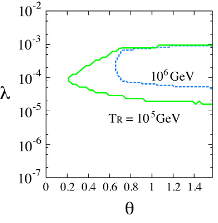
Figure 6: The parameter region where the $s$ field is trapped by the SUSY breaking minimum and the messenger fields are decoupled from the thermal bath, when the thermal effects (76) and (79) are taken into account. We have set $m_{3/2}=30~{}{\rm MeV}$, $m_{\tilde{B}}=200~{}{\rm GeV}$, $m_{S}=100~{}{\rm GeV}$ and $N=1$.

Appendix C BBN constraints

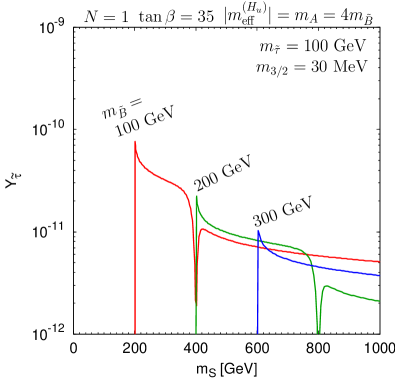
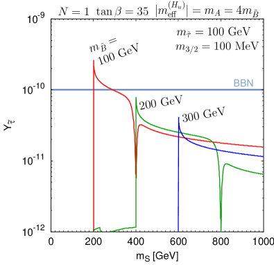
Figure 7: The abundance of the non-thermally produced staus. We took $m_{\tilde{\tau}}=100$ GeV. The gravitino mass is $m_{3/2}=30$ MeV (left) and 100 MeV (right). The abundance is inversely proportional to the decay temperature.

If the decay of $s_{R}$ or $s_{I}$ into the superparticles are kinematically allowed, they are copiously produced, which will decay into the NLSP promptly. Depending on the lifetime of the NLSP, their abundance is subject to the BBN constraint. We assume in the following that the NLSP is the stau since the constraint is much weaker than the Bino NLSP case.

Before proceeding, let us mention when the BBN constraint could become important. As one can see from the right panel in Fig. 5, there are parameter regions where the decay into the superparticles is significant for $r\ll 1$ while the gravitino abundance is fixed. On the other hand, for the reference values of $m_{3/2}=30~{}{\rm MeV}$, $m_{\tilde{B}}=200~{}{\rm GeV}$, $m_{S}=100~{}{\rm GeV}$ and $N=1$, we have found that $r$ must be larger than $0.2$ ($0.05$), if thermal effects are (not) taken into consideration for our scenario to work (see Figs. 2 and 6). However, for a different choice of those parameters, the smallest value of $r$ can be ${\cal O}(0.01)$. Thus, for a certain fraction of the parameter space of our concern, the BBN constraint may be important.

The main source of stau is the $s_{I}\to\widetilde{B}\widetilde{B}$ decay followed by the decays of Binos into staus, if the Bino mode is open. In this case, the decay of $s_{R}$ is not important since the $s_{I}$ decays much later. If the Bino mode is closed, the main source is $s_{R}\to\tilde{\tau}\tilde{\tau}$.

By using the decay temperatures calculated before, the non-thermal stau abundance can be estimated through (90) in Appendix D, where a general formula of the non-thermal relic abundance is derived. When a large number of staus are produced by the $s_{I}$ decay, the fast pair annihilation processes make the final abundance approach a value determined by the decay temperature and the annihilation cross section, which is not sensitive to the initial abundance.

We show in the left panel of Fig. 7 the abundance of the non-thermally produced stau as a function of $m_{S}$ with the same set of parameters as Fig. 4. The right figure is the case with $m_{3/2}=100$ MeV. We have used the annihilation cross section of the staus in Ref. [46]. (Recently it has been shown that the cross section can be larger if there is a significant left-right mixing in the stau sector [47, 48].) The parameter $r$, the ratio of the amplitudes, is taken to be $r=0.01$.

The abundance $Y_{\tilde{\tau}}$ does not depend on $r$ if the $s_{I}\to\widetilde{B}\widetilde{B}$ decay is kinematically allowed ($m_{S}>2m_{\tilde{B}}$). In the case where $s_{R}\to\tilde{\tau}\tilde{\tau}$ is the main production process ($2m_{\tilde{\tau}}<m_{S}<2m_{\tilde{B}}$), we should take into account the entropy production from the $s_{I}$ decay which happens at a lower temperature. Therefore, for a larger value of $r$, the stau abundance in the $m_{S}<2m_{\tilde{B}}$ region is more suppressed by a larger dilution effect. For different values of the gravitino mass, the stau abundance approximately scales as $Y_{\tilde{\tau}}\propto T_{d}^{-1}\propto m_{3/2}$.

For the parameter set we took, $m_{\tilde{\tau}}=100$ GeV and $m_{3/2}=30$ MeV, the staus decay rather early in the BBN era ($\tau_{\tilde{\tau}}=50$ sec), and thus there is no significant constraint on $Y_{\tilde{\tau}}$ from BBN. The bound that the gravitinos from the stau decays should not exceed the observed matter energy density gives $Y_{\tilde{\tau}}\lesssim 1\times 10^{-8}$, which is satisfied for any value of $m_{S}$. For $m_{3/2}=100$ MeV and $m_{\tilde{\tau}}=100$ GeV, the stau lifetime is 600 sec, with which we obtain a BBN constraint from the D abundance, $Y_{\tilde{\tau}}\lesssim 1\times 10^{-10}$ [45]. In this case, a part of the parameter region is excluded as shown in the right panel of Fig. 7. For a further large value of $m_{3/2}$, the constraint from the ⁶Li abundance becomes important. For example, for $m_{3/2}=300$ MeV, the constraint is $Y_{\tilde{\tau}}\lesssim 1\times 10^{-13}$ [45], and the consistent parameter region disappears for $m_{\tilde{\tau}}=100$ GeV.

Appendix D Non-thermal relic abundance

In this appendix we calculate the non-thermal relic abundance of a particle $X$, assuming the following cosmological scenario. (i) The energy density of the Universe is dominated by a non-relativistic matter $\phi$ (e.g. a coherently oscillating scalar field). (ii) The $\phi$ field then decays into radiation and $X$, with a decay rate $\Gamma_{\phi}$. (iii) The subsequent pair annihilations of the $X$ particles reduce its number until it freezes out. The relevant Boltzmann equations are given by (cf. [14, 50])

$$\dot{\rho_{\phi}} = -3H\rho_{\phi}-\Gamma_{\phi}\rho_{\phi}\,,$$ (80)

$$\dot{\rho}_{\rm rad} = -4H\rho_{\rm rad}+\Gamma_{\phi}\rho_{\phi}\,,$$ (81)

$$\dot{n}_{X} = -3Hn_{X}-\langle\sigma v\rangle(n_{X}^{2}-n_{X,eq}^{2})+\Gamma_{\phi}\frac{\rho_{\phi}}{m_{\phi}}b\,,$$ (82)

$$H^{2} = \frac{1}{3M_{\rm pl}^{2}}\rho_{\rm total},\qquad\rho_{\rm total}=\rho_{\phi}+\rho_{\rm rad}\,,$$ (83)

where $\rho_{\phi}$ and $\rho_{\rm rad}$ are the energy density of the $\phi$ and radiation, respectively, and we assume that the energy density of the $X$ particle is negligible compared to them, $\rho_{X}\ll\rho_{\rm total}=\rho_{\rm rad}+\rho_{\phi}$. $H$ is the Hubble parameter, $n_{X}$ is the number density of $X$, and $b$ is the averaged number of $X$ particles produced per $\phi$. Here and in what follows, we assume that the equilibrium number density is negligible, $n_{X,eq}\ll n_{X}$, which is a good approximation as long as $m_{X}\gg T_{d}$ with a moderate value of $b$, where $T_{d}$ is the decay temperature, defined by $T_{d}\equiv(\pi^{2}g_{*}/90)^{-1/4}\sqrt{M_{\rm pl}\Gamma_{\phi}}$. In terms of the following variables,

$$x\equiv\ln\left(\frac{\Gamma_{\phi}}{H}\right),\quad f_{\phi}\equiv\frac{\rho_{\phi}}{\rho_{\rm total}},\quad N_{X}\equiv\langle\sigma v\rangle\Gamma_{\phi}^{1/2}\frac{n_{X}}{H^{3/2}}\,.$$ (84)

the equations (80)–(83) become

$$\left(1-\frac{f_{\phi}}{4}\right)\frac{d\,f_{\phi}}{d\,x} = -\frac{1}{2}f_{\phi}\,e^{x}+\frac{1}{2}f_{\phi}(1-f_{\phi})\,,$$ (85)

$$\left(1-\frac{f_{\phi}}{4}\right)\frac{d\,N_{X}}{d\,x} = -\frac{3}{8}f_{\phi}N_{X}-\frac{N_{X}^{2}}{2\,e^{x/2}}+Af_{\phi}\,e^{x/2}\,.$$ (86)

This can be solved numerically with initial conditions $f_{\phi}(-\infty)=1$ and $N_{X}(-\infty)=0$, and the final answer $N_{X}(\infty)$ depends only on the dimensionless parameter $A$, which is given by

$$A \equiv \frac{3M_{\rm pl}^{2}\Gamma_{\phi}b\langle\sigma v\rangle}{2m_{\phi}},$$ (87)

$$\simeq 7.7\times 10^{6}\left(\frac{g_{*}}{10}\right)^{\frac{1}{2}}\left(\frac{T_{d}}{100~{}{\rm MeV}}\right)^{2}\left(\frac{\langle\sigma v\rangle}{10^{-7}~{}{\rm GeV}^{-2}}\right)\left(\frac{500~{}{\rm GeV}}{m_{\phi}}\right)\left(\frac{b}{1.0}\right)\,.$$

The dependence of $N_{X}(\infty)$ on $A$ is actually very weak, and it is empirically found that

$$N_{X}(\infty)\simeq 4.5\left(1+0.043\log\left(\frac{A}{10^{6}}\right)\right)\,.$$ (88)

This approximation reproduces the numerical result within a few %, for a wide range of $A=10^{3}-10^{10}$. Thus, the final $X$ abundance (for $x\to\infty$, $f_{\phi}\to 0$) is given by, assuming $g_{*}=const.$,

$$\frac{n_{X}}{s} = N_{X}\frac{H^{3/2}}{\Gamma_{\phi}^{1/2}\langle\sigma v\rangle s}=\left(\frac{45}{8\pi^{2}g_{*}}\right)^{1/2}\frac{N_{X}}{M_{\rm pl}T_{d}\langle\sigma v\rangle}$$ (89)

$$\simeq 4.4\times 10^{-11}\left(\frac{10}{g_{*}}\right)^{1/2}\left(\frac{100~{}{\rm MeV}}{T_{d}}\right)\left(\frac{10^{-7}~{}{\rm GeV}^{-2}}{\langle\sigma v\rangle}\right)\left(1+0.043\log\left(\frac{A}{10^{6}}\right)\right)\,.$$ (90)

References

- [1] E. Komatsu et al. [WMAP Collaboration], Astrophys. J. Suppl. 180, 330 (2009) [arXiv:0803.0547 [astro-ph]].
- [2] M. Dine, W. Fischler and M. Srednicki, Nucl. Phys. B 189, 575 (1981); S. Dimopoulos and S. Raby, Nucl. Phys. B 192, 353 (1981); M. Dine and W. Fischler, Phys. Lett. B 110, 227 (1982); Nucl. Phys. B 204, 346 (1982); C. R. Nappi and B. A. Ovrut, Phys. Lett. B 113, 175 (1982); L. Alvarez-Gaume, M. Claudson and M. B. Wise, Nucl. Phys. B 207, 96 (1982); S. Dimopoulos and S. Raby, Nucl. Phys. B 219, 479 (1983).
- [3] M. Dine and A. E. Nelson, Phys. Rev. D 48, 1277 (1993) [arXiv:hep-ph/9303230]; M. Dine, A. E. Nelson, Y. Nir and Y. Shirman, Phys. Rev. D 53, 2658 (1996) [arXiv:hep-ph/9507378]; M. Dine, A. E. Nelson and Y. Shirman, Phys. Rev. D 51, 1362 (1995) [arXiv:hep-ph/9408384].
- [4] S. Weinberg, Phys. Rev. Lett. 48, 1303 (1982).
- [5] L. M. Krauss, Nucl. Phys. B 227, 556 (1983).
- [6] T. Moroi, H. Murayama and M. Yamaguchi, Phys. Lett. B 303, 289 (1993).
- [7] A. de Gouvea, T. Moroi and H. Murayama, Phys. Rev. D 56, 1281 (1997) [arXiv:hep-ph/9701244].
- [8] M. Bolz, W. Buchmuller and M. Plumacher, Phys. Lett. B 443, 209 (1998) [arXiv:hep-ph/9809381].
- [9] M. Bolz, A. Brandenburg and W. Buchmuller, Nucl. Phys. B 606, 518 (2001) [Erratum-ibid. B 790, 336 (2008)] [arXiv:hep-ph/0012052].
- [10] J. Pradler and F. D. Steffen, Phys. Rev. D 75, 023509 (2007) [arXiv:hep-ph/0608344].
- [11] J. L. Feng, A. Rajaraman and F. Takayama, Phys. Rev. Lett. 91, 011302 (2003) [arXiv:hep-ph/0302215]; Phys. Rev. D 68, 063504 (2003) [arXiv:hep-ph/0306024];
- [12] J. L. Feng, S. Su and F. Takayama, Phys. Rev. D 70, 075019 (2004) [arXiv:hep-ph/0404231].
- [13] M. Hashimoto, K. I. Izawa, M. Yamaguchi and T. Yanagida, Prog. Theor. Phys. 100, 395 (1998) [arXiv:hep-ph/9804411].
- [14] T. Moroi and L. Randall, Nucl. Phys. B 570 (2000) 455 [arXiv:hep-ph/9906527].
- [15] M. Endo, K. Hamaguchi and F. Takahashi, Phys. Rev. Lett. 96, 211301 (2006) [arXiv:hep-ph/0602061].
- [16] S. Nakamura and M. Yamaguchi, Phys. Lett. B 638, 389 (2006) [arXiv:hep-ph/0602081].
- [17] M. Dine, R. Kitano, A. Morisse and Y. Shirman, Phys. Rev. D 73, 123518 (2006) [arXiv:hep-ph/0604140].
- [18] M. Endo, K. Hamaguchi and F. Takahashi, Phys. Rev. D 74, 023531 (2006) [arXiv:hep-ph/0605091].
- [19] G. N. Felder, L. Kofman and A. D. Linde, Phys. Rev. D 60, 103505 (1999) [arXiv:hep-ph/9903350].
- [20] A. L. Maroto and A. Mazumdar, Phys. Rev. Lett. 84, 1655 (2000) [arXiv:hep-ph/9904206].
- [21] R. Kallosh, L. Kofman, A. D. Linde and A. Van Proeyen, Phys. Rev. D 61, 103503 (2000) [arXiv:hep-th/9907124].
- [22] G. F. Giudice, I. Tkachev and A. Riotto, JHEP 9908, 009 (1999) [arXiv:hep-ph/9907510].
- [23] M. Kawasaki, F. Takahashi and T. T. Yanagida, Phys. Lett. B 638, 8 (2006) [arXiv:hep-ph/0603265]; Phys. Rev. D 74, 043519 (2006) [arXiv:hep-ph/0605297].
- [24] T. Asaka, S. Nakamura and M. Yamaguchi, Phys. Rev. D 74, 023520 (2006) [arXiv:hep-ph/0604132].
- [25] M. Endo, F. Takahashi and T. T. Yanagida, Phys. Lett. B 658, 236 (2008) [arXiv:hep-ph/0701042]; Phys. Rev. D 76, 083509 (2007) [arXiv:0706.0986 [hep-ph]].
- [26] F. Takahashi, Phys. Lett. B 660, 100 (2008) [arXiv:0705.0579 [hep-ph]].
- [27] M. Dine, W. Fischler and D. Nemeschansky, Phys. Lett. B 136, 169 (1984).
- [28] G. D. Coughlan, R. Holman, P. Ramond and G. G. Ross, Phys. Lett. B 140, 44 (1984).
- [29] T. Banks, D. B. Kaplan and A. E. Nelson, Phys. Rev. D 49, 779 (1994) [arXiv:hep-ph/9308292].
- [30] I. Joichi and M. Yamaguchi, Phys. Lett. B 342, 111 (1995) [arXiv:hep-ph/9409266].
- [31] M. Ibe, Y. Shinbara and T. T. Yanagida, Phys. Lett. B 639, 534 (2006) [arXiv:hep-ph/0605252].
- [32] M. Ibe and R. Kitano, Phys. Rev. D 75, 055003 (2007) [arXiv:hep-ph/0611111].
- [33] M. Ibe and R. Kitano, JHEP 0708, 016 (2007) [arXiv:0705.3686 [hep-ph]].
- [34] J. J. Heckman, A. Tavanfar and C. Vafa, arXiv:0812.3155 [hep-th].
- [35] R. Kitano, Phys. Lett. B 641, 203 (2006) [arXiv:hep-ph/0607090].
- [36] H. Murayama and Y. Nomura, Phys. Rev. Lett. 98, 151803 (2007) [arXiv:hep-ph/0612186].
- [37] G. D. Coughlan, W. Fischler, E. W. Kolb, S. Raby and G. G. Ross, Phys. Lett. B 131, 59 (1983).
- [38] A. Kusenko and M. E. Shaposhnikov, Phys. Lett. B 418, 46 (1998) [arXiv:hep-ph/9709492].
- [39] M. Kawasaki, K. Kohri and N. Sugiyama, Phys. Rev. Lett. 82, 4168 (1999) [arXiv:astro-ph/9811437]; Phys. Rev. D 62, 023506 (2000) [arXiv:astro-ph/0002127]; S. Hannestad, Phys. Rev. D 70, 043506 (2004) [arXiv:astro-ph/0403291]; K. Ichikawa, M. Kawasaki and F. Takahashi, Phys. Rev. D 72, 043522 (2005) [arXiv:astro-ph/0505395].
- [40] A. Boyarsky, J. Lesgourgues, O. Ruchayskiy and M. Viel, arXiv:0812.0010 [astro-ph].
- [41] K. Hamaguchi, M. Kawasaki, T. Moroi and F. Takahashi, Phys. Rev. D 69, 063504 (2004) [arXiv:hep-ph/0308174].
- [42] W. Buchmuller, K. Hamaguchi, O. Lebedev and M. Ratz, Nucl. Phys. B 699, 292 (2004) [arXiv:hep-th/0404168].
- [43] K. Jedamzik, M. Lemoine and G. Moultaka, Phys. Rev. D 73, 043514 (2006) [arXiv:hep-ph/0506129], and references therein.
- [44] N. J. Craig, P. J. Fox and J. G. Wacker, Phys. Rev. D 75, 085006 (2007) [arXiv:hep-th/0611006].
- [45] M. Kawasaki, K. Kohri, T. Moroi and A. Yotsuyanagi, Phys. Rev. D 78, 065011 (2008) [arXiv:0804.3745 [hep-ph]].
- [46] T. Asaka, K. Hamaguchi and K. Suzuki, Phys. Lett. B 490, 136 (2000) [arXiv:hep-ph/0005136].
- [47] J. Pradler and F. D. Steffen, Nucl. Phys. B 809, 318 (2009) [arXiv:0808.2462 [hep-ph]].
- [48] M. Ratz, K. Schmidt-Hoberg and M. W. Winkler, JCAP 0810, 026 (2008) [arXiv:0808.0829 [hep-ph]].
- [49] M. Fujii and K. Hamaguchi, Phys. Lett. B 525 (2002) 143 [arXiv:hep-ph/0110072]; Phys. Rev. D 66 (2002) 083501 [arXiv:hep-ph/0205044].
- [50] G. B. Gelmini and P. Gondolo, Phys. Rev. D 74 (2006) 023510 [arXiv:hep-ph/0602230].