Gaussian maximally multipartite entangled states

Abstract

We study maximally multipartite entangled states in the context of Gaussian continuous variable quantum systems. By considering multimode Gaussian states with constrained energy, we show that perfect maximally multipartite entangled states, which exhibit the maximum amount of bipartite entanglement for all bipartitions, only exist for systems containing $n=2$ or 3 modes. We further numerically investigate the structure of these states and their frustration for $n\leq 7$.

I Introduction

Entanglement is nowadays recognized as a fundamental resource for quantum information processing (see e.g. vlatko ). It explicitly appeared long before the dawn of quantum information science and without any reference to discrete variables (qubits) Sch . In fact, it first came to light in the context of continuous variables EPR . Thus, its characterization must necessarily include the latter as well. Along this line, important milestones have appeared in terms of continuous variables and more specifically Gaussian states (see e.g. cvbooks and reference therein).

Although bipartite entanglement can be conveniently characterized (e.g. in terms of purity or von Neumann entropy) entgen , the characterization of multipartite entanglement remains a challenging problem, together with the definition of a class of quantum states that exhibit high values of multipartite entanglement. Recently, the notion of maximally multipartite entangled state (MMES) was introduced in the qubit framework mmes . These states have a large (in fact, maximum) value of average bipartite entanglement over all balanced bipartitions of a system of qubits mmes ; Scott . They are solution of an optimization problem and minimize a suitably defined cost function, that can be viewed as a potential of multipartite entanglement. A MMES is called “perfect” if its average entanglement saturates the maximum bipartite entanglement for all bipartitions. Perfect MMESs exist for $n=2,3,5$ and 6 qubits, they do not exist for $n=4$, $n>7$ lit ; mmes , while the case $n=7$ is still an open problem. In terms of potential applications in quantum information science, MMESs are the ideal resource for initializing a quantum internet Kimble and could be useful in several multiparty quantum information protocols (like e.g. controlled teleportation Karl or quantum secret sharing Buz ).

The concept of MMES was extended to the framework of continuous variable (and Gaussian) systems in adesso . There a Gaussian MMES is a state with a maximal rank for any bipartition of the $n$ party system in the limit of infinite squeezing adesso . Notice that such a state allows perfect quantum teleportation among its $n$ parties. Here, with the aim of characterizing Gaussian MMESs, we adopt a different viewpoint, by introducing a constraint on the maximal mean energy allowed per user (which, eventually, will be let to go to infinity). Hence, we look for states that present the maximal amount of bipartite entanglement compatible with the given constraint. We will show that, following this definition, perfect MMESs exist in the continuous variable Gaussian setting only for $n=2,3$. For $n\geq 4$ a simple argument shows that perfect MMESs do not exist, hence manifesting the phenomenon of entanglement frustration frust (see also frust2 ). Then, for $4\leq n\leq 7$ we study the distribution of entanglement among the bipartitions. Finally, we find examples of MMESs and provide numerical evidence that bipartite entanglement can be optimally distributed for $n=5,6$.

II Basic definitions

A system composed of $n$ identical (but distinguishable) subsystems is described by a Hilbert space $\mathcal{H}=\mathcal{H}_{S}$, with $\mathcal{H}_{S}:=\bigotimes_{i\in S}\mathfrak{h}_{i}$ and $S=\{1,2,\dots,n\}$, which is the tensor product of the Hilbert spaces of its elements $\mathfrak{h}_{i}\simeq\mathfrak{h}$. Examples range from qubits, where $\mathfrak{h}=\mathbb{C}^{2}$, to continuous variables systems, where $\mathfrak{h}=L^{2}(\mathbb{R})$. We will denote a bipartition of system $S$ by the pair $(A,\bar{A})$, where $A\subset S$, $\bar{A}=S\setminus A$ and $1\leq n_{A}\leq n_{\bar{A}}$, with $n_{A}=|A|$, the cardinality of party $A$ (of course, $n_{A}+n_{\bar{A}}=n$). At the level of Hilbert spaces we get

$$\mathcal{H}=\mathcal{H}_{A}\otimes\mathcal{H}_{\bar{A}}.$$ (1)

A crucial question in quantum information is about the amount of entanglement between party $A$ and party $\bar{A}$. When the total system is in a pure state $|\psi\rangle\in\mathcal{H}$, which is the only case we will consider henceforth, the answer is simple, and can be given, for example, in terms of the purity

$$\pi_{A}={\mathrm{tr}}(\rho_{A}^{2})$$ (2)

of the reduced density matrix of party $A$,

$$\rho_{A}:={\mathrm{tr}}_{\mathcal{H}_{\bar{A}}}(|\psi\rangle\langle\psi|)/\|\psi\|^{2}.$$ (3)

Indeed, this quantity can be taken as a measure of the entanglement of the bipartition $(A,\bar{A})$. Its range is

$$\pi_{\mathrm{min}}^{n_{A}}\leq\pi_{A}\leq 1,$$ (4)

where

$$\pi_{\mathrm{min}}^{n_{A}}=(\dim\mathcal{H}_{A})^{-1}=(\dim\mathfrak{h})^{-n_{A}},$$ (5)

with the stipulation that $1/\infty=0$.

The upper bound $1$ is attained by unentangled, factorized states $|\psi\rangle=|\phi\rangle_{A}\otimes|\chi\rangle_{\bar{A}}$. On the other hand, when $\dim\mathfrak{h}<\infty$, the lower bound, which depends only on the number of elements $n_{A}$ composing party $A$, is attained by maximally bipartite entangled states, whose reduced density matrix is a completely mixed state

$$\rho_{A}=\pi_{\mathrm{min}}^{n_{A}}\openone_{\mathcal{H}_{A}}.$$ (6)

Note, however, that for continuous variables, $\dim\mathfrak{h}=\infty$, the lower bound $\pi_{\mathrm{min}}^{n_{A}}=0$ is not attained by any state. Therefore, strictly speaking, in this situation there do not exist maximally bipartite entangled states, but only states that approximate them. This inconvenience can be overcome by introducing physical constraints related to the limited amount of resources that one has in real life. This reduces the set of possible states and induces one to reformulate the question in the form: what are the physical minimizers of (2), namely the states that minimize (2) and belong to the set $\mathcal{C}$ of physically constrained states? In sensible situations, e.g. when one considers states with bounded energy and bounded number of particles, the purity lower bound

$$\pi_{\mathrm{min}}^{n_{A},\mathcal{C}}=\inf\{\pi_{A},|\psi\rangle\in\mathcal{C}\}\geq\pi_{\mathrm{min}}^{n_{A}}$$ (7)

is no longer zero and is attained by a class of minimizers, namely the maximally bipartite entangled states. If this is the case, we can also consider multipartite entanglement and ask whether there exist states in $\mathcal{C}$ that are maximally entangled for every bipartition $(A,\bar{A})$, and therefore satisfy the extremal property

$$\pi_{A}=\pi_{\mathrm{min}}^{n_{A},\mathcal{C}}$$ (8)

for every subsystem $A\subset S$ with $n_{A}=|A|\leq n/2$. In analogy with the discrete variable situation, where $\dim\mathfrak{h}<\infty$ and $\mathcal{C}=\mathcal{H}$, we will call a state that satisfies (8) a perfect MMES (subject to the constraint $\mathcal{C}$).

Since the requirement (8) is very strong, the answer to the quest can be negative for $n>2$ (when $n=2$ it is trivially satisfied) and the set of perfect MMES can be empty. We remind that for a system of $n$ qubits, i.e. when $\dim\mathfrak{h}=2$, perfect MMESs exist for $n=2,3,5,6$, do not exist for $n=4$, $n>7$ lit ; mmes , while the case $n=7$ is still open. This is a symptom of frustration frust . We emphasize that this frustration is a consequence of the conflicting requirements that entanglement be maximal for all possible bipartitions of the system.

In the best of all possible worlds one can still seek for the (nonempty) class of states that better approximate perfect MMESs, that is states with minimal average purity. We therefore consider the potential of multipartite entanglement mmes

$$\pi_{\mathrm{ME}}=\mathbb{E}(\pi_{A}):=\left(\begin{array}[]{c}n\\ {[n/2]}\end{array}\!\!\right)^{-1}\sum_{|A|=[n/2]}\pi_{A}$$ (9)

where the sum runs over all balanced bipartition, with $|A|=n_{A}=[n/2]$, where $[\,\cdot\,]$ denotes the integer part. (It is immediate to see that a necessary and sufficient condition for a state to be a perfect MMES is to be maximally entangled with respect to balanced bipartitions, i.e. those with $n_{A}=[n/2]$.) By definition a MMES is a state that belongs to $\mathcal{C}$ and minimizes the potential of multipartite entanglement. Obviously, when $\pi_{\mathrm{ME},\mathrm{min}}^{\mathcal{C}}:=\min_{\mathcal{C}}\pi_{\mathrm{ME}}=\pi_{\mathrm{min}}^{[n/2],\mathcal{C}}$ there is no frustration and the MMESs are perfect. In order to quantify the amount of the frustration (for states belonging to the set $\mathcal{C}$) we will take the quantity

$$\chi_{\mathrm{min}}^{\mathcal{C}}=\pi_{\mathrm{ME},\mathrm{min}}^{\mathcal{C}}/\pi_{\mathrm{min}}^{[n/2],\mathcal{C}}.$$ (10)

Eventually we will consider the limit $\mathcal{C}\rightarrow\mathcal{H}$.

III Basic Tools for Gaussian states

Let us consider a collection of $n$ identical bosonic oscillators with (dimensionless) canonical variables $\{q_{k},p_{k}\}_{k=1,\dots n}$. We assume that the oscillators have unit frequency and set $\hbar=1$. A quantum state of the $n$ oscillators can be described by a density operator $\rho_{(n)}$ on the $n$-mode Hilbert space, or equivalently by the Wigner function on the $n$-mode phase space

$$W_{(n)}(\mathbf{q},\mathbf{p})=\int d^{n}\mathbf{y}\langle\mathbf{q}-\mathbf{y}|\rho_{(n)}|\mathbf{q}+\mathbf{y}\rangle e^{2i\pi\mathbf{y}\cdot\mathbf{p}},$$ (11)

where $\mathbf{q}:=(q_{1},\dots q_{n})$, $\mathbf{p}:=(p_{1},\dots p_{n})$, $\mathbf{y}:=(y_{1},\dots y_{n})\in\mathbb{R}^{n}$, and we have denoted by

$$|\mathbf{q}\pm\mathbf{y}\rangle:=\otimes_{k=1}^{n}|q_{k}\pm y_{k}\rangle$$ (12)

the generalized eigenstates of the ‘position’ operators $\hat{q}_{k}$. By definition, Gaussian states are those described by a Gaussian Wigner function. Introducing the phase-space coordinate vector $\mathbf{X}=(X_{1},\dots X_{2n}):=(q_{1},p_{1},\dots q_{n},p_{n})$, a Gaussian state has a Wigner function of the following form:

$$W_{(n)}(\mathbf{X}) = \frac{1}{(2\pi)^{n}\sqrt{\det(\mathbb{V})}}$$ (13)

$$\times \exp{\left[-\frac{1}{2}(\mathbf{X}-\mathbf{X}_{0})\mathbb{V}^{-1}(\mathbf{X}-\mathbf{X}_{0})^{\mathsf{T}}\right]},$$

where $\mathbf{X}_{0}=\langle\mathbf{X}\rangle$, with $\langle f(\mathbf{X})\rangle:=\int f(\mathbf{X})W_{(n)}(\mathbf{X})d^{2n}\mathbf{X}$, is the vector of first moments, and $\mathbb{V}$ is the $2n\times 2n$ covariance matrix (CM), whose elements are

$$\mathbb{V}_{lm}=\langle(X_{l}-\langle X_{l}\rangle)(X_{m}-\langle X_{m}\rangle)\rangle.$$ (14)

We will also consider an equivalent representation defined by a different ordering of the canonical variables $\mathbf{\tilde{X}}=(q_{1},q_{2},\dots q_{n},p_{1},p_{2}\dots p_{n})$. In this representation the CM is denoted $\mathbb{\tilde{V}}$ and has elements

$$\mathbb{\tilde{V}}_{lm}=\langle(\tilde{X}_{l}-\langle\tilde{X}_{l}\rangle)(\tilde{X}_{m}-\langle\tilde{X}_{m}\rangle)\rangle.$$ (15)

In order to study the properties of entanglement for Gaussian states we will consider the purity

$$\pi(\rho_{(n)}):={\mathrm{tr}}(\rho_{(n)}^{2}).$$ (16)

From Eq. (11), it is straightforward to compute this quantity in terms of the Wigner function:

$$\pi(\rho_{(n)})=(2\pi)^{n}\int\left[W_{(n)}(\mathbf{X})\right]^{2}d^{2n}\mathbf{X}.$$ (17)

In particular, the purity of Gaussian states is a function of the determinant of the CM. From Eqs. (17) it follows that

$$\pi(\rho_{(n)})=\frac{1}{2^{n}\sqrt{\det(\mathbb{V})}}$$ (18)

with the bound $\pi(\rho_{(n)})\leq 1$. Notice that from (18) a Gaussian state with positive CM is pure if and only if

$$\det\mathbb{V}=\left(\frac{1}{2}\right)^{2n}.$$ (19)

As anticipated in Sec. II, in order to obtain sensible results, we will impose impose a suitable energy constraint. Here we do not allow more than $N$ mean excitations for each bosonic mode, i.e.

$$\frac{\langle q_{k}^{2}+p_{k}^{2}\rangle}{2}\leq N+\frac{1}{2},\qquad\mbox{for}\quad k=1,\dots n.$$ (20)

This constraint introduces a cutoff in the Hilbert space of each quantum oscillator.

A particular example of Gaussian state is the thermal state $\rho_{(n)}^{\mathrm{th}}$ with $N$ thermal excitations per mode described by a Gaussian Wigner function with vanishing first moments and CM

$$\mathbb{V}^{\mathrm{th}}=(N+1/2)\mathbb{I}_{2n}.$$ (21)

Obviously, $\rho_{(n)}^{\mathrm{th}}$ satisfies the constraint (20). We now show the following

Proposition 1

Among all Gaussian states, the thermal state is the unique state that minimizes purity under the constraint (20). The corresponding minimal purity is

$$\pi_{\mathrm{min}}^{n,N}=\pi(\rho^{\mathrm{th}}_{(n)})=\frac{1}{2^{n}(N+1/2)^{n}}.$$ (22)

Proof: We prove that the thermal state is the unique minimizer of the purity among the Gaussian states satisfying the inequality

$$\frac{1}{n}\sum_{k=1}^{n}\frac{\langle q_{k}^{2}+p_{k}^{2}\rangle}{2}\leq N+\frac{1}{2},$$ (23)

which constrains the average mean energy per mode. This is indeed sufficient to prove the proposition since all the states satisfying (20) also satisfy (23).

The inequality (23) can be written in terms of the vector of first moments and the trace of the CM as follows

$$\frac{{\mathrm{tr}}(\mathbb{V})+|\langle\mathbf{X}\rangle|^{2}}{2n}\leq N+\frac{1}{2}.$$ (24)

Now we notice from Eq. (18) that the Gaussian state minimizing the purity is the one whose CM has maximal determinant under the constraint. The determinant and the trace of a CM are functions of its eigenvalues $\{v_{j}\}_{j=1,\dots 2n}$. We hence consider the problem of finding $\mathbb{V}$ such that $\det{(\mathbb{V})}=\prod_{j}v_{j}$ is maximal under the constraint ${\mathrm{tr}}{(\mathbb{V})}=\sum_{j}v_{j}\leq 2n(N+1/2)-|\langle\mathbf{X}\rangle|^{2}$. The unique solution is the scalar matrix $[N+1/2-|\langle\mathbf{X}\rangle|^{2}/(2n)]\mathbb{I}_{2n}$. For a given value of $\langle\mathbf{X}\rangle$ the maximal value of the determinant is hence $[N+1/2-|\langle\mathbf{X}\rangle|^{2}/(2n)]^{2n}$. It follows that the unique Gaussian state minimizing the purity under the energy constraint (23) — and hence the constraint (20) — is the one with $\langle\mathbf{X}\rangle=0$ and CM as in Eq. (21), i.e. the thermal state. $\mathbf{QED}$

IV Gaussian MMES

In the following, we will focus our attention on the case of pure Gaussian states characterized by Eq. (19) and subjected to the energy constraint (20). As in Sec. II, we consider a collection of $n$-modes and a bipartition into two disjoint subsets $A$ and $\bar{A}$, containing $n_{A}$ and $n_{\bar{A}}=n-n_{A}$ modes, respectively, with $n_{A}\leq n_{\bar{A}}$. In order to quantify the bipartite entanglement between the two subsets of oscillators, we compute the purity $\pi_{A}$ of the reduced state of subsystem $A$. The modes of subset $A$ and $\bar{A}$ have phase-space coordinates $\mathbf{X}_{A}$ and $\mathbf{X}_{\bar{A}}$, respectively. The Wigner function describing the reduced state of party $A$ is obtained by integrating the Wigner function of the whole system over the variables belonging to $\bar{A}$, i.e.

$$W_{(n_{A})}(\mathbf{X}_{A})=\int W_{(n)}(\mathbf{X})\;d^{2n_{\bar{A}}}\mathbf{X}_{\bar{A}}.$$ (25)

It follows that the reduced state of a Gaussian state with first moment $\langle\mathbf{X}\rangle$ and CM $\mathbb{V}$ is Gaussian with first moment $\langle\mathbf{X}_{A}\rangle$ and CM $\mathbb{V}_{A}$. The CM of the reduced state is the square sub-matrix of $\mathbb{V}$ identified by the indices belonging to subsystem $A$.

States that are maximally entangled with respect to the given bipartition are those admitting a reduced state for subsystem $A$ with minimum value for the purity. From Proposition 1 the reduced system has to be in a thermal state of $n_{A}$ oscillators. Taking into account the energy constraint (20) we get

$$\mathcal{C}=\left\{|\psi\rangle\in\mathcal{H},\;|\psi\rangle\text{ Gaussian},\;\frac{\langle q_{k}^{2}+p_{k}^{2}\rangle}{2}\leq N+\frac{1}{2}\right\},$$ (26)

and

$$\pi_{\mathrm{min}}^{n_{A},\mathcal{C}}\leq\pi_{A}\leq 1$$ (27)

with $\pi_{\mathrm{min}}^{n_{A},\mathcal{C}}=\pi_{\mathrm{min}}^{n_{A},N}$ given by (22).

We will generalize this property to multipartite entanglement by requiring minimal possible purity for each subsystem $A$ of the modes — assuming that the state of the total system is pure — thus defining a Gaussian maximally multipartite entangled state. In particular, we will define a perfect Gaussian MMES as a pure Gaussian state of $n$ oscillators that is maximally entangled with respect to all balanced bipartitions and satisfies the energy constraint (26). It follows from this definition that the reduced state is thermal for all possible bipartitions $(A,\bar{A})$.

In order to formalize the above definition of MMES for Gaussian states with constrained energy we start from (9) and define a (normalized) potential of multipartite entanglement:

$$\chi:=\pi_{\mathrm{ME}}/\pi_{\mathrm{min}}^{n_{A},N}=(N+1/2)^{n_{A}}\mathbb{E}\left[\det(\mathbb{V}_{A})^{-1/2}\right],$$ (28)

where $n_{A}=[n/2]$, $\mathbb{V}_{A}$ is the square sub-matrix defined by the corresponding indexes. The minimum of this quantity $\chi_{\mathrm{min}}^{\mathcal{C}}$ (where $\mathcal{C}\simeq N$ is the constraint) is a measure of frustration, according to Eq. (10). A Gaussian MMES will be a minimizer of the potential (28). The potential in (28) is the normalized purity of the reduced state, averaged over all balanced bipartitions. Notice that $\chi\geq 1$, and perfect Gaussian MMESs satisfy $\chi=1$.

We recall from the above discussion that the requirement of the minimization of purity for a given bipartition could be in contrast with that for another bipartition. Therefore perfect MMESs do not necessarily exist. Actually, we get the following

Theorem 1

Perfect Gaussian MMESs only exist for $n<4$.

Proof. First we present examples of Gaussian MMESs for $n=2,3$, then we show that Gaussian MMESs do not exist for $n\geq 4$.

A two-mode Gaussian state is described by the vector of first moments $\langle\mathbf{X}\rangle=\langle(q_{1},p_{1},q_{2},p_{2})\rangle$ and by the $4\times 4$ CM

$$\mathbb{V}=\left(\begin{array}[]{cc}\mathbb{V}_{1,1}&\mathbb{V}_{1,2}\\ \mathbb{V}_{1,2}^{\mathsf{T}}&\mathbb{V}_{2,2}\end{array}\right).$$ (31)

Imposing that the one-mode reduced states are thermal implies $\langle\mathbf{X}\rangle=(0,0,0,0)$ and $\mathbb{V}_{1,1}=\mathbb{V}_{2,2}=(N+1/2)\mathbb{I}_{2}$. It remains to specify the submatrix $\mathbb{V}_{1,2}$ in order to obtain a well defined CM $\mathbb{V}$ satisfying the purity condition (19). A solution is given by the CM

$$\mathbb{V}=\frac{1}{2}\left(\begin{array}[]{cccc}\cosh{r}&0&\sinh{r}&0\\ 0&\cosh{r}&0&-\sinh{r}\\ \sinh{r}&0&\cosh{r}&0\\ 0&-\sinh{r}&0&\cosh{r}\end{array}\right),$$ (36)

describing a two-mode squeezed state, the so-called twin-beam state cvbooks , for

$$\cosh{r}=2N+1$$ (37)

(squeezing parameter $r/2$).

Let us now consider the case $n=3$. A three-mode Gaussian MMES has all the three single-mode reduced systems in a thermal state. Hence the vector of first moments vanishes, and the CM has the form

$$\mathbb{V}=\left(\begin{array}[]{ccc}(N+1/2)\mathbb{I}_{2}&\mathbb{V}_{1,2}&\mathbb{V}_{1,3}\\ \mathbb{V}_{1,2}^{\mathsf{T}}&(N+1/2)\mathbb{I}_{2}&\mathbb{V}_{2,3}\\ \mathbb{V}_{1,3}^{\mathsf{T}}&\mathbb{V}_{2,3}^{\mathsf{T}}&(N+1/2)\mathbb{I}_{2}\end{array}\right).$$ (41)

It remains to determine the sub-matrices $\mathbb{V}_{1,2}$, $\mathbb{V}_{1,3}$, $\mathbb{V}_{2,3}$ in order to obtain a well defined CM obeying the purity constrain (19). A solution is given by an instance of the tripartite Gaussian GHZ states GHZ characterized by the condition $\mathbb{V}_{1,2}=\mathbb{V}_{1,3}=\mathbb{V}_{2,3}=\mathrm{diag}(v_{+},v_{-})$ with

$$v_{\pm}=\frac{N(N+1)}{4N+2}\left[1\pm\sqrt{1+\frac{(4N+2)^{2}}{2N(N+1)}}\right].$$ (42)

The cases $n=2,3$ are the only ones in which perfect Gaussian MMESs exist. The non existence of perfect Gaussian MMESs for $n\geq 4$ is easily seen by inspecting the $n$-mode CM. Indeed, the generic submatrix of $n_{A}\leq n/2$ modes is of the form

$$\mathbb{V}_{A}=\left(\begin{array}[]{lll}\mathbb{V}_{i_{1},i_{1}}&\ldots&\mathbb{V}_{i_{1},i_{n_{A}}}\\ \vdots&\ddots&\vdots\\ \mathbb{V}_{i_{1},i_{n_{A}}}^{\mathsf{T}}&\ldots&\mathbb{V}_{i_{n_{A}},i_{n_{A}}}\end{array}\right)$$ (46)

where $\mathbb{V}_{A}$ is a $2n_{A}\times 2n_{A}$ matrix and $A=\{i_{1},\dots,i_{n_{A}}\}$. For $n\geq 4$, the definition of perfect Gaussian MMES implies that

$$\mathbb{V}_{i,j} = 0\quad\mbox{for}\,\,i,j\in A\,\,\mbox{and}\,\,i\neq j,$$ (47)

$$\mathbb{V}_{i,i} = (N+1/2)\mathbb{I}_{2}\quad\mbox{for}\,\,i\in A.$$ (48)

This condition must hold for all bipartitions $(A,\bar{A})$ and, therefore, all off-diagonal sub-matrices are zero. As a consequence, the CM of the Gaussian state is diagonal of the form $(N+1/2)\mathbb{I}_{2n}$. Such a CM describes a thermal state with $N$ thermal excitation per mode, in contradiction with the requirement that the global state of the $n$ oscillators is pure. $\mathbf{QED}$

V Numerical search of MMES

We have seen that perfect MMESs only exist for $n<4$. For $n\geq 4$ we now numerically search for $n$-mode pure states minimizing the cost function (28), under the energy constraint (20). Minimizing the cost function (28) corresponds to minimizing the average purity of the reduced states. The value $\chi=1$ corresponds to a perfect MMES. For $n\geq 4$ this is possible only for $N=0$, where the problem becomes trivial since the only state compatible with the energy constraint is the vacuum, which is a separable state.

For numerical investigations we use a convenient parametrization of $n$-mode pure Gaussian states. First of all in the following we will assume, without loss of generality, $\langle\mathbf{X}\rangle=\langle\mathbf{\tilde{X}}\rangle=0$. It remains to parameterize the set of $n$-mode covariance matrices. Working in the representation (15), it is possible to show that the CM of a $n$-mode pure Gaussian state can be written as deGo

$$\mathbb{\tilde{V}}=\frac{1}{2}\mathbb{R}\mathbb{T}^{2}\mathbb{R}^{\mathsf{T}},$$ (49)

where $\mathbb{T}$ is a diagonal matrix of the form

$$\mathbb{T}=\left(\begin{array}[]{cc}\mathbb{K}&0\\ 0&\mathbb{K}^{-1}\end{array}\right),$$ (52)

with $\mathbb{K}$ a non singular diagonal matrix, while $\mathbb{R}$ is both symplectic and orthogonal. Therefore it has the form

$$\mathbb{R}=\left(\begin{array}[]{cc}\mathbb{X}&\mathbb{Y}\\ -\mathbb{Y}&\mathbb{X}\end{array}\right),$$ (55)

where the matrix $\mathbb{U}=\mathbb{X}+i\mathbb{Y}$ is unitary.

Figure 1 shows minimal value $\chi_{\mathrm{min}}^{\mathcal{C}}$ of the potential (28) under the constraint (20), for $4\leq n\leq 7$, as a function of the mean number of excitations per mode $N$. This minimal value yields a measure of the frustration present in the system, which does not allow the existence of perfect MMESs. The larger the minimal value of $\chi$, the larger the frustration. The numerical analysis indicates that the minimum of the potential of multipartite entanglement is a nondecreasing concave function of $N$; moreover, a plateau is reached for sufficiently high values of $N$. This saturation value increases with $n$, but oscillates between even and odd $n$.

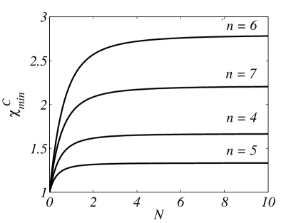
Figure 1: Minimal value of the (dimensionless) cost function $\chi$ versus the (dimensionless) energy constraint parameter $N$, for several values of $n$.

Since it is not possible to find perfect MMESs, it is important to quantify the distribution of entanglement. A good distribution of entanglement should be rather insensitive to a change of bipartition. A fairly distributed multipartite entanglement should therefore be characterized by a distribution (over balanced bipartition) with a small standard deviation FFP . We therefore consider the standard deviation of the purity of the reduced states over balanced bipartitions

$$\Delta\chi:=\sqrt{\left(N+1/2\right)^{2n_{A}}\mathbb{E}\left[\det(\mathbb{V}_{A})^{-1}\right]-\chi^{2}},$$ (56)

with $n_{A}=[n/2]$. We will call a MMES with $\Delta\chi=0$ a uniformly optimal MMES, because it has an optimal distribution of entanglement: entanglement (and frustration) is fairly distributed over all bipartitions that attain the minimal value of purity allowed by frustration. Of course, a perfect MMES is uniformly optimal.

Figure 2 displays the peculiar behavior of the standard deviation of the purity: such standard deviation has a different behavior as a function of $N$ for different values of $n$. For $n=5$ and $6$, MMESs are not perfect. Nonetheless, interestingly enough, they have an optimal distribution of entanglement: $\Delta\chi=0$ (for $n=5,6$). By contrast, a non optimal entanglement distribution has been found for MMES with $n=4$ and $7$. This reminds, mutatis mutandis, of what happens in qubit systems, where frustration appears for $n=4$ and $n\geq 7$ mmes ; Scott ; lit . The numerical analysis shows a $\Delta\chi$ of the non uniformly optimal states which is a concave nondecreasing function of the energy parameter $N$. We notice also in this case the presence of a saturation effect for large values of $N$. These findings are summarized in Table 1.

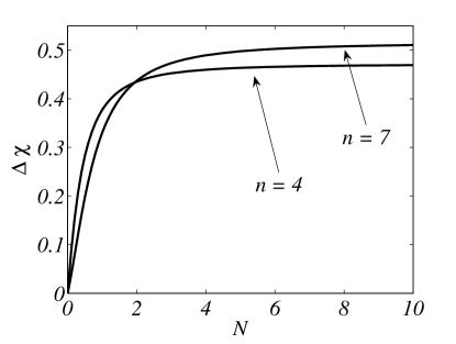
Figure 2: Standard deviation $\Delta\chi$ (dimensionless) of the normalized purity versus the (dimensionless) energy constraint parameter $N$, for $n=4$ and $7$. For $n=5$ and $6$ the MMESs have optimally distributed entanglement, hence vanishing standard deviation.

Table 1: Comparison between qubit and Gaussian maximally multipartite entangled states.

$n$	qubit perfect MMES	Gaussian perfect MMES
2,3	yes	yes
4	no	no
5,6	yes	no, but uniformly optimal∗
7	no∗	no
$\geq 8$	no	no

^∗numerical evidence

VI Conclusions

In conclusion, we have characterized Gaussian states that display a maximal amount of multipartite entanglement compatible with a given constraint on the mean energy. We have shown that perfect Gaussian MMESs (that saturate the maximum mean energy) only exist for $n=2$ and $3$, while the phenomenon of entanglement frustration appears already for $n\geq 4$. Curiously, we found clear numerical evidence that although perfect Gaussian MMESs do not exist for $n=5$ and $6$, for these particular values of $n$, bipartite entanglement can be optimally distributed, in the sense that the standard deviation of purity over balanced bipartitions (56) can be made to vanish. We numerically found that, by contrast, such standard deviation cannot be made to vanish (and bipartite entanglement is therefore not optimally distributed) for $n=4$ and $7$. This peculiar situation is reminiscent of that encountered with qubit MMES, where perfect MMESs exist for $n=5$ and $6$ (qubits), but do not exist for $n=4$ and (probably mmes ) $n=7$. This suggests once more that $n=2,3,5$ and $6$ are “special” integers. We endeavored to summarize these conclusions in Table 1. Experience with integers does not induce us to expect that these amusing peculiarities only occur for $n\leq 6$ (for instance, we numerically found that uniformly optimal MMESs — with vanishing $\Delta\chi$ — exist for $n=9$). Additional research is needed in order to investigate the large $n$ behavior and clarify the underlying structure of entanglement frustration. We emphasize again that this frustration is a consequence of the conflicting requirements that entanglement be maximal for all possible bipartitions of the system. The same phenomenon is also worth studying under different constraints, like, for instance, the (weaker) energy constraint (23).

From a more applicative perspective, we emphasize that due to recent progress in the optical generation of Gaussian entangled states (up to $9$ modes Su ) the above features are also liable to experimental check. These results, combined with those obtained in adesso , and the ensuing proposed characterization of entanglement would help in optimizing multiparty quantum information protocols with continuous variables.

Acknowledgments

The work of PF, GF and SP is partly supported by the EU through the Integrated Project EuroSQIP. The work of CL and SM is supported by EU through the FET-Open Project HIP (FP7-ICT-221899). The authors thank an anonymous referee for an important remark.

References

- (1) V. Vedral, Introduction to Quantum Information Science, Oxford University Press, Oxford (2007).
- (2) E. Schrödinger, Naturwissenschaften 23, 807 (1935).
- (3) A. Einstein, B. Podolsky and N. Rosen, Phys. Rev. 47, 777 (1935).
- (4) S. L. Braunstein and A. K. Pati, Quantum Information with Continuous Variables, Springer, Berlin (2003); N. J. Cerf, G. Leuchs, E. S. Polzik, Quantum Information with Continuous Variables of Atoms and Light, Imperial College Press, London (2007).
- (5) W. K. Wootters, Quantum Inf. Comp. 1, 27 (2001); L. Amico, R. Fazio, A. Osterloh and V. Vedral, Rev. Mod. Phys. 80, 517 (2008); R. Horodecki, P. Horodecki, M. Horodecki and K. Horodecki, Rev. Mod. Phys. 81, 865 (2009); G. Adesso, A. Serafini and F. Illuminati, Open Syst. Inf. Dyn. 12, 189 (2005); B.-G. Englert and K. Wódkiewicz, Phys. Rev. A 65, 054303 (2002).
- (6) P. Facchi, G. Florio, G. Parisi and S. Pascazio, Phys. Rev. A 77, 060304(R) (2008).
- (7) A. J. Scott, Phys. Rev. A 69, 052330 (2004);
- (8) A. Higuchi and A. Sudbery, Phys. Lett. A 273, 213 (2000); I. D. K. Brown, S. Stepney, A. Sudbery and S. L. Braunstein, J. Phys. A 38, 1119 (2005), S. Brierley and A. Higuchi, J. Phys. A 40, 8455 (2007).
- (9) H. J. Kimble, Nature 453, 1023 (2008).
- (10) A. Karlsson and M. Bourennane, Phys. Rev. A 58, 4394 (1998).
- (11) M. Hillery, V. Buzek and A. Berthiaume, Phys. Rev. A 59, 1829 (1999).
- (12) J. Zhang, G. Adesso, C. Xie and K. Peng, Phys. Rev. Lett. 103, 070501 (2009).
- (13) P. Facchi, G. Florio, U. Marzolino, G. Parisi and S. Pascazio J. Phys. A: Math. Theor. 42, 055304 (2009).
- (14) M. M. Wolf, F. Verstraete and J. I. Cirac, Int. J. of Quant. Inf. 1, 465 (2003); M. M. Wolf, F. Verstraete and J. I. Cirac, Phys. Rev. Lett. 92, 087903 (2004); C. M. Dawson and M. A. Nielsen, Phys. Rev. A 69, 052316 (2004).
- (15) R. Simon, N. Mukunda, and B. Dutta, Phys. Rev. A 49, 1567 (1994).
- (16) S. L. Braunstein, P. van Loock, Rev. Mod. Phys. 77, 513 (2005).
- (17) M. de Gosson, Symplectic Geometry and Quantum Mechanics, Birkhauser, Berlin (2006).
- (18) P. Facchi, G. Florio and S. Pascazio, Phys. Rev. A 74, 042331 (2006).
- (19) X. Su, A. Tan, X. Jia, J. Zhang, C. Xie and K. Peng, Phys. Rev. Lett. 98, 070502 (2007); M. Yukawa, R. Ukai, P. van Loock and A. Furusawa, Phys. Rev. A 78, 012301 (2008); T. Aoki, G. Takahashi, T. Kajiya, J. Yoshikawa, S. Braunstein, P. van Loock and A. Furusawa, arXiv:0811.3734.