Coupling different levels of resolution in molecular simulations

Abstract

Simulation schemes that allow to change molecular representation in a subvolume of the simulation box while preserving the equilibrium with the surrounding introduce conceptual problems of thermodynamic consistency. In this work we present a general scheme based on thermodynamic arguments which ensures thermodynamic equilibrium among the molecules of different representation. The robustness of the algorithm is tested for two examples, namely an adaptive resolution simulation, atomistic/coarse-grained, for a liquid of tetrahedral molecules and an adaptive resolution simulation of a binary mixture of tetrahedral molecules and spherical solutes.

I Introduction

In many complex systems, rather small local changes, e.g. of molecular structure due to a mutation or complexation of charged molecular fragments due to the presence of multivalent salt, can have significant consequences for their global properties and function. To understand such phenomena and then derive construction or processing principles from the derived knowledge is one of the key areas of modern basic materials science and related areas. To achieve that goal analytic theory and experiment can only provide limited input. Analytic theory can only deal with highly idealized limiting cases and thus provide rigorous anchor points for any other treatment. On the other hand, experimentally it is most often not possible to provide a detailed microscopic characterization down to the atomistic level in all necessary detail. Because of this numerical modeling is more and more becoming an indispensable tool. The questions described pose central challenges for computational studies. It is in most cases impossible to perform simulations of systems such as a polymer melt, a biological systems of proteins in a membrane or a solution of larger molecules in water on an atomistically detailed level for a long enough time (assuming that atomistic force fields of reliable quality exist). Because of that a variety of multiscale simulation techniques, ranging from straightforward hierarchical parameterizations, see e.g. prllu ; jacs1 ; jacs2 ; karsten1 ; karsten2 ; florianjcp ; vothbook , to interfaced layers of different resolutions see e.g. kax ; Rottler:2002 ; Csanyi:2004 ; Laio:2002 ; Jiang:2004 ; Lu:2005 have been developed. Even if one could perform the all atom simulations mentioned above, the reduction of the huge amount of data to extract an understanding of phenomena and mechanisms already requires a systematic coarse graining. While most techniques are sequential in a way that at a given time the whole system is described with the same representation (level of resolution), in many cases it would be convenient to locally adjust on-the-fly the level of resolution according to the properties of interest, while keeping the larger surrounding on a coarser level. Such an approach would however require full equilibrium between these different regimes.

A typical example is the solvation of a molecule in water where the interesting physics and chemistry occurs within few solvation shells around the molecule while outside the water plays the role of a source of mesoscopic water molecules. Thus one has to interface different molecular models of water (e.g. flexible, rigid, and coarse-grained) and to allow for the exchange of molecules among the different representations. This would properly characterize the relevant physics and chemistry of each region and would properly describe the local fluctuations. The concept above can be generalized in terms of designing an algorithm which interfaces two different force-fields describing the same molecules where the exchange of particles from one region of representation to another (and vice versa) occurs under equilibrium conditions. If this can be done on the basis of a rather general framework, it would allow also to couple rather loosely connected representations, as will be discussed below.

Such force fields may have the same level of resolution (i.e. the molecule carries the same number of degrees of freedom, (DOFs)) or different resolution (for example atomistic and coarse-grained). To the first class of problems belong approaches as those of learn on-the-fly Csanyi:2004 where in a certain region of space the force acting on the atoms is updated on the fly by underlying quantum calculations and is interfaced with a standard classical force-field which describes the interactions in the larger region outside. The number of DOFs may remain the same but the force acting on each atom are different in the different regions. To the second kind of problems belong approaches as those of adaptive resolutions jcp ; pre1 ; annurev ; ensing ; heyden where the molecular models carry different number of DOFs. Extensions to link such particle based approaches to continuum have also successfully been testeddelgado:2008 ; delgado:2009 . So far, a physically consistent theoretically framework which properly describes the change of representation and automatically leads to thermodynamic equilibrium between the different regimes is still missing. Here we study this problem and propose a general framework for such a kind of approaches.

II Adaptive Resolution Concepts

The underlying idea for going from one molecular representation to another is to introduce a transition region at the interface, where the molecules slowly change their representation. In this region they are in equilibrium with their actual surrounding and change continuously until the region of the new representation is reached. There they ”arrive” fully equilibrated within the surrounding described by the new representation. At a first glance a natural way to proceed would be an Energy-based approach where a smooth space dependent function would interpolate between the Hamiltonians corresponding to two force-fields. This approach has been shown to lead to unphysical artifacts inconsistencies pre2 ; jpa ; prelu . To avoid this, we proposed a force based simulation approach called AdResS (Adaptive Resolution Scheme) annurev . Here we extend this with a thermodynamically consistent description of the transition regime, which eventually allows to couple adaptively rather different systems and provides first step to open systems molecular dynamics simulations.

The basic idea is to allow the molecules to experience a smooth transition from one force-field to the other and vice versa without altering the equilibrium of the system. For this we introduce a transition region, where an interpolation function is defined in terms of the position of the center of mass of a molecule. As an example, as applied in the AdResS scheme, for a pair force between molecules $\alpha$ and $\beta$ the formula may be written as:

$${\bf F}_{\alpha\beta}=w(X_{\alpha})w(X_{\beta}){\bf F}_{\alpha\beta}^{A}+[1-w(X_{\alpha})w(X_{\beta})]{\bf F}^{B}_{\alpha\beta}$$ (1)

where ${\bf F}_{\alpha\beta}^{A}$ is the force obtained from the potential of representation $A$ and ${\bf F}_{\alpha\beta}^{B}$ the one obtained from the potential of representation $B$; $w(X)$ is the switching function and depends on the center of mass positions $X_{\alpha}$ and $X_{\beta}$ the two interacting molecules, as indicated in grey in Fig.1.

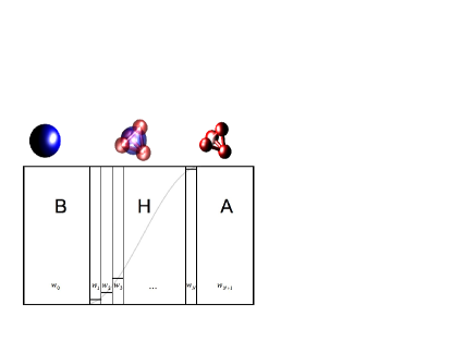
Figure 1: Pictorial representation of the adaptive box and molecular representation. The region on the left, indicated by $B$, is the low resolution (coarse grained) region, the central part is the transition (hybrid) region $H$, where the switching function $w(x)$ (curve in grey) is defined, and the region on the right, indicated by $A$ is the high resolution (atomistic) region. For numerical convenience, as discussed in the text, in order to calculate the chemical potential of each resolution, the transition region is divided in $N$ slides which corresponds to discretized values of the switching function, here indicated with $w_{i}$.

While with the above approach one can perform an MD simulation and control the molecular dynamics, the forces as given in Eq.1 cannot be expressed as the derivative of a Hamiltonian. This rises the question of how to assure the thermodynamic equilibrium in such a force based approach. Indeed our previous studies displayed density fluctuations in the transition regime, which in some cases had to be repaired by a pressure correction term pre1 . The main problem in changing representation in a continuous way is that the DOFs for which the interaction becomes different or which are switched on or off in going from one representation to another are characterized by different energy functions and thus contribute differently to the global equilibrium of the system. This process is associated with the acquisition and release of thermal and interaction energies of these DOFs which must be slowly redistributed as the new representation is acquired. Note that the total energy of the molecules in the different regimes does not at all have to be the same - in most cases it actually will not be the same! These energies related to such a process can be viewed as some sort of latent heat that takes care of the equilibration of the molecules with their environment (see e.g. pre2 ). Switching on and off degrees DOFs can be shown to correspond to fractional DOFs and the related equipartition theorem thus allows to define a temperature and thus a thermostat in the transition regimepre2 ; jpa .

III Generalized Coupling Scheme and Thermodynamic Driving Force

The above intuitive ansatz, can be formalized and generalized within a thermodynamically consistent framework. This theoretical framework allows to explicitly define equations of motion in the transition regime by which both the dynamics and the thermodynamics can be controlled, despite the fact that there is not a well defined energy as in standard simulation schemes. To do this we reformulate the problem in specific terms of an additional thermodynamic force and the internal energy of a molecule as follows.

For the more detailed region $A$ we want to study it as a subsystem at a given temperature $T$ in a fixed volume $V$ with a well defined average number of particles $N$ and pressure $P$. This has to be coupled to a more coarse grained surrounding in a way that the structural and dynamical properties within the region $A$ are (ideally) not altered at all. This also requires that there is no kinetic barrier introduced by the transition regime between $A$ and $B$. Viewing the different regimes as different phases, the question of equilibrium between different regimes generally can be formulated in terms of the differences in the chemical potentialnote2 characterizing each resolution. To do this let us consider the difference $\phi(x)=\mu_{A}-\mu_{w(x)}$ between the chemical potential of a molecule in region $A$ (chemical potential of a system composed solely by high resolution molecules; $w(x)=1$), and in a hybrid system exclusively composed of hybrid molecules with a fixed level of resolution $0\leq w=w(x)=const.\leq 1$ corresponding to a fixed bulk value $\mu_{w(x)}$. Since $w$ in such a hybrid system is constant within the whole system, we now have a well defined energy function, which allows to determine $\mu_{w(x)}$. By repeating this procedure for each value of $x$, we can now approximate an effective, position dependent, chemical potential of the molecules for the whole system, especially in the transition regime in the full range $0\leq w\leq 1$. Since in the adaptive representation scheme $w=w(x)$, $\phi$ becomes a position dependent function in such a simulationnote3 . The wider the transition regime the better this approximation is expected to work, since the difference in the interactions in the direction of growing and shrinking $w$ vanishes. This idea can now be used to couple within one simulation box two systems, where the same molecules are described by different sets of DOFs. Coupling two systems along Eq.1 and running the simulation with a regular Langevin or DPD thermostatannurev ; Junghans often leads to the problem of a nonuniform free energy density throughout the simulation cell, since the free energy density, which to a first approximation depends on the DOFs per molecule, might be different in the different regions. This results then in unwanted density variations especially in the transition regime. As we will see below, the thermostat generally only compensates for part of this problem. In this context $\phi(x)$ is nothing else than the quantity which reintroduces, in an effective way, a formal uniformity.

To calculate $\phi(x)$, we can divide it into two components. The first part is due to the potential of interaction (called ”excess chemical potential”in the following) between the degrees of freedom, which are switched on or off. The second corresponds to the kinetic intramolecular part (internal vibrations and molecular rotations). The latter part typically can also be taken care of by the thermostat (see below). The calculation of the first component can be numerically achieved as illustrated in Fig. 1. The simulation box is divided into a region of force-fields $A$ and $B$ and a transition region $H$ in between. The region $B$ is characterized by the value of the switching function $w_{0}=0$. The region $A$ is characterized by the value of the switching function $w_{N+1}=1$. In $H$ the value of $w$ in the actual simulations varies continuously. However here we approximate this by discretizing $w$ into N steps $w_{1}$, $w_{2}$,… $w_{N-1}$, $w_{N}$. For any fixed value of $w$ the energy function is well defined and the excess chemical potential then is defined as: $\mu^{exc}(x_{i})=\mu^{exc}_{w_{i}}$, where the $\mu^{exc}_{w_{i}}$ is the chemical potential of the molecules in a bulk system of the specific representation of $w_{i}$. To calculate numerically each $\mu^{exc}(w_{i})$ one can use standard particle insertion methods frenkel . Repeating this procedure with all values of $w_{i}$ leads to a position dependent excess chemical potential $\mu^{exc}(x)$. The implicit approximation that each of the stripes in Fig.1 can be taken as a bulk system and is statistically independent of each other will be shown to be of minor importance for practical applications. The second component is the ideal gas kinetic contribution to the chemical potential coming from the internal degrees of freedom. Usually in a “one-representation” simulation, this contribution to the chemical potential is ignored being only a trivial constant. In our case where the DOFs of interest might continuously change in going from one representation to another, each DOF in the transition region contributes differently according to the corresponding value of $w(x)$. While such contributions can be easily calculated for the force-fields $B$ and $A$, the critical aspect to address is what happens for the hybrid representation in the transition region.

For the AdResS scheme we have shown that the interpretation of changing representation as continuous change in dimensionality (between zero and one and vice versa) of the associated phase space of a DOF (see e.g. pre2 ; jpa ; annurev ) allows for a proper definition of the temperature and thus of a thermostat. This means that if a DOF remains unchanged from one representation to another, its dimensionality is one (invariant full contribution to statistical properties regardless of the representation). If instead a DOF is switched on/off from one representation to another its dimensionality goes from one to zero or vice versa; that is if a DOF is explicitly present in force-field $A$ and not present in force-field $B$ it would not contribute to the statistical properties in the region $B$, and would gradually contribute in the transition region up to full contribution in region $A$. In other words the dimensionality of the phase space associated with a DOF reflects the degree of ”representation” expressed by $w(x)$ and it weights, accordingly, its contribution to the average properties of the system. The formalism of fractional calculus has been shown to be able to formally describe this process so that one can calculate the kinetic energy contribution to the free energy per particle jpa . This means that one can calculate the chemical potential for a given representation $w$ analytically and, since $w=w(x)$, obtain the ideal gas contribution. For a generic switchable degree of freedom $p$ this is written as:

$$A_{p}=-\beta\log\left[\int e^{-\beta p^{2}}d^{w}p\right]=\mu^{kin}_{p}(w)$$ (2)

and thus the total contribution of the entire set of switchable degrees of freedom (assuming that they decouple) is:

$$\mu^{kin}(w)=\sum_{DOF}\mu^{kin}_{p}(w).$$ (3)

and the component to the latent heat $\phi(x)^{kin}=\mu^{kin}_{A}-\mu^{kin}(w)$. The solution of Eq.2 can be obtained analytically:

$$\mu^{kin}_{p}(w)=CkT\left(\frac{w}{2}\right)\log(T)+kT\log\frac{\Gamma\left(\frac{w}{2}\right)}{\Gamma\left({w}\right)}$$ (4)

where $C$ is a constant, , $k$ the Boltzmann constant, $T$ is the temperature and $\Gamma$ the standard $\Gamma$ function. The first term in Eq. 4 is linear in $w$ and therefore linearly interpolates between the coarse-grained and all-atom values of $\mu^{kin}$annurev . Note that the second nonlinear term is negligible in the temperature regime of interest. At this point we have a numerical definition of $\mu^{exc}(x)$ and an analytical definition $\mu^{kin}(x)$. In general, the idea of continuous interpolation and the calculation of the latent heat presented here have some formal similarities with the method to calculate entropies or chemical potentials, which can not be calculated directly. This is done by adiabatically coupling via a continuous parameter the real potential to one with a potential where the chemical potential is known and then integrating over that parameter alder . For the pourposes of this work $\mu^{exc}(x)$ $\mu^{kin}(x)$ and are all the ingredients to control the thermodynamic equilibrium of our system and we can use these quantities within the numerical procedure to couple the different resolutions. $\mu^{exc}(x)$ characterizes the chemical potential due to the interactions among molecules according to their representations. Thus the gradient of $\mu^{exc}(x)$ can be interpreted as a thermodynamic force $F_{x}^{TD}=-\frac{\partial\mu^{exc}}{\partial x}$. Subtracted from the standard AdResS forces, Eq.1, should compensate any drift originating from the different resolutions, making the density profile uniform throughout the whole simulation boxnote4 . Similar expressions also emerge in interspecies forces in dense binary systemsZhang . Next, $\mu^{kin}$, is the ”internal” energy of a molecule, independent from the direct interaction with its surroundings, and thus $\phi^{kin}$ it is nothing else than the internal heat that is acquired or removed as the representation changes. Since the temperature is well defined, this can be supplied by any standard local thermostat. One can check a posteriori that indeed this internal heat is in average exactly the amount provided by the thermostat. We have applied the concept described above to two examples, (a) to the adaptive simulation, atomistic/coarse-grained, for a liquid of tetrahedral molecules (see Fig.1 (top)) and (b) to the adaptive simulation of a binary mixture with major component tetrahedral molecules and with spherical solutes (see Fig.5).

IV Applications to model systems

IV.1 (a) Liquid of Tetrahedral Molecules

We first test the above idea on the example of simple tetrahedral molecules, where the molecules can change representation from an atomistic to a coarse-grained resolution and vice versa passing through a series of hybrid representations (see Ref.jcp and Figure 1). This model system also has been used during the first introduction of the AdResS method. In such a system an atomistic representation is interfaced with its corresponding coarse-grained one. We treat the system at temperature $T=\varepsilon/k$ and a liquid density with an atom density of $\rho=0.175/\sigma^{3}\approx 1.0/\sigma_{cg}^{3}$ ($\sigma_{cg}$ is the excluded volume diameter of the coarse-grained molecule). Here $\sigma$ and $\varepsilon$ are the standard Lennard-Jones parameters of length and energy, respectively. For the force field parameters and other modeling details see refs.jcp ; pre1 . The system is set up in such a way, that the equation of state is the same in both the coarse grained and in the all atom regime at the temperature and density of the current simulation. Because of that $\mu^{exc}(x)$ has to be the same for $w=1$ and for $w=0$. As was found in earlier applications of the AdResS algorithm, the coarse grained and the detailed regime are in equilibrium with each other and the molecules are free to move from one regime into the other while simultaneously changing their molecular representation. A typical problem however, as also found in the application of this method to water, were significant density variations within the hybrid regime. Employing the above derived scheme and introducing the corresponding thermodynamic force this problem can be solved. Fig.2 shows $\mu^{exc}$ and the resulting thermodynamic force.

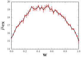
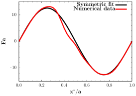
Figure 2: Plot of the excess chemical potential (left) and its thermodynamic force (right). The plot of the force shows, in grey (red) the curve obtained from the numerical data to which a smoothing process was applied and in black the curve obtained from a symmetric fit of the data; both give the same results within the error bar. $a$ is the width of the transition region in reduced units. Because the atomistic and the coarse grained representation describe the same state point they are characterized by the same chemical potential, while this does not hold anymore for the hybrid.

The results of the application of such a force plus the local thermostat for the internal heat is shown in Fig.3 in comparison to the case without that correction.

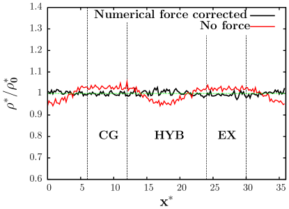
Figure 3: Plot of the density across the simulation box. In grey (red) the case without the thermodynamic force, in black the case where the thermodynamic force is applied. In both cases the system is coupled to a locally acting thermostat. The thermodynamic force clearly improves the quality of the results.

As one can clearly see indeed this procedure leads to a more satisfying density profile which automatically emerges from the forces applied. Remaining very small deviations from the ideally flat profile, which are expected due to the rather approximate way to determine the thermodynamic force, can easily be eliminated in a short iterative procedure, which optimizes the force. In order to prove the full consistency of the method we must still show that the molecular internal heat provided by the thermostat corresponds to that calculated analytically. To do so, we calculate the work done by the thermostat as in Ref.munakata . By removing the contributions of the center of mass we indeed have only the energy corresponding to the internal degrees of freedom.

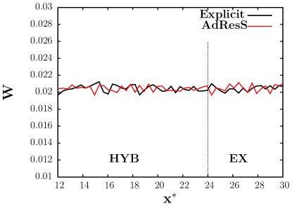
Figure 4: Heat profile provided by the thermostat across the box. The heat is calculated as the work done by the thermostat by removing the contributions of the center of mass. This is the energy corresponding to the internal degrees of freedom.

According to the fractional formalism, the explicit average kinetic energy of a ”switchable” DOF is $w\cdot<K_{atom}>$ pre2 ; jpa . If a thermostat provides an amount of heat $<W_{atom}>$ for the atomistic resolution, it provides an explicit amount of heat $w\cdot<W_{atom}>$ to the hybrid resolutions note . Hence the average extra (latent) heat that the thermostat effectively provides to a molecule in the transition region, in order to have the same internal energy as a molecule in the atomistic resolution, is $<W_{atom}>-w\cdot<W_{atom}>=(1-w)\cdot<W_{atom}>$, that is proportional to the first term in the analytical expression of $\phi^{kin}$. This means that in practice the heat given by the thermostat to the internal DOF’s in the hybrid region is the same as in the atomistic one as consistently obtained in our calculations and shown in Fig.4, while it counts to the total energy of the system only according to the value $w$ in of the actual local resolution. At a first glance the conclusion above seems obvious and can easily be seen for decoupled DOFs. However, the coupling between the intra and the intermolecular interactions is different according to the different resolutions across the box. The equation above provides the first order approximation of heat that must be given by the thermostat according to the formalism introduced in order to have equilibrium across the whole box. In this perspective the numerical calculations indeed indicate that the equation above holds. More important, this proves the robustness of the algorithm regarding the hypothesis of separation between intra and intermolecular DOFs; thus it validates the whole theoretical framework from which the equations governing the switching are obtained. So far, this example shows the validity of the idea of thermodynamic force for a one component system only. However, to apply such an approach to more interesting problems from biophysics or physical chemistry and material science, an extension to the case of multi component systems such as mixtures is needed.

IV.2 Adaptive Resolution Simulation of a Mixture

We now apply the above developed concept to an ”atomistic” liquid of tetrahedral molecules which solvate another species of spherical molecules (see the pictorial representation of the system, Fig. 5).

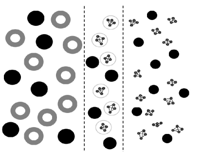
Figure 5: Pictorial representation of the system. On the right the atomistic tetrahedral molecules solvating a spherical solute, in the middle a hybrid representation and on the left the coarse grained one. Notice that the solute, although in all cases one-sited, is characterized by different effective interactions and excluded volume in the different regions since it has to be consistent with the different resolutions of the solvent.

From the atomistic simulation a coarse grained model of both solvent and solute is derived and then the hybrid atomistic/coarse-grained adaptive scheme is applied (for details of the model see note note5 ). Doing this in the conventional wayannurev , leads to significant density variations throughout the system. As for the one component system, we first calculate the chemical potential for each species (solvent and solute) according to the scheme previously shown. However, this is slightly more complex than before, because we have two different molecules each with its intrinsic chemical potential to which the contribution originated by the mixing, both aspects then according to the spatial resolution, must be added. With $c_{i}$ being concentration of component $i$ we can write for the chemical potential of the solvent:

$$\mu^{mix}_{tetra}=\mu^{0}_{tetra}+kT\log[c_{tetra}]+f^{mix}_{int}(c_{tetra},c_{solute})$$ (5)

and equivalently for the solute:

$$\mu^{mix}_{solute}=\mu^{0}_{solute}+kT\log[c_{solute}]+g^{mix}_{int}(c_{tetra},c_{solute})$$ (6)

where $\mu^{0}$ is the chemical potential of the pure component at the same density. $kT\log[c_{i}]$ is the part coming from the entropy of mixing for the ideal noninteracting case for the solvent and solute, respectively. $f^{mix}_{int}(c_{tetra},c_{solute})$ is the part originating from the molecular interactions for the solvent and equivalently $g$ for the solute. The functions $f$ and $g$ are unknown and empirical expressions are given in literature (see e.g. Ref.nieto ; prausnitz ). However, here we have chosen to take a more practical path to determine $f$ and $g$ which can be easily implemented numerically and yet provides the internal consistency the the whole algorithm of simulation. For this we expand $f$ and $g$ as:

$$f^{mix}_{int}(c_{tetra},c_{solute})=\left[\frac{\partial f}{\partial c_{tetra}}\right]_{c_{tetra}^{0},c_{solute}^{0}}\cdot c_{tetra}$$ (7)

$$g^{mix}_{int}(c_{tetra},c_{solute})=\left[\frac{\partial g}{\partial c_{solvent}}\right]_{c_{tetra}^{0},c_{solute}^{0}}\cdot c_{solvent}$$ (8)

here $c_{tetra}^{0},c_{solute}^{0}$ are some equilibrium concentrations which as will be shown are not needed to be known a priori. While all the other quantities entering the chemical potentials are known, the question is how to obtain $\left[\frac{\partial f}{\partial c_{tetra}}\right]_{c_{tetra}^{0},c_{solute}^{0}}$ and $\left[\frac{\partial g}{\partial c_{solvent}}\right]_{c_{tetra}^{0},c_{solute}^{0}}$ as this is needed to obtain the overall thermodynamic force to be applied to each component. To provide a practical approach we first run an adaptive simulation of our system with a thermodynamic force without the terms corresponding to the mixing. Because in the thermodynamic force the terms of the mixing, at this stage, are neglected this simulation will produce a non uniform density profile (or concentration profile) in the transition region. Since we know from Eqs.5,6 and Eqs.7,8 that the terms coming from the mixing are functions of the density (concentration), we take the density profile obtained to determine the terms of mixing, tuning the unknown coefficients of $f$ and $g$ so that the corresponding (complete) thermodynamic force provides a flat profile. By that, we numerically define the unknown part of the chemical potential. As a test of consistency we show that once these constants are fixed, the corresponding thermodynamic force applied to different initial conditions keeps the profile flat and produces a stationary bidirectional flux of particles as for the one component system in Ref.jcp (see Figs.6,7). This is a practical, yet powerful way to determine in general the chemical potential profile of a mixture, consistent with the basic thermodynamical principles of the adaptive representation.

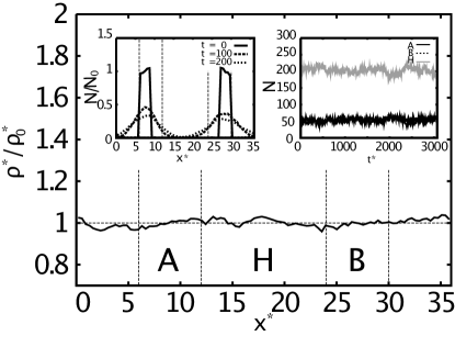
Figure 6: Density profile of the solute across the box. The total number of molecules for the solute is 311, while that of the solvent is 2174, corresponding to a solute concentration of 0.14. Inset, right panel, the total number of molecules in the three regions, as a function of time; $A$ atomistic, $H$ hybrid, $B$ coarse grained. Inset, left panel, diffusion profiles as a function of time of atomistic and coarse grained molecule across the box, the figure display a proper diffusion, assuring that there are no barriers across the system. The three plots show that the system is in a stationary (equilibrium) state. Note that the transition region is larger than the atomistic and the coarse-grained. This was made on purpose because the properties in this region are conceptually of major interest for the development of the current model with the thermodynamic force.

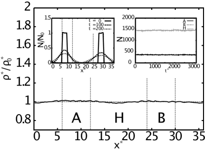
Figure 7: As for Fig.6, now for the solvent.

V Conclusion/Outlook

Our simulation results show how to set up a consistent framework for an adaptive resolution simulation of solutions and mixtures. By the introduction of the concept of a thermodynamic force, based on a locally variable chemical potential, typical artifacts of such a concurrent simulations with variable resolution can be avoided. The method allows for a free exchange of molecules between different regimes and the molecules adapt their very representation according to the region they are in. The approach easily can be extended to more complicated situations, such as systems of even more components. For practical implementations one actually does not have to resort explicitly to the formal derivation via the chemical potential. As illustrated for the case of a mixture, the density profiles in the transition regime can be flattened by a thermodynamic force obtained by a simple numerical tuning. Of course a more formal way to determine the force would end up with the same result. The present approach however is even more general than discussed so far. Usually one deals with a well defined system which one wants to study in different regions of space by different resolutions. This allows to zoom in within a molecular simulation and to study regions of special interest in more detail. The present ansatz on the other hand can be extended to a much wider class of problems. There is absolutely no reason to restrict the method to the case of $\mu=0$ in the pure atomistic and coarse grained region. In principle on can by such a method couple systems with (almost) arbitrary differences and keeps them in equilibrium with each other. Though this might look a bit unexpected, this allows for instance to introduce concepts of open systems or grand canonical molecular dynamics simulations. This will also be of special interest when it comes to non-equilibrium situations like the change of concentrations of one species in the surrounding etc.

- (1) Delle Site L, Abrams C F, Alavi A, Kremer K (2002) Polymers near metal surfaces: Selective adsorption and global conformations. Phys Rev Lett 89: 156103.
- (2) Delle Site L, Leon S, Kremer K (2004) BPA-PC on a Ni(111) surface: The interplay between adsorption energy and conformational entropy for different chain-end modifications. J Am Chem Soc 126: 2944-2955.
- (3) Ghiringhelli L, Hess B, van der Vegt N F A, Delle Site L (2008) Competing adsorption between hydrated peptides and water onto metal surfaces: From electronic to conformational properties. Am Chem Soc 130: 13460-13464.
- (4) Reuter K, Frenkel D, Scheffler M (2004) The steady state of heterogeneous catalysis, studied by first-principles statistical mechanics. Phys Rev Lett 93: 116105.
- (5) Rogal J, Reuter K, Scheffler M (2008) CO oxidation on Pd(100) at technologically relevant pressure conditions: First-principles kinetic Monte Carlo study. Phys Rev B 77: 155410.
- (6) Tarmyshov K, Müller-Plathe F (2007) Interface between platinum(111) and liquid isopropanol(2-propanol): A model for molecular dynamics studies. J Chem Phys 126: 074702.
- (7) in Coarse-Graining of Condensed Phase and Biomolecular Systems, ed Voth G A (Chapman and Hall/CRC Press, Taylor and Francis Group). (2008)
- (8) Lu G, Tadmor E B, Kaxiras E (2006) From electrons to finite elements: A concurrent multiscale approach for metals. Phys Rev B 73: 024108.
- (9) Rottler J, Barsky S, Robbins M O (2002) Cracks and crazes: On calculating the macroscopic fracture energy of glassy polymers from molecular simulations. Phys Rev Lett 89: 148304.
- (10) Csanyi G, Albaret T, Payne M C, Vita A D (2004) “Learn on the fly”: A hybrid classical and quantum-mechanical molecular dynamics simulation. Phys Rev Lett 93: 175503.
- (11) Laio A, VandeVondele J, Röthlisberger U (2002) A Hamiltonian electrostatic coupling scheme for hybrid Car-Parrinello molecular dynamics simulations. J Chem Phys 116: 6941-6947.
- (12) Jiang D E, Carter E A (2004) First principles assessment of ideal fracture energies of materials with mobile impurities: implications for hydrogen embrittlement of metals. Acta Mater 52: 4801-4807.
- (13) Lu G, Kaxiras E (2005) Hydrogen embrittlement of aluminium: The crucial role of vacancies. Phys Rev Lett 94: 155501.
- (14) Praprotnik M, Delle Site L, Kremer K (2005) Adaptive resolution molecular-dynamics simulation: Changing the degrees of freedom on the fly. J Chem Phys 123: 224106.
- (15) Praprotnik M, Delle Site L, Kremer K (2006) Adaptive resolution scheme for efficient hybrid atomistic-mesoscale molecular dynamics simulations of dense liquids. Phys Rev E 73: 066701.
- (16) Praprotnik M, Delle Site L, Kremer K (2008) Multiscale simulation of soft matter: From scale bridging to adaptive resolution. Annu Rev Phys Chem 59: 545-571.
- (17) Ensing B, Nielsen S O, Moore P B, Klein M L, Parrinello M (2007) Energy conservation in adaptive hybrid atomistic/coarse-grain molecular dynamics. J Chem Theory Comput 3: 1100-1105.
- (18) Heyden A, Truhlar D G (2008) Conservative algorithm for an adaptive change of resolution in mixed atomistic/coarse-grained multiscale simulations. J Chem Theory Comput 4: 217-221.
- (19) Delgado-Buscalioni R, Kremer K, Praprotnik M (2008) Concurrent triple-scale simulation of molecular liquids. J Chem Phys 128: 114110.
- (20) Delgado-Buscalioni R, Kremer K, Praprotnik M (2009) submitted.
- (21) Praprotnik M, Kremer K, Delle Site L (2007) Adaptive molecular resolution via a continuous change of the phase space dimensionality. Phys Rev E 75: 017701.
- (22) Praprotnik M, Kremer K, Delle Site L (2007) Fractional dimensions of phase space variables: a tool for varying the degrees of freedom of a system in a multiscale treatment. J Phys A: Math Gen 40: F281-F288.
- (23) Delle Site L (2007) Some fundamental problems for an energy-conserving adaptive-resolution molecular dynamics scheme. Phys Rev E 76: 047701.
- (24) Alternatively, one also could use the pressures and, for mixtures, partial pressures for a similar scheme. Because pressure only requires forces, it is well defined within the whole simulation box. We here however use the chemical potentials, since this allows us more easily to formulate the setup in a more general way.
- (25) In practice, this is exact only for a vanishing slope of , since in the actual simulation in the hybrid regime the molecules interact with other molecules of slightly different representation. This however, as will be seen below, is a rather good approximation.
- (26) Junghans C, Praprotnik M, Kremer K (2008) Transport properties controlled by a thermostat: An extended dissipative particle dynamics thermostat. Soft Matter 4: 156.
- (27) Frenkel D, Smit B (1996) in Understanding Molecular Simulation: From Algorithms to Applications (Academic Press, San Diego), pp 172-176.
- (28) Kirkwood JG, Maun EK, Alder BJ (1950) Radial distribution functions and the equation of state of a fluid composed of rigid spherical molecules. J Chem Phys 18: 1040.
- (29) Actually, this method could also be used to introduce a density gradient on purpose and thus to couple rather different systems.
- (30) Zhang D Z, Ma X, Rauenzahn R M (2006) Interspecies stress in momentum equations for dense binary particulate systems. Phys Rev Lett 97: 048301.
- (31) Munakata T (1999) Mechanical and Langevin thermostats: Gulton staircase problem. Phys Rev E 59: 5045.
- (32) The kinetic energy of a given hybrid molecule can be written asjpa : , where is the kinetic energy of the coarse-grained molecule, is the intramolecular kinetic energy corresponding to molecular rotational and vibrational DOFs (these DOFs are switched on/off while changing the resolution), is the kinetic energy associated with the fractal rotational+vibrational DOFs that are explicitely considered in the simulation, is the total internal kinetic energy associated with those fractal DOFs that are not explicitely considered in our treatment, and is the degree of fractionality (the degree of how much a particular DOF is switched on). During the adaptive resolution simulation the explicit DOFs of the hybrid molecules, i.e., rotational + vibrational DOFs, are also equilibrated. The explicit DOFs of a given hybrid molecule are fully present in the simulation regardless of the hybrid molecules’ position in the transition regime but they contribute differently to the statistical averages (depending on ). The switching on/off DOFs has to be understood in the statistical sense, i.e., how much of a particular DOF contribution is explicitly considered in the statistical-mechanical averages. Therefore, the thermostat has to supply or remove the same amount of kinetic energy to/from the explicit DOFs of the hybrid molecules in the transition regime as it does in the case of the fully explicit molecules in the all-atom regime in order to keep the system at given temperature. The part of this energy contributes to the while the part is ascribed to . The latter represents a part of the latent heat associated with the change of the resolution.
- (33) We have developed the coarse-grained potentials that reproduce the thermodynamic state point and basic structure of two atomistic mixtures: one, at densities of 0.174 for the solvent and 0.001 for the solute, in Lennard-Jones reduced units, and a more concentrated system with densities of 0.151 and 0.022 respectively. In both cases the pressure matches the value obtained from the pure tetrahedral liquid previously studied. The interactions were parameterized using the Iterative Boltzmann method as in Ref.jcp . By these means, we obtained a first guess for the coarse-grained potential between the two species for the most diluted mixture. Next we proceeded to reparametrize the solvent-solvent interaction on the most concentrated system and further tune the potential between both species to conclude with the refinement of the force field between the solute particles until the radial distribution functions between solvent, solute and both kinds of particles are in good agreement with the atomistic simulations. In addition, the set of potentials obtained in this way reproduces accurately the pressure for the highest concentration and below
- (34) Nieto R, Gonzales M C, Herrero F (1999) Thermodynamics of mixtures: Functions of mixing and excess functions. Am J Phys 67: 1096-1099.
- (35) Prausnitz J M, Lichtenthaler R N, Gomes de Acevedo E (1999) in Molecular Thermodynamics of Fluid-Phase Equilibria, (Patience Hall PTR, Upper Saddle River, New Jersey), pp 214-299.