Extensive analytical and numerical investigation of the kinetic and stochastic Cantor set

Abstract

We investigate, both analytically and numerically, the kinetic and stochastic counterpart of the triadic Cantor set. The generator that divides an interval either into three equal pieces or into three pieces randomly and remove the middle third is applied to only one interval, picked with probability proportional to its size, at each generation step in the kinetic and stochastic Cantor set respectively. We show that the fractal dimension of the kinetic Cantor set coincides with that of its classical counterpart despite the apparent differences in the spatial distribution of the intervals. For the stochastic Cantor set, however, we find that the resulting set has fractal dimension $d_{f}=0.56155$ which is less than its classical value $d_{f}={{\ln 2}\over{\ln 3}}$. Nonetheless, in all three cases we show that the sum of the $d_{f}$th power, $d_{f}$ being the fractal dimension of the respective set, of all the intervals at all time is equal to one or the size of the initiator $[0,1]$ regardless of whether it is recursive, kinetic or stochastic Cantor set. Besides, we propose exact algorithms for both the variants which can capture the complete dynamics described by the rate equation used to solve the respective model analytically. The perfect agreement between our analytical and numerical simulation is a clear testament to that.

I Introduction

The history of describing natural objects by geometry is as old as the history of science itself. Perhaps, the oldest of our pedagogical understanding about the properties of physical objects is geometry. Thanks to the Greek philosopher Euclid who is in fact the principal architect for laying the early foundation of geometry which is now known as the Euclidean geometry. For centuries, it has been the only means of describing geometry of physical objects. However, the then scientists also realized that the nature is not restricted to Euclidean space only; instead, most of the natural objects we see around us are so complex in shape that conventional Euclidean space is not sufficient to describe them. It was not until the work of Benoit B. Mandelbrot that dramatic progress was made. In 1975 Mandelbrot introduced the idea of fractal that has revolutionized the whole concept of geometry ref.mandelbrot1 . Prior to the inception of fractal, geometry remained one of the main branches of mathematics. However, soon after its inception, it has attracted mathematicians, physicists, and engineers all alike and hence generated a widespread interest. All credit goes to Mandelbrot for the way he presented the idea of fractal through his monumental book The Fractal Geometry of nature ref.mandelbrot2 . Indeed, he presented his book in an unusually inspiring way and since then it remained as the most favourite standard reference book for both beginners and researchers. Due to its wide interest, it has brought many seemingly unrelated subjects under one umbrella and provided a tools to appreciate that there exists some kind of order even in the seemingly complex and apparently disordered many natural geometric structures.

The importance of fractal and multifractal in nonlinear dynamics especially in chaos can hardly be exaggerated. Their relation exist to such an extent that the impact of the ideas of chaos and fractals in physics and other scientific disciplines in recent years have been enormous. One common thing about both chaos and fractals is that much of their progress was possible due to high configuration computers and numerical simulations. Interestingly, the real progress of fractals and chaos both began during the 1970s. Most of the books or articles written on chaos are found to invoke the idea of fractal since the plot of the fractal basins associated with chaos provides a qualitative idea of the extent of complications in the prediction of its future evolution ref.rmp . For this and because of their common history often general people regards the two concepts synonymous. Note that the keywords in chaos are non-linearity, unpredictability, sensitivity to initial conditions. On the other hand, the keywords in fractals are self-similarity and scale-invariance that is, the objects look the same on different scales of observation.

The exact definition of fractal even after all these years is still elusive. Mandelbrot himself was somehow reluctant to confine it within the boundaries of a mere definition. He, nevertheless proposed that fractal can be defined as a geometric object which is similar to itself on all scales. That is, if one zooms in on a fractal object it will look exactly similar to the original shape. Mandelbrot offered also a mathematical definition ”a fractal is by definition a set for which the Hausdorff-Besicovitch dimension strictly exceeds the topological dimension”. Sometimes fractal is also defined in terms of mass-length relation ref.vicsek . That is, if the mass $M$ of an object is related to its different possible size $L$ by the relation

$$M(L)\sim L^{d_{f}},$$ (1)

where $d_{f}$ is less than the dimension of the space in which the object is embedded then the object is called fractal and it is quantified by its dimension $d_{f}$.

The Hausdorff-Besicovitch dimension actually plays the pivotal role for a rigorous definition of fractal and for providing a procedure to find the fractal dimension. Consider that the measure $M_{d}$ is the size of the set of points in space of the object. We can quantify the size of the measure $M_{d}$ by using $d$-dimensional hypercube of linear size $\delta$ as a yardstick to find the number $N(\delta)$ needed to cover $M_{d}$ ref.feder . That is, we can cover the object to form the measure

$$M_{d}=\sum\delta^{d}=N(\delta)\delta^{d},$$ (2)

where $\delta^{d}$ is the test function. The number $N(\delta)$ will obviously gets smaller as the size of the yardtick $\delta$ gets larger. It can be easily shown that $N(\delta)$ satisfies the following generalized relation

$$N(\delta/n)=n^{d_{E}}N(\delta),$$ (3)

if $M_{d}$ describes an Euclidean object. The above relation for $N$ satisfies the property of a homogeneous function $N(\lambda x)=\lambda^{p}N(x)$ if one chooses $\lambda=n^{-1}$, $x=\delta$ and $p=-d_{E}$. One can explicitly prove that only power-law solution can satisfy Eq. (3) ref.newman . Indeed, it is easy to check that $N(\delta)\sim\delta^{-d_{E}}$ can solve Eq. (3). In reality there exist another class of objects which also exhibits a similar power-law relation between the number $N$ and the size of the yardstick $\delta$ but with a non-integer exponent $d_{f}$ instead of $d_{E}$ and hence one can generalize the relation as

$$N(\delta)\sim\delta^{-D},$$ (4)

where $D$ is called the Hausdorff-Besicovitch (H-B) dimension ref.feder . Using this relation in Eq. (2) we find that the value of $M_{d}$ assumes a finite constant value only if $d=D$ otherwise the measure $M_{d}$ is either zero if $d>D$ or infinity if $d<D$ in the limit $\delta\rightarrow 0$. The H-B dimension therefore is the critical dimension $d=D$ for which the measure $M_{d}$ neither vanishes nor diverges as $\delta\rightarrow 0$. So, an object is fractal if the H-B dimension $D=d_{f}$ a non-integer value.

The best known text example of fractal is the triadic Cantor set. However, this classical Cantor set lacks in two ways from the natural fractals. Firstly, it does not appear through evolution in time although fractals in nature do so. Secondly, it is not governed by any sort of randomness throughout its construction. On the other hand, natural fractals always occur through some kind of evolution accompanied by some randomness. In this article, we therefore, investigate two interesting variants of the classical Cantor set, the kinetic and the stochastic Cantor set, in which time and randomness are incorporated in a logical progression. The kinetic Cantor set differs from the classical Cantor set in the sense that at each step only one of the available interval is picked, with probability proportional to its size, for dividing it into three equal pieces and remove the middle third. On the other hand, in the stochastic Cantor set the definition of the generator is modified in the sense that it divides an interval into three pieces randomly and remove the middle third. However, the modified generator is applied sequentially to only one interval which is also picked according to its size at each generation step like in the kinetic Cantor set. The adventage of applying the generator sequentially is that we can invoke time as one of the parameter in the problem. On the other hand modifying the generator in the stochastic Cantor set incorporate randomness into the problem as it evolves. In fact, it is well understood that in our world almost nothing is stationary or strictly deterministic. Every natural objects are seemingly complex in character though they are governed by simple rules since simple rules when repeated over and over again can appear mighty complex.

The Cantor set provides us with a wealth of interesting properties which are taught in advanced undergraduate and graduate studies in discrete mathematics course. Apart from its pedagogical importance the Cantor set problem has also been of theoretical and practical interest. For instance, Sears et al has shown that a nonlinear system that supports solitons can be driven to generate Cantor set ref.sears . In another case, it has been found that the electromagnetic wave is strongly enhanced and localized in the cavity of the Cantor set near the resonant frequency ref.hatano . Krapivsky and Redner shown that the probability distribution in a random walk with a shrinking steps is a Cantor set ref.redner . Recently, Esaki et al studied propagation of waves through Cantor set media and found some very interesting results such as complete reflection or complete transmission including scaling property of the transmission co-efficients ref.esaki .

The remainder of this article is organized as follows. In section II, titled ’recursive Cantor set’ we discussed the well-known triadic Cantor set. In section III, we proposed the kinetic counterpart of the triadic Cantor set and solved it exactly to obtain the fractal dimension and various other properties. We also proposed exact algorithm for the kinetic Cantor set to solve the model by numerical simulation. In section IV, we investigated the stochastic counterpart of the triadic Cantor set and once again we proposed its exact algorithm to solve it by numerical simulation. In section V, we summarized our results.

II Recursive Cantor set (RCS)

The novelty in the definition of the triadic Cantor set is its simplicity. The notion of fractal and its inherent character, self-similarity, is almost always introduced to the beginner through this example. The triadic Cantor set can be defined as follows. It starts with an initiator of unit interval $[0,1]$. The generator then divides it into three equal parts and deletes the middle third leaving behind two sub-intervals, each with size one-third of the original interval such as $[0,{{1}\over{3}}]$ and $[{{2}\over{3}},1]$. In the next step, the generator is again applied to each of the two sub-intervals that divides them into three equal parts of size ${{1}\over{9}}$ and remove the middle third from both. The process is then continued by applying the generator on the remaining intervals recursively ad infinitum and hence we call it recursive Cantor set (RCS). Like its definition, finding the fractal dimension of the RCS problem is also trivially simple. According to the construction of the RCS process there are $N=2^{n}$ intervals in the $n$th generation each of size $\delta=3^{-n}$ and hence it is also the mean interval size. The most convenient yard-stick in the $n$th step, therefore, is the mean interval size $\delta=3^{-n}$. The generation number $n$ can be written as

$$n=-{{\ln\delta}\over{\ln 3}}.$$ (5)

Using it in $N=2^{n}$ we find that the number $N$ falls off following power-law against mean interval size $\delta$ i.e.,

$$N(\delta)\sim\delta^{-d_{f}},$$ (6)

with $d_{f}={{\ln 2}\over{\ln 3}}$. Since the exponent $d_{f}$ of the above relation is non-integer and at the same time it is less than the dimension of the space $d=1$ where the set is embedded, it is the fractal dimension of the resulting triadic Cantor set. Note that the set does not fill up the unit interval by uniform distribution of zero-dimensional points to describe a line rather, it fills up the unit interval by zero-dimensional points (also known as the Cantor dust) in such a special way that it possess exact self-similarity.

III Kinetic Cantor set (KCS)

One may wonder what if we divide only one interval at each step instead of dividing every available intervals as done in the RCS problem? Clearly, the spatial distribution of intervals along the line will be very different from the one created by the RCS problem. But, then the question is: Will the number $N$ needed to cover the set by an yardstick, say of size $\delta$, still exhibit power-law against $\delta$? If yes, will the exponent vis-a-vis the fractal dimension be the same as for the RCS? To find a definite answer to these questions, the same generator that divides an interval into three equal pieces and remove the middle third in the RCS problem is applied to only one of the available intervals instead of applying it to each of the available intervals at each step. But after step one and beyond the system will have intervals of different sizes and hence it raises further question: How do we choose one interval when the system has more than one interval of different sizes? We choose the case whereby an interval is picked with probability proportional to their respective sizes as it appears to be the most generic case. One advantage of modifying the RCS problem in this way is that we can use the rate equation approach to solve it analytically. Since time becomes one parameter of the problem we call it kinetic Cantor set (KCS).

The KCS problem can be defined as follows. Like RCS it may also starts with an initiator of unit interval $[0,1]$. In the first step the generator therefore divides the initiator into three sub-intervals of equal size and remove the middle third. The two newly created intervals are labelled as $1$ and $2$ starting from the left end of the two surviving intervals. In the next step we generate a random number $R$ from the open interval $(0,1)$ and find which of the two subintervals $1$ and $2$ contains this number $R$ in order to ensure that intervals are picked according to their size. If $R$ is found within the interval $[0,{{1}\over{3}}]$ then we pick interval $1$, if it is found within $[{{2}\over{3}},1]$ we pick interval $2$. Say, the interval $1$ contain $R$ and hence we pick interval $1$. The generator then divides it into three equal pieces and remove the middle third. The left end of the two newly created interval is then labelled with its parent label $1$ and the intervals on its right is labelled as $3$. In any case, time is increased by one unit even if $R$ is found within the interval that has been removed. Note that between two successive generation steps the time unit may increase by several units since each time an attempt in picking an interval is unsuccessful the time is increased by one unit. One therefore cannot write a straightforward relation between time $t$ and generation step $j$ although we will explore later that there do exist a non-trivial relation between $N=(j+1)$ and time $t$. The $j$th step therefore starts with $j$ number of intervals labelled as $1,2,...,j$ and at the end of the $j$th step the system will have $j+1$ intervals whose sizes can be denoted as $x_{1},x_{2},...,x_{j+1}$. The basic algorithm of the $j$th step which starts with $j$ number of intervals can be described as follows.

• Generate a random number $R$ from the open interval $(0,1)$.

• Check which of the $1,2,...,j$ intervals contains the random number $R$. Say, the interval that contain $R$ is labelled as $m$ and hence pick the interval $m$. Else, if none of the $j$ intervals contain $R$ then increase time by one unit and go to step $(a)$.

• Apply the generator to the sub-interval $m$ to divide it into three equal pieces and remove the middle third.

• Label two newly created intervals starting from the left end which is labelled with its parents label $m$ and the interval on the right is labelled with a new number $j+1$ that has not been already used.

• Increase time by one unit.

• Repeat the steps $(a)$-$(e)$ ad infinitum.

The expression for the mean interval size after the $j$th step therefore is $\delta=\sum_{i}^{j+1}x_{i}/(j+1)$ and the corresponding time $t$ can be obtained from the counter used for time in the algorithm.

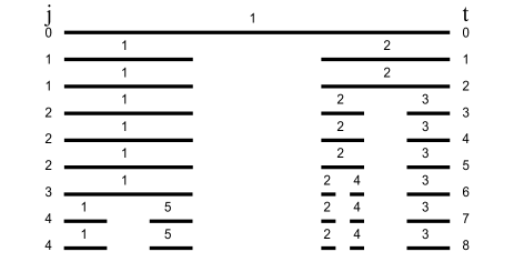
Figure 1: Schematic illustration of the construction of the kinetic Cantor set. On the left the numbers below $j$ indicates generation steps which is related to number of intervals via $N=j+1$. On the right the numbers below $t$ indicates increase in time which is related to $N$ via a non-trivial relation that we will explore.

To solve the KCS problem analytically we use the rate equation approach. The state of the system at any time $t$ can be characterized fully by the interval size distribution function $C(x,t)$ which is defined in such a way that $C(x,t)dx$ is the number of intervals in the size range $x$ and $x+dx$ at time $t$. The evolution of the distribution function $C(x,t)$ can then be described by the following master equation

$${{\partial C(x,t)}\over{\partial t}} = -C(x,t)\int_{0}^{x}dy\int_{0}^{x-y}F(y,z|x)dz$$ (7)

$$+ 2\int_{x}^{\infty}dyC(y,t)\int_{0}^{y-x}F(x,z|y)dz,$$

where the kernel $F(x,y|z)$ describes the rate and rules how a parent interval of size $z$ is divided into three smaller intervals of size $x$, $y$ and $(z-x-y)$. The first term on the right hand side of the above rate equation describes the loss of interval of size $x$ due to breakup of an interval of size $x$ while the second term describes the gain of interval of size $x$ due to breakup of an interval of size $y>x$ into three smaller pieces so that at least one of the three smaller intervals is of size $x$. The factor $2$ in the gain term guarantees that only two of the three intervals are kept and one is removed which is exactly the definition of the Cantor set. Note that if the factor $2$ in Eq. (7) is replaced by the factor $3$, then the resulting equation describes the kinetics of ternary fragmentation process. The ternary fragmentation equation was first proposed and solved exactly by Ziff ref.ziff . In order to mimic the generator that picks an intervals according to size of the available intervals and divide it into three equal pieces we choose

$$F(x,y|x+y+z)=(x+y+z)\delta(x-y)\delta(y-z).$$ (8)

where the two delta functions ensures that the three intervals produced by the generator are equal in size. Substituting this kernel into Eq. (7) we get

$${{\partial C(x,t)}\over{\partial t}}=-{{x}\over{3}}C(x,t)+6xC(3x,t).$$ (9)

One can solve the above equation exactly to find the solution for $C(x,t)$ using the Laplace transformation.

We are not really interested in the solution for the distribution function $C(x,t)$ rather we are interested in finding solution of its $n$th moment defined as

$$M_{n}(t)=\int_{0}^{\infty}x^{n}C(x,t)dx,$$ (10)

as it can provide almost all the information that we intend to find. Moreover, we find it more convenient to analyze the moment of the distribution function than the function itself. Incorporating the definition of the $n$th moment in Eq. (9) yield the following rate equation for the $n$th moment

$${{M_{n}(t)}\over{dt}}=\Big{[}{{1}\over{3}}-{{2}\over{3^{n+1}}}\Big{]}M_{n+1}(t).$$ (11)

It is interesting to note that the distribution function $C(x,t)$ is not a directly observable quantity but its various moments are, for instance, $M_{0}(t)=N(t)$ is the number of available intervals at time $t$, $M_{1}(t)=L$ is the sum of the sizes of all the available intervals at time $t$ etc. This clearly justifies the reason behind focusing on finding the solution for the various moments than the distribution function itself. For consistency check, let us consider a case whereby none of intervals are removed after generator divides an interval into three equal pieces. That is, the sum of the sizes of all the intervals at all time would be equal to the size of the initiator. The corresponding rate equation for $M_{n}(t)$ which can be obtained from Eq. (11) upon replacing the factor $2$ by $3$ from which one can easily find that

$${{dM_{1}}\over{dt}}=0,$$ (12)

and hence $M_{1}(t)=L$ is indeed independent of time which is infact equal to the size of the initiator.

In order to obtain a complete solution for the $n$th moment of Eq. (11) we assume that there exists a value $n=n^{*}$ so that $M_{n^{*}}$ remains independent of time or a conserved quantity in the long time limit. Indeed, a closer look into the rate equation for the $n$th moment immediately implies that we can obtain the value of $n^{*}$ by applying the steady-state condition

$$\lim_{t\longrightarrow\infty}{{dM_{n}(t)}\over{dt}}=0,$$ (13)

in Eq. (11) and hence obtain the following equation

$${{1}\over{3}}-{{2}\over{3^{n^{*}+1}}}=0.$$ (14)

Solving it for $n^{*}$ we immediately find that $n^{*}={{\ln 2}\over{\ln 3}}$ which implies that $M_{{{\ln 2}\over{\ln 3}}}$ is a conserved quantity. One of the property of fractal is that it must obey scaling or self-similarity. As we are expecting that the KCS problem like its cousin RCS problem will also generate fractal in the long time limit. It is therefore reasonable to anticipate that the solution of Eq. (9) for general $n$ will exhibit scaling. Existence of scaling means that the various moments of $C(x,t)$ should have power-law relation with time and hence we can write a tentative solution of Eq. (11) as below

$$M_{n}(t)\sim A(n)t^{\alpha(n)}.$$ (15)

If we insist that it must obey the conservation law, $M_{{{\ln 2}\over{\ln 3}}}=const.$ then we must have $\alpha(\ln 2/\ln 3)=0$. Substituting this in Eq. (11) we obtain the following recursion relation

$$\alpha(n+1)=\alpha(n)-1.$$ (16)

Iterating it subject to the condition that $\alpha(\ln 2/\ln 3)=0$ gives

$$\alpha(n)=-(n-{{\ln 2}\over{\ln 3}}).$$ (17)

We therefore now have an explicit asymptotic solution for the $n$th moment

$$M_{n}(t)\sim t^{\Big{(}n-{{\ln 2}\over{\ln 3}}\Big{)}Z},\hskip 9.95863pt{\rm where}\hskip 9.95863ptZ=-1.$$ (18)

According to Eq. (18) we find that the number of intervals $N(t)=M_{0}(t)$ grows as

$$N(t)\sim t^{{{\ln 2}\over{\ln 3}}},$$ (19)

and the mass or the sum of all the intervals size decreases against time as

$$M(t)\sim t^{-0.369}.$$ (20)

The solutions for $M_{0}(t)$ and $M_{1}(t)$ can provide us with the information how the mean interval size $\delta(t)=M_{1}(t)/M_{0}(t)$ decay and find that

$$\delta\sim t^{Z},$$ (21)

where the kinetic exponent $Z=-1$. We now apply the idea of fractal analysis which is briefly described in the introduction. To this end we find it convenient to use typical or mean interval size $\delta(t)$ as the yard-stick to measure the resulting set since it will always give an integer $N$. This is equivalent to expressing the number $N$ in terms of $\delta$ and in doing so we find that $N(\delta)$ decreases following the same power-law as Eq. (6) including its exponent $d_{f}={{\ln 2}\over{\ln 3}}$. The H-B dimension of the resulting KCS problem therefore is $D={{\ln 2}\over{\ln 3}}$ which is exactly the same as its recursive counterpart albeit the spatial distribution is very different.

Figure 2: The decrease in mean interval size $\delta$ against time $t$, as defined in the algorithm, is drawn in the $\log-\log$ scale using numerical data and found that it satisfies $\delta\sim t^{-1}$ which is also predicted by analytical solution.

Figure 3: Plots of $\log(N)$ vs $\log(\delta)$ is drawn using numerical data. The line has slope equal to $d_{f}={{\ln 2}\over{\ln 3}}$ revealing $N\sim\delta^{-d_{f}}$ as predicted by the theory.

Figure 4: The sum of the $d_{f}$th power of all the intervals $x_{1}^{d_{f}}+x_{2}^{d_{f}}+...+x_{j}^{d_{f}}=1$ regardless of time if $d_{f}={{\ln 2}\over{\ln 3}}$ which is equal to fractal dimension of the kinetic Cantor set. Its analytical counterpart is the $d_{f}$th moment of the distribution function.

To verify our analytical results we performed Monte Carlo simulation based on the algorithm (a)-(f). We first collected data for the mean intervals size $\delta=\sum_{i}^{j+1}x_{i}/(j+1)$ against time where $x_{i}$s are the size of the intervals specified by their labels $i=1,2,....,j$. This data is used to draw $\log(\delta)$ vs $\log(t)$ in Fig. (2) and we clearly find a straight line with slope equal to $1$ revealing that the mean interval size decreases following the same inverse power-law as predicted by Eq. (21). Numerical data are also used to plot $\log(N)$ against $\log(\delta)$ and again we find a straight line but with a slope equal to ${{\ln 2}\over{\ln 3}}$ which is exactly as predicted by our theory (see Fig. (3)). It clearly proves that the underlying mechanism described by the Eq. (9) has been captured by the algorithm (a)-(f) we proposed for the KCS problem. One may think of another variant of the kinetic Cantor set by removing one of the three intervals randomly each time generator divides an interval into three equal intervals. Surprisingly, numerical data reveals that the value of $d_{f}$ still is the same regardless of exactly which of the three intervals is removed each time an interval is divided into three equal intervals. Indeed, the rate equation for the distribution function $C(x,t)$ given by Eq. (9) do not distinguish the three smaller intervals from one another. Now, incorporating $d_{f}={{\ln 2}\over{\ln 3}}$ in Eq. (18) we can conclude that the moment of order equal to fractal dimension $d_{f}$ is a conserved quantity. To verify this we collected data for the sum of the $d_{f}$th power of the size of all the intervals available at the generation step $j$ and found

$$x_{1}^{d_{f}}+x_{2}^{d_{f}}+x_{3}^{d_{f}}+...\ ...\ +x_{j}^{d_{f}}=1,$$ (22)

regardless of the value of $j$ vis-a-vis time $t$ which is equivalent to $M_{d_{f}}$. This is quite an extra-ordinary revelation. This result make us wonder if such conservation law also exist in the case of traditional recursive Cantor set. Due to recursive nature of the RCS problem, after any generation step $n$ all the $N=2^{n}$ intervals will have the same size $3^{-n}$. The sum of the $d_{f}$th power of all the intervals after the $n$th generation step therefore is

$$2^{n}\Big{(}3^{-n}\Big{)}^{{{\ln 2}\over{\ln 3}}}=1,$$ (23)

regardless of the value of $n$. We wonder what if we further modify the generator to create the stochastic fractal instead of random fractal. Will the relation that the sum of the $d_{f}$th power of all the intervals at any given time be the same with that of at any other time?

IV Stochastic Cantor set (SCS)

The RCS problem hardly has any relevance to the fractal that appear in nature as it lacks at least in two ways from those that occur in nature. For instance, it does not have any kinetics but most natural fractal appears through some kind of evolution and it does not have any randomness but nature love to enjoy some degree of randomness to say the least. Though the KCS problem appear through evolution but it still lacks in randomness. We therefore ask: What if we use a generator that divides an interval randomly into three smaller intervals instead of dividing into three equal intervals? To find an answer to this question consider an algorithm for the stochastic Cantor set as described below. We start the process with an initiator of unit interval $[0,1]$ as before but unlike the previous cases the generator here divides an interval randomly into three pieces. The algorithm for the $j$th generation step that starts with $j$ number of intervals can be described as follows.

• Generate a random number $R$ from the open interval $(0,1)$.

• Check which of the $1,2,...,j$ intervals contains $R$. Increase time by one unit after every checking, starting from label $1$ then label $2$ and so on till an interval, say $[a,b]$ labelled as $k$, is found. Go to step $(i)$ if none of the available intervals contain $R$.

• Apply the generator onto the interval $k$ to divide it randomly into three pieces. For this we generate two random numbers from the open interval $(a,b)$, say $c$ and $d$ where say $c<d$, to divide the interval into $[a,c]$, $[c,d]$ and $[d,b]$ and delete the open interval $(c,d)$.

• Update the logbook by labeling the left end of the two newly created interval $[a,c]$ with its parents label $k$ and right end of the two $[d,b]$ is labelled as $(j+1)$.

• Increase time by two units since two cuts are needed to divide an interval into three smaller intervals.

• Repeat the steps $(i)$-$(vi)$ ad infinitum.

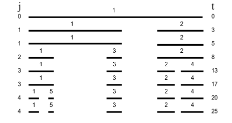
Figure 5: Schematic illustration of the construction of stochastic Cantor set. The numbers on the top of each intervals indicate their labels. The numbers on the left under $j$ indicates generation steps and the numbers under $t$ on the right illustrate how time evolves.

Figure 6: Decrease in the mean interval size $\delta$ as a function of time $t$. The straight line in the $\log(\delta)$ vs $\log(t)$ plot with slope equal to ${{1}\over{2}}$ implies that $\delta\sim t^{-{{1}\over{2}}}$ and hence it is in perfect agreement with analytical prediction.

The generalized master equation for the Cantor set given by Eq. (7) can describe the rules of the SCS problem stated in the algorithm (i)-(vii) if we choose

$$F(x,y|x+y+z)=1.$$ (24)

The master equation for the stochastic Cantor set then is

$${{\partial C(x,t)}\over{\partial t}}=-{{x^{2}}\over{2}}C(x,t)+2\int_{x}^{\infty}C(y,t)(y-x)dy.$$ (25)

This is exactly the rate equation first proposed and solved analytically by Krapivsky in the context of random car parking problem and later by an alternative method in the context of stochastic fractal ref.krapivsky ; ref.hassan . In this article, we however give an exact algorithm that can capture the complete dynamics described by the above rate equation and verify the analytical results by numerical simulation. Following the method of Krapivsky and Ben-Naim we incorporate the definition of the $n$th moment in the rate equation to give

$${{dM_{n}(t)}\over{dt}}=\Big{(}2{{\Gamma(n+1)\Gamma(2)}\over{\Gamma(n+3)}}-{{1}\over{2}}\Big{)}M_{n+2}(t),$$ (26)

and then solve it for $M_{n}(t)$. Following the same procedure as for the KCS problem we obtain the asymptotic solution for the $n$th moment

$$M_{n}(t)\sim t^{(n-0.56155)z}\hskip 9.95863pt{\rm with}\hskip 9.95863ptz=-{{1}\over{2}},$$ (27)

where the number $0.56155$ is the real positive root of the following quadratic equation

$$2{{\Gamma(n+1)\Gamma(2)}\over{\Gamma(n+3)}}={{1}\over{2}}.$$ (28)

Note that once again we find that the exponent of the power-law relation for $M_{n}(t)$ is linear in $n$ and hence the system must obey a simple scaling but only in the statistical sense. It is interesting to note that the moment of order $n=0.56155$, instead of $n=\ln 2/\ln 3$ in the KCS problem, is a consserved quantity. Using Eq. (10) in the definition of the mean interval size we find that

$$\delta(t)\sim t^{-{{1}\over{2}}}.$$ (29)

Once again we use it as the yard-stick and find that the number $N(\delta)$ needed to cover the resulting set scales as

$$N(\delta)\sim\delta^{-d_{f}},$$ (30)

where $d_{f}=0.56155$ is the fractal dimension of the stochastic Cantor set. It reveals that the fractal dimension of the stochastic Cantor set is less than that of its recursive or kinetic Cantor set.

Figure 7: Variation of the number of yard-sticks $N$ needed to cover the stochastic Cantor set is shown against the size of the yard-stick $\delta$. Data collected from simulation is averaged over $5000$ independent realizations. Slope of this straight line is found to be equal to $0.56155$ which means that $N(\delta)\sim\delta^{-0.56155}$.

Figure 8: The sum of the $d_{f}$th power of all the intervals $x_{1}^{d_{f}}+x_{2}^{d_{f}}+...+x_{j}^{d_{f}}=1$ regardless of time provided $d_{f}=0.56155$ which is the fractal dimension of the stochastic Cantor set. Data has been collected from the numerical simulation after averaging over $5000$ independent realizations.

To verify our analytical results we performed numerical simulation based on the algorithm $(i)-(vii)$. Note that the definition of time in this algorithm is very much different from that of the kinetic Cantor set. Like in the KCS problem here too we collect data for the mean interval size $\delta$ against time. We then plot $\log(\delta)$ versus $\log(t)$ in Fig. (6) and find straight line with slope equal ${{1}\over{2}}$. It implies that the mean interval size decreases following exactly in the same fashion as predicted by Eq. (29). We also collected data for $N$ against $\delta$. These data are used in Fig. (7) to show how the number $N$ decreases with the yard-stick size $\delta$. A straight line in the logarithmic scale with slope equal to $0.56155$ clearly implies that $N$ exhibits power-law relation $N\sim\delta^{-d_{f}}$ with exponent $d_{f}$ as predicted by Eq. (30). Furthermore, in Fig. (8) we show that the sum of the $d_{f}$th power of all the intervals

$$x_{1}^{0.56155}+x_{2}^{0.56155}+...+...+...\ +x_{j}^{0.56155}=1$$ (31)

regardless of the value of the generation step vis-a-vis the time. From the analytical point of view this is equivalent to the moment $M_{0.56155}$ of the distribution function $C(x,t)$ which is indeed found to be independent of time. All these results clearly reveals that analytical results are in perfect agreement with the numerical simulation.

V Summery

To summarize, in this article we studied two interesting variant of the strictly self-similar triadic Cantor set. We solved the two models, the kinetic and stochastic Cantor set, both analytically using rate equation approach and numerically based on the exact algorithms that we proposed for both the problems. We found that the number of intervals and time are related via a generalized relation $N\sim t^{d_{f}}$ is true for both kinetic and stochastic Cantor set if we set $d_{f}={{\ln 2}\over{\ln 3}}$ for the KCS problem $d_{f}=0.56155$ for the SCS problem. On the other hand, we found that the mean interval size decreases with time following power-law $\delta\sim t^{z}$ with exponent $z=1$ for the KCS problem and $Z={{1}\over{2}}$ for the SCS problem. We then took the respective mean interval size as the yard-stick to measure the resulting set and found that the number $N$ needed to cover the set fall-off following power-law with exponent equal to their respective fractal dimension. We also found a generalized conservation law in the sense that the sum of the $d_{f}$th power of all the available intervals at any time or the generation step is equal to the size of the initiator. This is true for recursive, kinetic and stochastic Cantor set. On the other hand, if we know the solution for the distribution function $C(x,t)$, which can only be defined for kinetic and stochastic Cantor set, then the conservation law means that the $d_{f}$th moment of $C(x,t)$ remain independent of time. It is noteworthy to mention that such non-trivial conservation laws was also found recently in the context of condensation-driven aggregation process ref.cda . We can perhaps conclude that emergence of fractal in a given system is always accompanied by some conservation laws which is ultimately responsible for fixing the various scaling exponents including the fractal dimension.

References

- (1) Mandelbrot B B, Fractals, 1977 Form, Chance, and Dimension (Freeman, San Francisco)
- (2) Mandelbrot B B, Fractals, 1982 The Fractal Geometry of Nature (Freeman, San Francisco)
- (3) Aguirre J, Viana R L, Sanjuan M A F, 2009 Rev. Mod. Phys. 81 333
- (4) Vicsek T, 1992 Fractal Growth Phenomena, 2nd ed. (World Scientific, Singapore)
- (5) Feder J, 1988 Fractals (Plenum Press, New York)
- (6) Newman M E J, 2005 Contemporary Physics, 46 323
- (7) Sears S, Soljacic M, Segev M, Krylov D, and Bergman D, 2000 Phys. Rev. Lett. 84 1902
- (8) Hatano N, 2005 J. Phys. Soc. Jpn. 74 3093
- (9) Krapivsky P L and Redner S, 2004 Am. J. Phys. 72 591
- (10) Esaki K, Sato M, Kohmoto M, 2009 Phys. Rev. E 79, 056226
- (11) Peitgen H-O, Juergens H, and Saupe D, 2004 Chaos and Fractals: New Frontiers of Science (Springer Verlag, New York)
- (12) Ziff R M and McGrady E D, 1986 Macromolecules 19 2513
- (13) Krapivsky P L, 1992 J. Stat. Phys. 69 125
- (14) Krapivsky P L and Ben-Naim E, 1994 Phys. Lett. A 196 168
- (15) Hassan M K, 1997 Physical Review E 55 5302
- (16) Hassan M K and Hassan M Z, 2009 Phys. Rev. E E 79 021406