Exploring pre-main sequence variables of ONC: The new variables

Abstract

Since 2004, we have been engaged in a long-term observing program to monitor young stellar objects in the Orion Nebula Cluster. We have collected about two thousands frames in V, R, and I broad-band filters on more than two hundred nights distributed over five consecutive observing seasons. The high-quality and time-extended photometric data give us an opportunity to address various phenomena associated with young stars. The prime motivations of this project are i) to explore various manifestations of stellar magnetic activity in very young low-mass stars; ii) to search for new pre-main sequence eclipsing binaries; and iii) to look for any EXor and FUor like transient activities associated with YSOs. Since this is the first paper on this program, we give a detailed description of the science drivers, the observation and the data reduction strategies as well. In addition to these, we also present a large number of new periodic variables detected from our first five years of time-series photometric data. Our study reveals that about 72% of CTTS in our FoV are periodic, whereas, the percentage of periodic WTTS is just 32%. This indicates that inhomogeneities patterns on the surface of CTTS of the ONC stars are much more stable than on WTTS. From our multi-year monitoring campaign we found that the photometric surveys based on single-season are incapable of identifying all periodic variables. And any study on evolution of angular momentum based on single-season surveys must be carried out with caution.

1 Introduction

The Orion Nebula Cluster (ONC) is an excellent target for studying young stellar objects (YSOs). It contains a few thousands of pre-main sequence (PMS) stars within $\sim$15 arc-minutes (2 pc) of the central Trapezium stars (Herbig & Terndrup 1986; Hillenbrand 1997; Hillenbrand & Hartmann 1998). At a distance, 450$\pm$70 pc, ONC is the nearest high-mass star-forming region where one can find very massive stars of $\sim$25 solar mass ($\theta^{1}$ Ori C) to sub-solar objects having mass well below the hydrogen burning limit (Hillenbrand 1997; Lucas & Roche 2000). From recent studies, it appears that formation of stars in the ONC started about 10 Myr back and, in the beginning, the formation process was very slow. Later, due to large scale contraction in the ONC parental cloud, the activity went through a rapid phase of star formation. The mean age of the ONC is about 1 Myr, which characterizes an epoch when large fraction of stars were born. An age spread of 2 Myr around this mean age is found by previous researchers (Hillenbrand 1997; Palla et al. 2005; Huff & Stahler 2006; Jeffries 2007). The ONC is located in front of a very extended and fully opaque molecular cloud (A_V peaks at 80-100 mag), which makes the background star contamination almost insignificant in the optical region. This means that except for a few foreground stars, all visible objects can be straight away considered to be cluster members. Very intense radiation pressure and stellar winds of the massive stars have cleared most of the dust from the ONC (O’Dell 2001) and that is why about 80% cluster members are subjected to relatively low visual extinction, A_V ranging from 0.0 to 2.5 mag (Hillenbrand 1997). The low-mass ONC stars are very strong sources of X ray emission and the median luminosity of these objects is L${}_{X}\sim 30.25$ erg sec^-1 (L_X/L_bol $\sim$10^-3.5), which is three orders of magnitude more intense than the solar X-ray luminosity (Flaccomio et al. 2003). Recent studies reveal that the X-ray luminosity of low-mass stars increases with the stellar mass and decreases with the age, but it seems to be independent of the rotation period (Flaccomio et al. 2003; Stassun et al. 2004; Preibisch et al. 2005).

In the past, for more than one decade, the ONC and the regions close-by (ONC flanking fields) were photometrically monitored by various researchers with varying degree of sensitivity as well as spatial coverage (Mandel & Herbst 1991; Attridge & Herbst 1992; Eaton et al. 1995; Choi & Herbst 1996; Stassun et al. 1999; Herbst et al. 2000; Carpenter et al. 2001; Rebull 2001; Herbst et al. 2002). Except the long-term observing program of Herbst and collaborators of Van Vleck Observatory (VVO) and near infra-red (NIR) survey carried out by Carpenter et al. (2001), other monitoring programs were primarily focused on a single goal and that was to explore the evolution of angular momentum of the stars in the PMS phase, by determining the rotation periods from the light curves produced by modulation of light due to hot/cool spots. We realized that moderate size telescopes equipped with wide field imaging camera can be very effectively used to address a variety of valuable scientific problems related to PMS stars. And hence using various observing facilities accessible to our group, since January 2004 we have initiated a long-term monitoring program on the PMS stars of the ONC. Since this is the first paper on this project, we not only report the results on the identification of new periodic variables but also describe the science drivers, the observation and the data reduction in some more detail. In Sect. 2 we describe our scientific motivations. Sect.  3 describes the selection of the target field and the observations. The data reduction procedures are described in Sect. 4 together with the tools used to determine very accurate rotation periods. In Sect. 5 we present the results on the newly discovered periodic variables. A brief discussion and our plan for the near future are given in Sect. 6.

2 Scientific Motivations

2.1 Exploring magnetic activities in T Tauri stars

T Tauri stars (TTS) are low-mass pre-main sequence objects and based on the strength of the H$\alpha$ line emission they are divided mainly into two sub classes: weak lined TTS (WTTS) and classical TTS (CTTS). The periodic photometric variability of WTTS is linked with rotational modulation of cool magnetic star-spots. Doppler Imaging, which is a robust stellar surface mapping technique, supports the cool spot model (Strassmeier 2002; Schmidt et al 2005; Skelly et al. 2008). WTTS are found to be relatively fast rotators with the preliminary indication that they do not possess surface differential rotation (Cohen et al. 2004; Skelly et al. 2008). They are sources of strong non-thermal radio as well as X-ray emission. Since T Tauri stars are believed to be fully convective, they cannot sustain the so-called $\alpha\omega$ interface dynamo. Furthermore, a fossil field can survive only over timescales from 10 to 100 years in a fully convective star. So, even for few-million-year-old TTS, a dynamo process is necessary to generate and amplify the magnetic field. The mechanism under which fully convective stars succeed to produce magnetism and related activities is a subject of debate (Chabrier & Kuker 2006 and references therein). The long-term monitoring of low-mass stars of the ONC will be very valuable to understand the mechanism responsible for the generation of magnetic field in fully convective very young stars. We are particularly interested to explore the presence/absence of activity cycles and of surface differential rotation in WTTS.

CTTS are surrounded by a circum-stellar accretion disk and are characterised by the presence of strong emission lines as well as an excess hot continuum emission. According magnetospheric models, strong dipolar field disrupt the inner disk at a few stellar radii. The disk material is channeled from the inner region of the disk onto the star along the magnetic field lines. The free falling material eventually hit the stellar surface and develops accretion shocks (Calvet & Gullbring 1998). The thermalized shock energy form hot spots/ring near the magnetic pole which is seen as an excess blue continuum emission in the spectrum of cool CTTS and in the optical-band photometry. The surface magnetic field measured from Zeeman broadening in several CTTS indeed indicates the presence of very strong magnetic fields with an average field strength of $\sim$2.5 kG (Johns-Krull 2007; Bouvier et al. 2007). Recent results from the Zeeman Doppler Imaging technique also reveal the presence of large-scale dipolar fields of about 1 kG together with a rather complex field configuration close to the stellar surface (Jardine et al. 2008; Donati et al. 2008). The hot spots are supposed to be foot prints on the photosphere of the large scale dipolar field, which facilitates the accretion from the disk. From our long-term multi-band monitoring program we intend to explore the temporal evolution of the hot spots. In addition, to obtain the disk accretion rate, we plan to model the CTTS light curves using star-spot models (Budding 1977; Dorren 1987; Mahdavi & Kenyon 1998) combined with the mechanism proposed by Calvet & Gullbring (1998) to account the excess emission coming from the hot spots.

2.2 Search for PMS eclipsing binaries

Eclipsing binary systems provide an opportunity to measure stellar masses, radii, effective surface temperature, and luminosity of the individual components with very high precision. These are the parameters one need to test various theoretical PMS evolutionary models. Several monitoring programs on young clusters, conducted recently by different groups have yielded only five such PMS eclipsing binaries (Irwin et al. 2007; Cargile 2008 and references therein). Therefore, the identification of more such systems is indeed in great demand. It appears that the discovery of just five eclipsing binaries among few thousand of PMS stars monitored so far, points toward the presence of some biases. The first thing we must take into account is that most of the surveys made in the recent past were single observing run, whereas the prominent source of variability in low-mass PMS stars are either due to the inhomogeneous distribution of cool/hot spots and/or to the variable disk extinction. Therefore, the shallower light variation due to the eclipses, being superimposed on these strong variations, is likely to be masked and only by means of repeated observations carried out over several seasons one can disentangle these effects. Moreover, all PMS eclipsing systems identified so far are Algol-type eclipsing variables. The close semidetached/contact binaries (if they can form) and partially eclipsing variables are simply indiscernible from single season light curves, and hence not have been identified so far. Therefore, from our continuous multi-year monitoring, we expect to identify a few more interesting candidates probably missed out by previous surveys.

2.3 Studying other interesting variables

UXor objects are mostly intermediate-mass PMS stars but can also be low-mass PMS stars. The light curves of these stars are characterized by sudden drops in brightness up to 3 mag in the V band, followed by increased reddening and linear polarization (Waters & Waelkens 1998; Grinin et al. 1998; Herbig 2008). In very deep minima the star reverses the color variation and, often, becomes bluer again (Bibo & The 1991). The origin of the brightness drops, the increase in polarization, and the blueing effect have been debated for a long time (Natta et al. 1997; Bertout 2000; Dullemond et al. 2003). The model based on variable obscuration suggest two different mechanism: passage of proto-cometary clouds in front of the star (Grady et al. 2000), and/or small hydrodynamic perturbations in the puffed-up inner rim (Dullemond et al. 2003, Pontoppidan et al. 2007). On the other hand, a very interesting mechanism was proposed by Herbst & Scevchenko (1999), in which unsteady accretion naturally explains several observable phenomena related to UXor. From several H$\alpha$ surveys including our own, we find about one hundred stars surrounded by the active accretion disk in our small FOV (Sect. 5.1), and it is quite expected that a few of these will indeed turn out to be UXor candidates.

FUor and EXor are young low-mass stellar objects surrounded by proto-planetary accretion disk and characterized by sudden enhancement in the luminosity. During eruption, an FUor star can be become 100 to 1000 times more luminous and, then after it gradually fades up, reaching a quiescence phase. On the other hand, EXor phenomenon is found to be less energetic but shows more frequent/recurrent transient activity. Both FUor and EXor phenomena are generally explained in terms of enhancement of disk accretion rate and several mechanisms have been proposed to trigger the outburst. These include a tidal interaction with a companion star, thermal or gravitational instabilities, and induced accretion due to presence of massive planets (Bonnell & Bastien 1992; Hartmann et al. 2004; Vorobyov & Basu 2005; Lodato & Clarke 2004). It is also not well understood whether the physical mechanism operating in EXor outburst is the same as in FUors and the difference in burst duration as well as the amplitude is a consequence of PMS evolution, or some very different physical process is responsible for the EXor phenomenon. There is one already known EXor in our field (V1118 Ori) and we expect to identify a few more EXor and FUor objects.

In addition to identifying such a new objects, our multi-band time series data together with the spectroscopic follow-up study will greatly help to understand the mechanism responsible for the UXor, FUor and EXor phenomenon.

2.4 The angular momentum evolution in the PMS phase

In addition to the above mentioned science objectives, our program will also be useful to address a few important aspects of the angular momentum evolution in the PMS phase. It is believed that a fraction of low-mass stars surrounded by disks goes through a phase of strong disk-braking, then after the disk-free star freely spins-up. The disk-braking models combined with the process of star formation (burst/sequential) as well disk dispersal, predict the bi-modal distribution of the rotation periods in young stars. However, numerous studies made on this regard over the last decade ended-up with very contradictory claims and counter claims (Stassun et al. 1999; Herbst et al. 2002; Rebull 2004; Lamm et al. 2005, Rebull 2006; Cieza & Baliber 2007). In most studies of stellar angular momentum, the stellar rotation period is obtained from light curves produced by the rotational modulation of the star light due to inhomogeneous cool/hot spots, unevenly distributed on the stellar surface. However, there have been no attempts made to check the completeness of the rotation periods derived from the light curves of various objects (except some work done by Cohen et al. 2004 on IC348; Lamm et al. 2005 on NGC2264). It is well known that the cool spots on WTTS and other active stars can change their size as well as spatial distribution so dramatically and rapidly that one can not expect to get always the rotation modulation, specifically when the amplitude of variation is small. That is the reason, for example, why the single-season survey made by Herbst et al. (2002) in 1998-1999 with the MPG/ESO 2.2m telescope could not detect all the bright periodic variables identified by the previous survey of Stassun et al. (1999), despite using a larger telescope and, hence, with better sensitivity and accuracy. On the other hand, stars with disks (mainly CTTS) are supposed to have both cool and hot spots. These stars usually display very irregular light variations and, often, it is difficult to get their rotation period accurately, at least from a single observing run (Herbst et al. 1994; Grankin et al. 2007). One of the question we want to address is why just about 10-20% of several thousands of low-mass PMS stars monitored so far are found to be periodic variables. What happened to the remaining 80-90% of stars? Why do they not show any regular and periodic variation despite having all the ingredients to produce magnetic spots? So, our long-term monitoring program hopefully will put us in the position to shed some light on detectability of the rotation periods and the effects of biases preventing their detections.

3 Selection of the field and Observation

3.1 The selection of the field

Keeping in mind the science goals mentioned in the preceding section, we started looking for a stellar field associated with very young stellar clusters containing a large number of confirmed and relatively bright young members confined to a small region. Another criterion was that the field must have a large number of already known PMS variables, representing to different mechanisms responsible for the light variations. Our search finally ended on the ONC, which was already chosen as target by other major monitoring programs, conducted by Stassun et al. (1999), Herbst et al. (2000), Rebull (2001), Carpenter et al. (2001), and Herbst et al. (2002). More importantly, since 1990 hundreds of bright stars of ONC have also been continuously monitored by Herbst and his collaborators of VVO. The field of view (FOV) of the telescopes what we planned to use was 10$\times$10 arc-minutes. Since our program needs long-term monitoring at least in two broad-band filters, and considering the limited availability of the telescope time, we had to further optimize a very potential 10$\times$10 arc-minutes field having large number of variables along with other measured quantities, such as NIR as well as X-ray data. We identified a region south west of the Trapezium stars shown in Fig. 1. The coordinate of the selected ONC field is $\alpha$(2000.0) = 05:35:04.09, $\delta$(2000.0) = $-$05:29:04.8. We deliberately kept the very bright trapezium stars out of the field, so that the strong scattered light and very severe bleeding of the charge should not spoil the CCD frame. The ONC field chosen by us includes 110 periodic variables already known from the literature: 92 from Herbst et al. (2000, 2002) and 38 stars from Stassun et al. (1999, hereafter called S99), where 20 periodic variables are common in both groups. The cross-correlation of optically-identified stars from Hillenbrand (1997), with 2MASS all sky catalogue of point sources (Cutri et al. 2003) and COUP X-ray observation (Getman et al. 2005), revealed that almost all optical stars have NIR counterparts and large number of them have X-ray data as well. Most of these objects are low-mass stars and extremely young candidates. Almost one fourth of our FOV is so close to Trapezium and severely affected by a strong HII region ( see Fig.1), whose average background level is several times larger than in the region slightly away from it. Nonetheless, we included this region because it hosts a large number of relatively young low-mass stars (younger than 1 Myr) and most of them have been found to be source of strong X-ray emission. Furthermore, it also comprises a large number of intermediate-mass stars (Hillenbrand 1997).

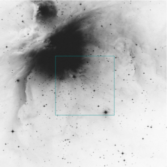
Figure 1: A $30\times 30$ arc-min red band image from DSS on which the $10\times 10$ arc-min region chosen for the long-term monitoring is marked.

3.2 Photometric Observations

The photometric observations of the ONC reported here, were obtained between January 18, 2004 and April 15, 2008, using the 2m Himalayan Chandra Telescope (HCT) and the 2.3m Vainu Bappu Telescope (VBT). The Himalaya Faint Object Spectrograph (HFOSC) of HCT used in imaging mode uses 2k$\times$2k central region of 2k$\times$4k CCD and covers a field of view of $10\times 10$ arc-minutes, with a scale of 0.296 arc-sec/pixel. The $1k\times 1k$ CCD mounted at the VBT prime focus covers a slightly larger field ($\sim$ 11$\times$11 arc-minutes) with plate scale of 0.65 arc-sec/pixel. The time series observations were made primarily through Bessel I & V broad-band filters. However, during the most recent observing run (2007-08) we collected time series observations in R band too. The most complete time series data in all observing runs is in I band. Reasons to give more emphasis to I band are: (i) the I band minimizes the effect of nebular background and interstellar extinction, as well it maximizes the S/N of red faint stars which constitute the bulk of the cluster population, (ii) past monitoring programs were conducted primarily in I band and so the comparison and the use of earlier data is only possible with I band, and finally (iii) the effect of the seeing is least in I band, and the effect of color dependent atmospheric extinction, which is difficult to correct, is also minimized. In order to avoid the degradation of seeing at low elevation, effort was also made to obtain photometric observations at low air-mass. Whenever possible, immediately after I band observations, we also tried to collect V & R band data with motivation to get the color curves of at least a few bright and less embedded cluster members. During the observing rus 2004-06, whenever telescope time was available, a sequence of 3-5 frames in each I and V filters with the exposure time of 60 and 180 seconds were collected. In order to increase the dynamic range as well as the photometric measurement accuracy of faint stars, starting from the most recent observing run (2007-08) we changed the observing strategy. Now, one short exposure is accompanied by 3-4 long exposures (20 and 90 seconds in I band, 60 and 300 seconds in V and R bands). Whenever possible, this observing sequence which finally gives one averaged data point was repeated more than once per night. In total the ONC field was observed on 208 nights and collected 1986 frames in R, V and I bands. A brief log of our observations is given in Table 1 and the distribution of the nightly observations for all the filters is shown in Fig. 2. The median seeing in I band for these observations is $\sim$1.5 arc-sec (FWHM) and, during the course of our observations, it varied from 0.8 to 2.5 arc-sec. Seeing at shorter wavelengths was slightly degraded according to the law of the wavelength dependent seeing (FHWM$\propto\lambda^{-1/5}$).

Since accurate flat fielding is of critical importance in differential photometry too, therefore, on every night we tried to collect a large number of evening and morning sufficiently-exposed twilight flats. Since there is no over-scan region in the detector used by us, several bias frames, spread over the night, were collected. It has been found that even after taking all sorts of precaution to do very accurate flat fielding, small errors of the order of 0.1 to 1.0% remain in the flat field (primarily due to non-uniform illumination of the flat field and wavelength-dependent differential variation in the quantum efficiency of the pixels). Furthermore, our back-illuminated thin CCD chips on both telescopes suffer from high spatial frequency fringing problem. The combination of these two effects typically limits the achievable photometric accuracy to a few milli-magnitude (mmag) depending on the instrument used. In order to minimize these effects, throughout the observing run, we tried to keep the stars in our FOV at the same pixel on CCD chip. To do this we selected a moderately bright star as a reference star and kept this star at reference pixel just before the closed loop guiding used to begin. During 90% of observations, all target objects were kept within the 2-3 pixels on the CCD frames.

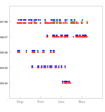
Figure 2: The distribution of the observed nights for all five cycles. The red, green and blue colors represent the observation made with I, R and V filters, respectively.

Table 1: Log of the observations made to date.

Cyc Start	Cyc End	Filter	No. Frames	No. Nights
Jan 18, 2004	Feb 16, 2004	I	121	16
		V	69	14
Oct 11, 2004	Jan 26, 2005	I	109	25
		V	80	22
Aug 26, 2005	Dec 22, 2005	I	89	21
		V	58	19
Nov 28, 2006	Apr 07, 2007	I	337	57
		V	159	38
Aug 25, 2007	Apr 18, 2008	I	492	89
		V	274	35
		R	198	50

3.3 Slit-less spectroscopy

In order to identify stars which show H$\alpha$ in emission, in a few observing nights of 2006-07, when the seeing was relatively better, the ONC field was also observed using HFOSC in the slit-less spectral mode with a grism as dispersing element. In this mode a combination of the H$\alpha$ broad-band filter (H$\alpha$-Br, 6100 - 6740$\AA$) and Grism 5 were used without any slit. This yields an image where the stars are replaced by their low-resolution spectra, which are on average displaced by 163 pixels upward in the CCD plane. The 2048$\times$2500 pixels, central region of the 2k$\times$4k CCD was used for data acquisition. The average dispersion of Grism 5 around H$\alpha$ is 3.12 Å/pixel and the seeing was around 1.2 arc-sec ($\sim$4 pixels), which sets the system resolution at about 500. Several repeated observations with 600 second were made on each night and bias as well as twilight flats were also taken on the same night with the same setup. After bias correction and the flat fielding, as done in the optical imaging, the spectral images were combined using median combine. The consecutive spectral images were taken while auto-guiding was active, so image shifts were found to be insignificant and stellar spectra after median combine were found to be not suffering through any smearing effect. On the other hand, we could improve not only the signal to noise ratio (S/N) in the median combined spectral image, but also remove the cosmic ray events and hence ensure unambiguous determination of sharp H$\alpha$ emission. From the median combined image, strips of the image containing the stellar spectra were copied and then the optimal extraction procedures carried out in slit-spectroscopy were followed. We used the IRAF task apall to extract the spectra of 346 stars. A very accurate sky subtraction from those stellar spectra which have been affected by the strong HII region is indeed very crucial. We sampled the sky from 2.5 arc-sec wide sky regions, nearly 2.5 arc-sec away, on either side of the stellar spectrum. To over come the problem of small scale strong variation in the sky background, a low-order polynomial was used to fit the background across the dispersion. This technique ensures that the nebular contribution in the H$\alpha$ profile is negligible and the measured H$\alpha$ emission is indeed coming from the star. The coarse wavelength calibration was done by using the average dispersion of the Grism 5, where the center of the H$\alpha$ line was used as a reference point (6562.8Å). The H$\alpha$ emission line stars were identified and the equivalent widths(EW) were measured. The smallest EW measured from our slit-less spectroscopy was found to depend on both seeing condition and star’s apparent magnitude. The later fixes the strength of the continuum, with respect to what we measure the EW of emission lines. On the seeing value smaller than 1.5 arc-sec, we could measure EW as small as 1Å   and this can also be considered the typical error in our EW for the stars having well exposed continuum.

4 Data reduction

4.1 Pre-processing and selection of the target stars

The basic image processing, such as bias subtraction and flat-fielding, were done in a standard way using tasks available within IRAF. In order to minimize the propagation of statistical errors while doing the bias subtraction and flat fielding, it is recommended that on each night one need to collect a large number of bias and flat frames . However, on average not more than 4-8 bias frames as well as twilight frames could be collected, due to the constraint imposed by long read-out time ($\sim$ 80 sec) of the CCD used. Therefore, to minimize the effect of propagation of the statistical error a large number of bias and flat frames were collected from near-by nights and, depending on the stability of the features on the frames, bias and flats of 3 to 4 consecutive nights were combined to construct the master bias and flat frames. After the bias correction and the flat fielding, the next task was to identify a large number of sufficiently bright stars in our field. To do this we selected one I-band frame which was obtained at fairly good seeing condition and used the daofind task of IRAF to identify stars within it. The radial profile of individual object was checked and the false detections or profile featuring extended objects were rejected. A total of 346 objects suitable for time series study were identified in this reference frame. Although the whole frame is affected to some extent by nebulosity, however, based on the intensity of the background emission we divided our FoV into three different sections, clear sky, sky partially affected by nebula and the region where the nebula is very strong. The stars falling in these regions were marked with the sky flags, SC, SPN and SN. In addition to this a SNB flag is used for bright stars located in the region where the nebular emission is strong. Nearly 5% of the frames taken under very poor sky transparency or worst seeing condition or affected by strong wind were rejected for subsequent analysis.

The astrometric calibration of the stars identified in the reference frame discussed above was done using the Starlink package ASTROM (Wallace 1994). The calibration was done using the coordinates of about one hundred stars listed in the 2MASS catalogue (Cutri et al. 2003) as references and on average the accuracy achieved on stellar coordinates is about 0.2 arc-sec. From the comparison with various coordinates reported by earlier researchers, it appears that our coordinates very well match with the coordinates of Herbst et al. (2002), with average difference of 0.23$\pm$0.21 arc-sec. Whereas, systematic 0.68$\pm$0.15 arc-sec and 1.39$\pm$0.28 arc-sec differences have been noticed with Hillenbrand (1997) and S99. Herbst et al. (2002) also reported such difference and it was found to be systematic errors in the astrometric transformation carried out by above two surveys.

4.2 The photometry

Despite our effort to keep our program stars always at the same CCD pixel, the observed frames were found to be typically out of the place and shifted with respect to the reference frame by 1 to 3 pixels. Furthermore, there were about 10% of the frames in which the effort was not made to center the star at the reference position on the CCD. So, before we start the photometric reduction we had two options. One possibility was to align all the frames with respect to a reference frame and to use the same coordinates obtained from reference frame to all the frames. The other possibility was to convert the coordinates of the stars determined from reference frame taking the image shift as well as the rotation into account. We opted the later procedure because the first procedure uses the intensity interpolation for the fractional shift in pixels and may not conserve the flux. The center of tens of bright stars were obtained using the CCD data reduction package DAOPHOT-II (Stetson 1987; 1992). Then after, the Stetson’s daomatch and the daomaster programs were used to obtain reasonably good transformation relation of stellar positions between the reference frame and any other observed frame. In the subsequent step the transformation relation generated by daomaster was used to generate an input coordinate file of all 346 stars whose coordinates have been already determined in the reference frame. This coordinate file was used as input to either aperture photometry carried out by the phot task of IRAF or the PSF photometry done using Stetson DAOPHOT-II.

For each star we performed both aperture as well as PSF photometry. In aperture photometry, the magnitude of stars were determined with aperture radius spanning the range of 4-10 pixels. Keeping relatively poor seeing in consideration (FWHM varies from 4 to 9 pixels), the sky was estimated from an annulus with slightly larger inner radius of 30 pixels ($\sim 8.8$ arc-sec) and width of 10 pixels. We played with various sky estimation procedures available in the IRAF and found that the mode gives more precise sky value and, hence, less scattered light curves of non-variable stars. Therefore, the sky was always estimated by using the mode option, whenever, aperture photometry was carried out. The PSF photometry was performed by modeling the star’s profile with a Penny-2 function. We used this function because we found it yield a least residual after subtracting fitted stars from the image. Besides the analytical functions, which are used for the fitting procedure, another important parameter of PSF photometry is the fitting-radius. For each frame we used a fitting-radius equal to the mean FWHM of the stellar profiles. Such a value was about 4 pixels for the images acquired in good seeing and about 8 pixels in poor seeing conditions. If any faint object has bright neighbours, then the effects of variable seeing combined to the intrinsic variability of the bright neighbours can introduce spurious variations. Such close pairs were identified and their time series photometric data was treated with special care. On total we identified 17 such pairs which have been found to be separated by less than 6 arc-sec.

4.3 Ensemble differential photometry

The differential photometry was performed using the technique of ensemble photometry (Gilliland & Brown 1988; Everett & Howell 2001; Bailer-Jones & Mundt 2001). In ensemble photometry the differential magnitude is computed with respect to the average magnitude of a large number of non-variable reference stars. The advantage of this technique is that, in the averaging process, the uncertainties of the ensemble stars magnitudes due to statistical fluctuations as well as short-term small incoherent variations will cancel each other. The uncertainty in the magnitude of the artificial comparison, therefore will be smaller than the uncertainty on the magnitude of a single star and this, in turn, will produce less noisy light curves. The ensemble photometry was performed with ARCO, a software for Automatic Reduction of CCD Observations, developed by us (Distefano et al. 2007). This software allows us to select automatically the suitable stars for the ensemble, i.e., sufficiently bright and isolated stars, which are common to all the frames, and distributed all over the frame but not found to be close to the CCD edges. After selecting the ensemble stars, ARCO automatically computes: (i) the magnitude of the artificial comparison star by averaging instrumental flux of ensemble stars, (ii) time-series differential magnitudes for each star of the field and (iii) mean, median and the standard deviation ($\sigma$) associated to each time series. While computing the average ensemble magnitude, we first determined the average flux of all ensemble stars and, then after, the ensemble magnitude was computed from the average flux. This way of computing ensemble magnitude gives more weight to the bright stars which are expected to have smaller error related to photon noise.

The whole procedure described above is iterative and start with a large number of bright stars distributed all over the frame, excluding stars very much affected by the nebulosity. While constructing the ensemble, the program exclude those ensemble stars whose standard deviation is larger than the threshold sigma value fixed by the user. The final output of the software is a file with differential time-series magnitudes for all stars in the field including the ensemble stars. We used the ensemble made up of 24 stars to get differential magnitudes in I, R and V photometric bands. We run the program several times with different input data coming from apertures as well from PSF photometry and generated several sets of light curves.

In principle, when differential aperture photometry is performed, the choice of the radius should not matter because, if the stellar profile does not vary significantly across the frame, the percentage of the total flux collected through an aperture of a given radius $r$ is same for all stars and, therefore, there should be no difference between time-series data obtained with a 4-pixel aperture radius or with an 8-pixel radius. However, the use of a fixed radius for all stars is not recommended when the stars of the field span a broad range of magnitudes. Although a larger aperture increases the signal strength, however, at the same time, it increases the contribution of the noise due to the background fluctuations and CCD read out. In the case of bright stars the contribution to the total noise is mostly the photon noise whereas, the noise in the faint star magnitude is due to the sky and read out noise of the CCD. So, a large aperture is preferable to bright stars and a smaller aperture to faint stars. It is well known that signal-to-noise ratio is a function of size of the apertures and is found to be maximum close the aperture radius of one FWHM of the stellar profile (Howell 1989). The magnitude of faint stars may be very much affected even by slight inaccurate estimation of sky values and this can be minimized by adopting a small aperture. Whereas, any variation in the shape of PSF over the frame introduces error in the bright stars magnitudes. Keeping all these in mind, a range of apertures starting from 4 to 8 pixels were used to generate the ensemble differential photometry.

As mentioned in Sect. 3, the differential ensemble magnitudes of the sequence of 3 to 4 frames collected within very short intervals of time (shorter than 1 hour) were combined and the mean value of the magnitudes from these close-by frames was used as one data point in the time series analysis. We also computed standard deviation of these magnitudes which is a robust estimate of the error associated with each data point. The mean of the standard deviation $<\sigma>$ is an average error of the measurement associated with any star which is a function of the magnitude and plotted in the Fig. 3. Such an estimate of error linked with one data point is conservative because the true observational accuracy could be, in principle, even better for stars having substantial variability within the timescale close to our fixed binning time interval (i.e. 1 hour). We have computed the mean error $<\sigma>$ for all three apertures of radius 4, 6 and 8 pixels, respectively. The lower bounds of the data points were fitted with a piecewise function of second order polynomials and the exponential function (see Fig. 3). As expected, the smaller apertures give better photometric precision to the faint stars. Whereas, the large apertures seem to be more suitable for the brights stars. Relatively large errors associated with the magnitudes determined using small aperture of bright stars reflect the effect of temporal as well as spatial variation of the PSF. The photometric precision achieved in the interval of 11.5$<$I$<$16.0 is close to 0.01 ($\sim$1%) and then it degrades exponentially. During the final run of the photometric reduction, the optimum aperture was not only selected based on the stars brightness, but the aperture which gives the lowest mean error ( $<\sigma>$) was also taken in to account.

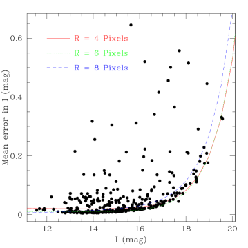
Figure 3: The mean error associated to each data points as function of the I band magnitude. The sequence which comprises the maximum distribution of the data points, were fitted with a piecewise function of second order polynomials and the exponential function. The data points of aperture radius 6 has been only plotted here, but fitting were done for data of all three apertures 4, 6 and 8 pixels radius and the best fit curves are shown here. Most of the deviant data points with respect to the fit, are associated with the stars in strong nebula and hence the background photon noise are the prime source of the error.

Finally, we performed a comparison between the results obtained from aperture photometry and from PSF-photometry. Such a comparison is shown in Fig. 4, where $\sigma_{8}-\sigma_{psf}$ and $\sigma_{4}-\sigma_{psf}$ vs. I mag are plotted. In the fainter domain PSF-photometry is more advantageous than aperture photometry carried out with 8-pixel radius (Fig. 4). However, if the aperture photometry is done with radius of four pixels, then aperture photometry gives better results in the fainter domain (Fig. 4). From all these detailed exercise we found that in our case generally the aperture photometry is more advantageous than PSF-photometry. Nevertheless, we found that there are few stars for which PSF-photometry produces less noisy light curves and we noticed that such stars are either close to a brighter star or lying close to edges of the CCD. In such cases PSF-photometry is more efficient because it allows us to take into account the effects of the distortion of the stellar profile at the edges of CCD as well as it ”deblends” the star from the brighter neighbours. Therefore, to construct time series data of these stars we used PSF-photometry.

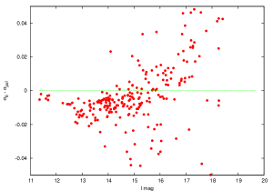
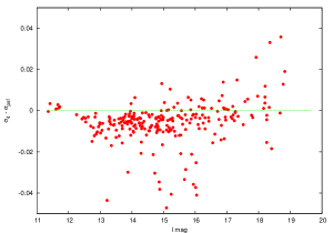
Figure 4: In the top panel the quantity ”$\sigma_{8}-\sigma_{psf}$” vs. the I magnitude is plotted. The radius of 8 pixels gives a smaller standard deviation and, in turn, a less noisy light curve for brighter stars. To the fainter stars PSF photometry seems to be advantageous, but looking at the $\sigma_{4}-\sigma_{PSF}$ vs. I mag plot (bottom panel), it appears that also in such a case aperture photometry gives the better results.

4.4 Absolute Photometry

In order to obtain the standard magnitudes and the colors of all targets in our FOV, which allow our observations to compare with previous observations, we decided to carry out photometric calibration as precise as possible. The standardization of magnitudes also enables us to correctly place our objects in the HR diagram and to determine various stellar parameters. On the six best nights of the 2007-08 observing run, we observed a large number of BVRI photometric standard stars from Landolt (1992) and deeper asterism of M67 (Anupama et al. 1994). A few Landolt fields were monitored over a wide range of air-mass to determine the nightly atmospheric extinction. From the extinction observation we found that only four out of six nights were photometric and the transformation coefficients were obtained from these nights. On the same night a large number of VRI frames with short and long exposures of the ONC were taken, when it was close to the meridian. The short and long ONC frames were aligned and then co-added separately, using the median option of the imcombine task of IRAF. The aperture photometry magnitude with a radius of 1.5$\times$FWHM, which is suppose to give maximum S/N was carried out for the all 346 ONC variables. Then after, 20-30 fairly isolated bright stars free from nebulosity were used to determine the aperture correction. Finally the aperture corrected magnitudes of the ONC stars were obtained for the aperture of 5$\times$FWHM and then I-band magnitude and colors were transformed using the transformation equation

$$I=i-k_{i}X+\epsilon(R-I)+\zeta_{i}$$ (1)

$$(R-I)=((r-i)-k_{ri}\Delta~{}X)\mu_{ri}+\zeta_{ri}$$ (2)

$$(V-I)=((v-i)-k_{vi}\Delta~{}X)\mu_{vi}+\zeta_{vi}$$ (3)

where k, X, $\epsilon$, $\mu$ and $\zeta$ are atmospheric extinction, air-mass, transformation coefficients, and zero points, respectively. The average magnitude and colors of all 346 stars were obtained from four nights using Eq. (1-3).

Finally, the accuracy of the photometric calibration was estimated by computing the standard deviation of magnitudes and colors of the 24 comparisons used for the differential ensemble photometry. And the errors were found to be 0.02, 0.04, and 0.05 mag in I band, (R$-$I) and (V$-$I) colors, respectively. Because, nearly all stars in our field are expected to be variable with amplitude of variability in the range from our accuracy limit (0.01mag) to few tens of magnitudes, therefore, a better estimate of their brightness comes from the mean/median value of the time series data. Therefore, we determined the median magnitudes of each star’s time series data collected over five consecutive observing years and compared these values with the I-band magnitudes of Hillenbrand (1997) and Herbst et. al (2002), the latter collected during a complete observation season. The difference of the median magnitudes obtained from the common stars are plotted against our I-band magnitude in Fig. 5. Our median magnitudes and those from Herbst et al. (2002) seem to matching well, whereas, the difference with respect to Hillenbrand (1997) is quite apparent in the plot. Here we remind that, differently than Herbst et al. (2002), the photometric data used by Hillenbrand (1997) was mostly based on snapshot observations collected over few nights and hence affected by the intrinsic variability. The photometric data along with other relevant information of all 346 stars in our FOV are partly given in Table 2, whereas, the complete table is available only electronically.

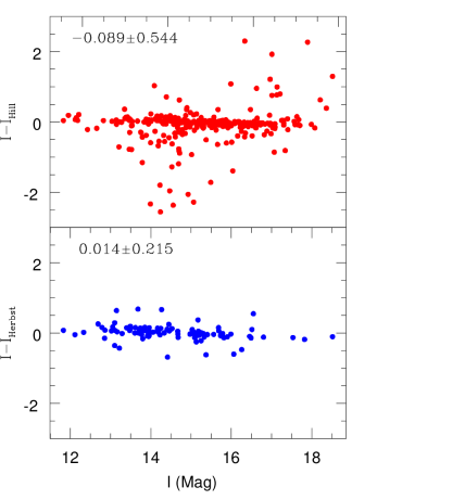
Figure 5: The comparison of I-band magnitudes obtained from our photometry and from Hillenbrand (1997), and Herbst et al. (2002). The mean and the standard deviations of the difference in magnitudes are also given on the top of each plots.

Table 2: The photometric data along with other relevant information of all 346 stars in our FoV.

S.N.	RA-Dec	JW	PHerbst	PStassun	Sky	Neighbour	CTTS	I	R-I	V-I	Sp.Type	J	J-H	H-K	LX
161	05 34 55.006 -05 26 58.90	3111	-	-	SC	-	-	16.07	1.44	3.22	M5.5e	13.83	0.92	0.61	29.00
162	05 34 53.100 -05 26 59.54	-	-	-	SC	-	-	18.61	3.60	2.67	-	15.96	0.79	0.35	28.04
163	05 34 50.727 -05 27 01.01	117	8.870	-	SC	-	C	13.17	1.02	2.10	M0e	11.65	0.93	0.53	29.26
164	05 35 21.627 -05 26 57.78	688	-	-	SPN	-	-	14.68	0.74	2.81	-	12.84	0.76	0.31	29.10
165	05 35 05.851 -05 27 01.64	281	3.160	-	SPN	-	-	13.95	1.78	3.29	M3.5	12.10	0.96	0.32	29.56
166	05 35 06.426 -05 27 04.82	290	-	-	SPN	-	-	15.37	1.56	3.81	-	12.93	0.74	0.48	29.41
167	05 35 05.891 -05 27 09.00	283	7.010	-	SPN	-	-	15.19	0.48	2.79	K8	12.51	1.37	0.75	29.72
NOTE: Only a portion of the table is shown here and complete table is available only in electronic edition of the MNRAS.

4.5 Search for periodicity

As already mentioned, one major objective of our project is to detect and characterize the optical and NIR band variability of all targets detected in our FOV. Specifically, we aim at discovering new variables and their rotation period whenever possible. The variability of low-mass members of ONC mostly arises from uneven distribution of cool/hot brightness inhomogeneities on the stellar photosphere, which, being carried in and out of view by the star’s rotation, produce a quasi-periodic variation in the observed flux. The variation in the star’s light is modeled through Fourier analysis to determine the stellar rotation period. There are transient phenomena related to magnetic activity, such as flaring and micro-flaring, and star-disk interaction which also give rise to flux variability. However, they generally tend to be non-periodic, making more difficult the detection of any periodicity in the observed time series data. The reliable determination of the stellar rotation period is possible if several conditions are met at a time. For example, stars must have surface inhomogeneities unevenly distributed along the stellar longitude, the stellar latitude of spots in combination with the inclination of the rotation axis must allow the rotation to modulate the spot visibility, and the inhomogeneity pattern must be stable over the time interval when the photometric data are collected. Finally, the non-periodic phenomena mentioned earlier should not be dominant contributors to the flux variation. All these conditions are not always satisfied.

Most of our targets are either WTTS or CTTS which show in some respects different patterns of variability. In the case of WTTS, the observed variability is dominated by phenomena related to magnetic activity which manifest themselves on different time scales, as it also occurs in the more evolved MS and post-MS late-type stars (see Messina et al. 2004). The shortest time scale, of the order of seconds to minutes, is related to micro-flaring activity. Its stochastic nature increases the level of intrinsic noise in the observed time series flux. The variability on time scales from several hours to days is mostly related to the star’s rotation. Whereas, the variabilities on longer time scales, from months to years, are related to the growth and decay of active regions (ARGD) as well as to the presence of star-spot cycles. In order to differentiate the effects on the variability by ARGD and star-spot cycles from the effect of rotation, on which we are presently focused, we have analyzed our time series data season by season from 2004 to 2008. Excluding cycle 5 which is currently the longest one, we have collected our data during observation seasons which are shorter than the timescale of ARGD typically observed in PMS stars. In the case of CTTS, apart from cool spots, also hot spots formed by accretion from the disk introduce additional variability. This type of variability is quite unexplored, in the sense that our knowledge either of the accretion processes or of their time scales is not as good as for WTTS. We know from previous studies that in most cases the combination of different mechanisms operating on different time scales makes the variability highly irregular.

We included in our analysis also the data collected by Herbst et al. (2002) (hereafter referred to as H02), kindly made available to us on our request. The independent analysis of the H02 data with our tools (described in the following subsections), allowed us to check the reliability of our period search procedures. We first searched for the periodicity in our I band time series data collected over all the seasons, because the I band data are more numerous than V as well as R band data (see Fig. 2 and Table 1) and also have greater S/N ratio. Afterwards, the analysis of R and V band time series data was carried out to either confirm the periodicity found from the I-band data and/or to search for additional periodic variables.

We have used the Scargle-Press periodogram to search for significant periodicity. In the following sub-sections we briefly describe our procedures to identify periodic variables among our targets.

4.6 Scargle-Press periodogram

The Scargle technique has been developed in order to search for significant periodicities in unevenly sampled data (Scargle 1982; Horne & Baliunas 1986). The algorithm calculates the normalized power P_N($\omega$) for a given angular frequency $\omega=2\pi\nu$. The highest peaks in the calculated power spectrum (periodogram) correspond to the candidate periodicities in the analyzed time series data. In order to determine the significance level of any candidate periodic signal, the height of the corresponding power peak is related with a false alarm probability (FAP), which is a probability that a peak of given height is due to simply statistical variations, i.e. to noise. This method assumes that each observed data point is independent from the others. However, this is not strictly true for our time series data consisting of data consecutively collected within the same night and with a time sampling much shorter than the timescales of periodic variability we are looking for (P^d=0.1-20). The impact of this correlation on the period determination has been highlighted by, e.g., Herbst & Wittenmyer (1996), S99, Rebull (2001) and Lamm et al. (2004). In order to overcome this problem, we decided to determine the FAP by different ways than proposed by Scargle (1982) and Horne & Baliunas (1986), the latter being only based on the number of independent frequencies. We followed the method opted by H02 (hereafter referred to as Method A) and the approach proposed by Rebull (2001) (hereafter referred to as Method B) .

4.6.1 Method A

Following the approach outlined by H02, randomized time series data sets were created by randomly scrambling the day number of the Julian day (JD) while keeping photometric magnitudes and the decimal part of the JD unchanged. This method preserves any correlation that exists in the original data set. We noticed that Lamm et al. (2004) in order to produce the simulated light curves, randomized the observed magnitudes, instead of the epochs of observation. Then after, we applied the periodogram analysis to the ”randomized” time series data for a total of about 10,000 simulations. We retained the highest power peak and the corresponding period of each computed periodogram. In the top panel of Fig. 6, we plot the distribution of detected periods from our simulations for I- band data of the 5th cycle, whereas, in the bottom panel we plot the distribution of the highest power peaks vs. period. The dashed line shows the power level corresponding to the 99% confidence level. The FAP related to a given power P_N is taken as the fraction of randomised light curves that have the highest power peak exceeding P_N which, in turn, is the probability that a peak of this height is simply due to statistical variations, i.e. white noise. We note that such power thresholds are different from season to season, because of different time sampling, length of the observation season, and total number of data. The normalised powers corresponding to a FAP $<$ 0.01 are reported in the second column of Table 3 for the 5 observation seasons as well as the averaged H02 data. We note that in our analysis we averaged the H02 time series data in the same manner as done in our own time series (see Sect. 4.3). Therefore, the reduced total number of analysed data in each light curve leaded to a proportionally smaller power level - about 8.2 against 16.5 for the unaveraged data as reported by H02.

Table 3: Normalized power at 1% FAP as established by randomizing time series (Method A) and by correlated Gaussian noise (Method B)

cycle	Method A	Method B
		Lcorr(d)
		0.0	0.1	0.25	0.5	1.0	2.0
	PN	PN	PN	PN	PN	PN	PN
1	6.2	7.0	8.2	9.1	9.3	9.5	10.4
2	6.9	7.8	7.9	8.3	9.2	9.9	10.3
3	6.6	7.3	7.7	7.6	7.7	7.6	8.6
4	8.4	8.0	8.8	9.6	10.3	11.4	13.4
5	9.2	8.4	11.4	13.9	15.5	16.7	19.6
H02 (averaged)	8.2	7.8	8.2	8.8	9.4	10.4	12.8

4.6.2 Method B

Following the method given by Brown et al. (1996), synthetic time series data was generated with the same sampling as the observed data and the frequencies were searched over the same range as done with the real data. The synthetic time series are built by using a random number generator with a Gaussian distribution of points

$$x_{i>0}=\alpha x_{i-1}+\beta R(0,\sigma)$$ (4)

where $x$ represents the magnitude of the light curve, $\alpha$=exp($-\Delta$ t/L_corr), where $\Delta$t is the time between magnitudes x_i-1 and x_i, $\beta$=(1$-\alpha^{2})^{1/2}$, and R(0,$\sigma$) is the random number generator with a dispersion $\sigma$, which is the variance of the time series data. The initial mean magnitude $x_{0}$ is selected via a call to R(0,$\sigma$). For more details on this procedure see Rebull (2001) and Brown et al. (1996). L${}_{corr}=0$ d sets the case of uncorrelated Gaussian noise, where each data is assumed to be uncorrelated from others. A range of correlation time starting from 0.1 to 2 days were used. For each value of correlation time we have built a set of about 10000 synthetic light curves and used the distribution of maximum power from the corresponding periodograms to determine the 1% FAP. The results are summarized in Table 3.

The increase of L_corr implies that the synthetic light curves become more correlated and this makes the power level corresponding to any threshold FAP larger, which in turn increases the risk to miss the detection of real periodicities. We found that a value of L_corr=1.0d is a good compromise to properly account for the correlation in our data. For L${}_{corr}>$1.0d we start systematically missing even those rotation periods whose reliability have been firmly established by previous multi-year surveys (e.g. H00).

We see that the power level adopted to discriminate periodic from non periodic target is larger than the values found both in the Method A and in Method B for uncorrelated Gaussian noise (L${}_{corr}=0.0$d). Finally, we notice that these FAP values are conservative. The reason is that even in the same observing run the sampling of the time series data differ from object to object. This happens primarily due to, objects close to the edge of the detector were some time missed out due to telescope pointing error, some time at poor seeing faint objects failed to collect sufficient signal and hence undetectable. When doing our simulations we adopted the largest FAP level, which we generally found in the most numerous time series data (that is the case for more than 80% of light curves).

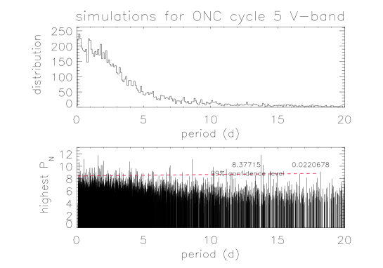
Figure 6: Distribution of periods (top panel ) and power of the highest peaks (bottom panel ) resulting from Scargle periodogram analysis of 10,000 ”randomised” light curves. Original time series data were collected during cycle 5 in the I band.

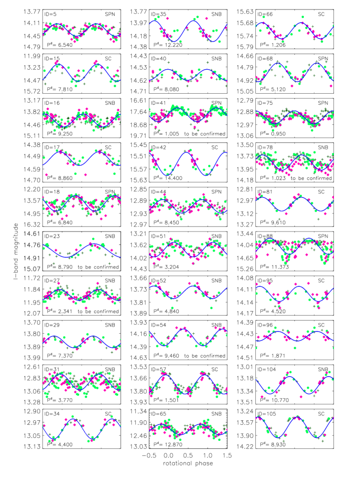
Figure 13: I-band light curves of our periodic variables vs. rotation phase. Phases are computed using the rotation period reported in Table 5. Different symbols are used to disctinguish data belonging to different time intervals (see caption of Fig. 9. The solid line represents the sinusoidal fit to the data.

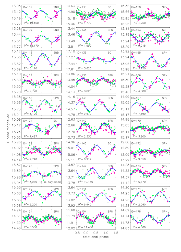
Figure 14: continued.

In order to establish whether a star can be considered a periodic at 99% confidence level we decided to adopt Method B for correlated Gaussian noise (L${}_{corr}=1.0$d). All the stars listed in Table 5 satisfy this selection criterion. In a few cases, as shown in the on-line Figs.8-14, more than one peak were found with power exceeding the fixed threshold value at 99%. These secondary peaks are generally alias of the peak related to the rotation period, which is the only periodicity we expect in these late-type PMS stars in the period range searched by us (0.1-20 days). In order to check that the secondary peaks are indeed nothing but an aliasing effect as well as to correctly identify the rotation period, we proceeded by subtracting the smooth phased light curve of period associated with highest peak. Then after, we re-computed the periodogram on the pre-whitened time series data. In most cases no significant peaks were left in the pre-whitened time series data with confidence level larger than 99%. A total 14 stars whose rotation periods were detected with a confidence level larger than 99% were excluded from the following analysis and not included in Table 5, since they display very noisy phased light curves. These stars were also not identified as a periodic variables by previous surveys.

4.7 Uncertainty with the rotation period

In order to compute the error associated with periods determined by us we followed the method used by Lamm et al. (2004). According to this method the uncertainty in the period can be written as

$$\Delta P=\frac{\delta\nu P^{2}}{2}$$ (5)

where $\delta\nu$ is the finite frequency resolution of the power spectrum and is equal to the full width at half maximum of the main peak of the window function w($\nu$). If the time sampling is not too non-uniform, which is the case of our observations, then $\delta\nu\simeq 1/T$, where T is the total time span of the observations. From Eq. 5 it is clear that the uncertainty in the determined period, not only depend on the frequency resolution (total time span) but is also proportional to the square of the power. We also computed the error on the period following the prescription suggested by the Horne & Baliunas (1986) which is based on the formulation given by Kovacs (1981). We noticed that the uncertainty in period computed according to Eq. 5 was found to be factor 5-10 larger than the uncertainty computed by the technique of Horne & Baliunas (1986). In this paper we report the error computed with the first method described above. Hence, it can be considered as an upper limit, and the precision in the period could be better than that we quote in this paper.

5 Results

5.1 The H$\alpha$ line emission stars

The strong H$\alpha$ emission coming from low-mass PMS stars is an unambiguous signature of active accretion from the disk on to the surface of star. Reliable knowledge of the presence/absence of a accretion disk is desirable particularly for studying evolution of the angular momentum in the PMS phase. Moreover, it helps us to better treat the light curves of these stars which arise either from compact hot-spots and/or from the variable extinction introduced by inhomogeneous distribution of the disk material. Information about H$\alpha$ emission of stars in our field of view come either from old objective prism surveys (Haro 1953; Wiramihardja et al. 1991) or from the recent surveys made by using multi-object spectrographs (S99; Sicilia-Aguilar et al. 2005; Furesz et al. 2008). These surveys are not complete. The old objective prism surveys suffer from sensitivity and were unable to obtain reliable information about the H$\alpha$ emission from faint stars. The surveys made with multi-object spectrographs consist of pointed observations and, primarily, suffer from selection effect, i.e. the number of fibers were limited and, hence, not all the ONC PMS could be included in these surveys. Therefore, we decided to do a deep slit-less spectroscopy to identify the H$\alpha$ emitting stars in our ONC field. Details about the observations and the data reduction were given in Sect. 3.3. From our slit-less spectroscopic survey we could identify a total of 40 emission lines stars with moderate to very large H$\alpha$ equivalent widths. The EW of these emission line stars together with other relevant informations are given in Table 4. Of these 40 stars, 13 stars were not reported by the surveys mentioned above. The spectra around H$\alpha$ are shown in Fig. 7. The very recent survey carried out by Furesz et al. (2008) has newly detected a large number of H$\alpha$ emitting stars. These stars are found to have CTTS-like H$\alpha$ emission with wide wings or asymmetric profile under the strong nebular component. Likewise objective prism survey, our slit-less survey suffers from the problem of high sky background. However, by adding several frames, doing accurate sky subtraction and, finally, making use of optimal spectral extraction, we could obtain useful spectra of stars as faint as 16 mag in I band, and 18 mag in V band. Interestingly, we could not detect H$\alpha$ emission in very few cases, although such stars were bright and previously reported as strong H$\alpha$ emitters. We have also listed such stars in Table 4. Altogether, 96 stars have been found to be H$\alpha$ emitting stars in our small FOV and most of these H$\alpha$ emitting stars belong to low-mass CTTS group.

Table 4: The list of stars showing H$\alpha$ line in emission. We also present stars previously found to be strong H$\alpha$ emitter but not in our survey.

ID	JW	EW(Å)	Period	Sky	I(mag)	Sp-Type
5	265	-59.28	6.54	SPN	14.26	-
81	123	-19.77	9.61	SC	12.85	K2
136	245	-42.90	8.82	SPN	13.91	M2e
163	117	-34.90	9.01	SC	13.17	M0e
172	288	-11.65	9.85	SPN	13.02	-
184	272	-58.19	2.98	SC	14.16	M1.5e
206	580	-908.19	—-	SPN	16.56	M1:e
209	320	-76.24	—-	SC	14.74	K2
225	138	-87.67	4.34	SC	14.67	M3.5e
227	107	-168.31	1.07	SC	14.13	M1.5e
229	239	-12.75	4.46	SC	12.79	M2.7
239	277	-462.06	—-	SC	15.29	-
242	235	-106.40	—-	SC	13.77	-
244	576	-5.54	1.95	SC	13.13	M1.5
250	135	-18.39	3.67	SC	13.77	M3e
263	379	-35.37	5.59	SC	15.19	M5.2
270	381	-74.05	7.75	SC	13.96	-
271	632	-45.21	3.77	SC	15.31	M5.5
272	628	-42.33	2.25	SC	14.23	-
273	647	-68.09	8.20	SC	13.36	M5e
276	91	-13.60	16.67	SC	13.49	M4
278	416	-14.01	2.11	SC	14.16	M3.5
282	421	-13.26	8.84	SC	11.67	G7:e
290	294	-35.78	2.57	SC	15.41	M4.5
295	715	-92.38	—-	SC	15.21	M5.5
296	673	-11.76	3.22	SC	13.11	M5
299	165	-4.70	5.74	SC	11.85	A7
303	101	-33.50	1.05	SC	14.42	G:e
304	328	-48.73	—-	SC	12.80	K4
310	518	-94.63	—-	SC	15.00	-
313	649	-88.45	1.80	SC	15.69	M6
320	313	-26.15	—-	SC	13.40	M0
321	447	-30.78	2.60	SC	15.17	M4
326	5159	-88.01	2.39	SC	17.07	-
328	498	-9.97	7.27	SC	13.95	-
332	225	-11.28	—-	SC	13.60	M1.5
333	501	-4.79	9.69	SC	13.14	M0
339	295	-126.44	2.85	SC	13.15	M2
342	73	-142.96	2.23	SC	14.45	M1e
346	284	-76.49	3.08	SC	14.17	M3e
			No H$\alpha$
18	278	-59.0	6.84	SPN	13.84	K4:e
45	127	-43.0	—-	SC	13.9	-
105	192	-25.0	8.93	SC	13.77	M2
148	258	-20.0	9.94	SPN	13.8	M0.5
204	334	-65.0	5.34	SC	14.27	-
216	422	-22.0	5.94	SC	14.46	-
327	115	-86.0	—-	SC	15.99	M5.5

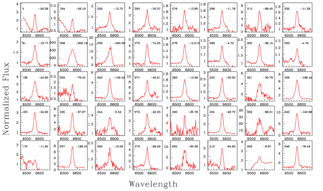
Figure 7: The spectra around H$\alpha$ from slit-less spectroscopic observations made on February 07, 2007 using HFOSC.

5.2 The color-magnitude diagram

The color-magnitude diagram (HR diagram) is the most reliable and widely used tool to obtain mass, age, and radius of cluster members. These fundamental stellar parameters are determined by comparing the position of stars on HR diagram with pre-main sequence evolutionary tracks. Furthermore, the distribution of stars with respect to PMS isochrones may reflect the star formation history (Lada & Lada 2003). It is also an effective tool to explore the evolution of stellar angular momentum in the PMS phase. To construct the HR diagram we need very accurate measurements of effective temperatures (colors) as well as of luminosities (magnitudes) of stars. The precise effective temperature is usually measured from spectroscopy, whereas, the luminosity is obtained from de-reddened as well as bolometric corrected magnitudes. The spectral coverage and resolution of our slit-less spectra does not allow us to obtain accurate spectral type, and hence as the temperature, or equivalently, the intrinsic color is concern we rely on Hillenbrand (1997) data. On the other hand, much more accurate I and V band magnitudes are determined from our own long-term observations. The median value determined from the data of all five cycles is expected to be less affected by the astrophysical error (Hillenbrand 1997). The I vs. V$-$I color-magnitude diagrams, before and after inter-stellar extinction correction, are given in Fig. 8. The A_V and (V-I)_o, which are taken from Hillenbrand (1997) are available for only 50% of our program stars. Therefore, the reddening corrected CMD could be only made for a sub-sample of our data. We have also over-plotted the ZAMS and various isochrones from Siess et al. (2000). The solar metallicity with no convection overshooting was used to compute the ZAMS and the isochrones. The theoretical effective temperatures and luminosities were converted into (V$-$I) color and V and I magnitudes by making use of the conversion tables of Kenyon & Hartmann (1995).

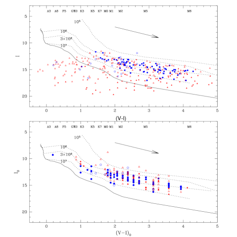
Figure 8: The color-magnitude diagram of ONC stars without reddening correction is shown in the top panel. The bottom panel shows the same diagram after reddening correction. Filled and open data points represent stars inside or outside nebulosity, respectively. The circles represent CTTS and other stars are marked by a triangle.

We found a large number of faint blue objects in the HR diagram lying below the ZAMS. Because the reddening vector is almost parallel to ZAMS as well as the isochrones, so even after reddening correction these stars will not fit to any of the isochrones. Hillenbrand (1997) also found such blue and less-luminous objects and inferred that they may be either heavily veiled CTTS and/or stars buried in nebulosity. Strongly veiled stars can become systematically bluer by 1-2 mag in (V$-$I) color. However, at the same time they should also be strong H$\alpha$ emitters, which is indicative of strong active disk accretion, that has not been found except for few objects. On the other hand, there is a large number of such blue faint stars lying in the intense nebulosity. Since the average color of the ONC nebula close to the Trapezium is about V$-$I=0.11 mag, therefore, it is likely that these stars appear bluer due to nebular contamination. These two phenomena can not explain all the outliers. Moreover, there are a few faint blue non-accreting stars outside the strong nebulosity. These objects may not be at all stellar objects or they may be UX Ori objects, which have been found to be bluer when they become fainter. Most of these faint blue objects were not observed spectroscopically by Hillenbrand (1997) and hence they simply disappear in the reddening corrected CMD. It also appears from the uncorrected CMD that CTTS are more populous in the upper portion of the PMS sequence than WTTS. This indicates that accreting CTTS are in general younger than WTTS. But any such trend disappears in the reddening corrected CMD. In agreement with earlier studies, the mean age of ONC appears to be of about 1 Myr with an age spread of about 3 Myr in the uncorrected CMD. Here, we assume that the reddening vector is almost parallel to the isochrones in the low-mass range and that the reddening correction will not change the relative distribution of the stars. In the reddening corrected CMD, ONC appears slightly older ($\sim$2 Myr). This apparent difference in the age could be due to incompleteness of the reddening corrected sub-sample.

Table 5: Result of the periodogram analysis of periodic variables of the ONC.

ID	JW	Power	P$\pm\Delta$P	$\chi^{2}_{\nu}$	$<\sigma>$	$\Delta$I	#	#	#	n1	n2	n3	Sky	Object Type	Neighbour
			(d)		(mag)	(mag)	obs.	mean	dis.
5	265	45.59	6.540 $\pm$ 0.100	73.17	0.041	0.34	230	61	2	c4	c3/c5/H	new	SPN	C	y
15	710	15.68	7.810 $\pm$ 0.180	106.99	0.231	1.43	76	25	2	c2	c1/H	=S	SC	C	-
16	349	50.41	9.250 $\pm$ 0.120	173.62	0.054	0.63	397	101	6	c5	c3/c4	new	SNB	-	-
17	125	16.71	8.860 $\pm$ 0.150	86.95	0.010	0.11	74	21	2	c3	c1/c4	new	SC	C	-
18	278	60.60	6.840 $\pm$ 0.060	4189.88	0.016	1.60	400	102	6	c5	all	=H	SPN	C	-
23a	366	18.86	8.790 $\pm$ 0.230	36.30	0.026	0.16	97	29	1	c2	-	=H	SNB	-	-
27	437	31.38	2.341 $\pm$ 0.008	11.60	0.018	0.09	180	88	5	c5	H	=H	SNB	C	-
29	417	15.58	7.370 $\pm$ 0.100	7.64	0.035	0.08	75	21	1	c3	c1/H	=H	SNB	C	-
31	622	19.93	3.770 $\pm$ 0.150	52.29	0.032	0.26	365	105	4	c5	c1/H	new	SNB	-	-
34	81	25.05	4.400 $\pm$ 0.040	26.53	0.010	0.12	62	21	2	c4	c1/c2/c3/H	=H	SC	W	-
35	9213	21.64	12.220 $\pm$ 1.410	16.13	0.039	0.34	103	21	1	c1	c3	new	SNB	-	y
40	317	6.33	8.080 $\pm$ 0.190	14.37	0.018	0.08	97	29	3	c5	c2	=H	SNB	-	-
NOTE: Only a portion of the table is shown here and complete table is available only in electronic edition of the MNRAS.
a: The rotation period was detected in only one season and, although with a FAP $<$ 1%, it needs to be confirmed by future observations.
b: The rotation period, although detected in multiple seasons and with a FAP $<$ 1%, may be a beat period, being very close to the window function main peak.

5.3 Periodic variables

The results of our search for periodic variables are presented in this subsection. As mentioned, we searched for rotation periods by analyzing our own data collected in five consecutive observation seasons as well as H02 data. Only stars having a peak power in the periodogram, larger than 99% confidence level computed according to Method B for correlated Gaussian noise, were selected as a periodic variables. (see Sect. 4.6.2). In Table 5 we report the information related to only the season in which the rotation period has been determined most precisely. Table 5 lists the following information: our star identification number (ID) which runs from 1 to 346; an identification number from Hillenbrand (JW number); the normalized power (P_N) of the highest peak in the Scargle power spectrum, and the rotation period together with its uncertainty (P$\pm\Delta$P). In the next columns we list the reduced chi-squares ($\chi^{2}_{\nu}$) of the light curve computed with respect to the median seasonal magnitude and the average precision ($<\sigma>$) of the time series data computed as described in the Sect. 4.3. Then we list the amplitude of the light curves in I band ($\Delta$I), which was computed by making the difference between the median values of the upper and lower 15% of magnitude values of the light curve (see, e.g., H02). That allows us to prevent overestimation of the amplitude due to possible outliers. After this, we list the number of total useful observations and the data points after averaging the close observations. In the next three columns of Table 5 we put the following notes: n1 denotes the season to which the listed period and all the values in the previous columns refer; n2 denotes the cycles where the same periodicity, approximately within the computed uncertainty, were found (’H’ stands for H02 and H00 data, ’S’ for S99 data, ’all’ for all cycles including H02, H00 & S99 data); n3 indicates whether the star is a ’new’ periodic or a previously known periodic variable whose period is in agreement or disagreement with the one determined by Stassun (S) or Herbst (H). Then after the position of stars with respect to the nebulosity (Sky), the star classification as CTTS (C) or WTTS (W). Finally, the last column denotes the presence (y) of another star closer than 6 arc-sec. In Fig. 9 we plot, as an example, the result of our periodogram analysis obtained for one of our targets ID=293 which has been identified as periodic variable.

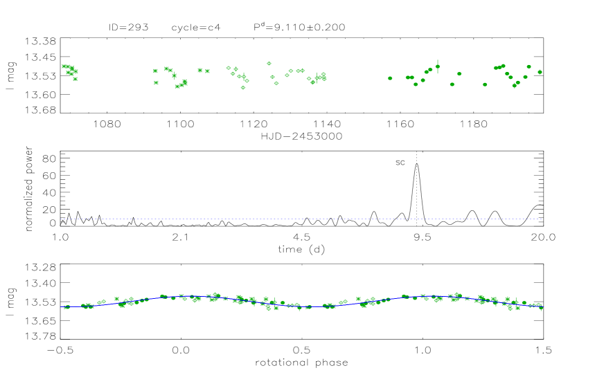
Figure 9: Results of periodogram analyses on the newly discovered periodic variable ID=293. Top panel: I-band time series data from cycle 4. Different symbols are used to better distinguish three different time intervals within the same observations season. Middle panels : Power spectra from Scargle analysis. The horizontal dashed line indicates the 99% confidence level, whereas the vertical dotted line marks the detected periodicity. Bottom panel phased light curve using the detected period.

As listed in Table 5, there is a large number of stars whose rotation period has been detected in all observing seasons including H02 data as well. The periodogram analysis performed on the whole 5-yr time series allows us to determine the rotation periods with accuracy better than 1%. Although the study of the long-term behaviour of our targets will be the prime subject of a subsequent paper, we show in Fig. 10 the light curves of one of these stars (ID=202), as an example. This example light curves show two interesting features. The first is that within the longest observing run (season 5), the light curve is very smooth and the shape has remained constant over about 5 months. This indicates that the size as well as the distribution of the spot which modulates the star light remain unchanged. This behaviour differs from what is observed in MS stars of similar rotation period, whose spot patterns are found to be stable over periods not longer than 1 to 2 months. However, we stress that this is the case for a limited number of stars in our sample, whereas there is a large number of stars whose rotation period, although detected in cycle 5 data, was not detected when the whole time series data was analysed. This is likely due to a rapid change of the spot pattern on these stars. Another feature is the change in amplitude, mean light level and migration of the light curve minimum from season to season. These latter variations may be related to the the presence of surface differential rotation (SDR) and ARGD.

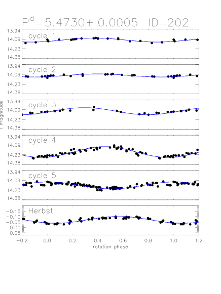
Figure 10: Example of light curves of one of our CTTS targets (ID=202) whose rotation period was detected in all our 5 observation season and in the Herbst et al. (2002) data as well.

As already mentioned, a part of our ONC field has been photometrically monitored since 1990 at Van Vleck Observatory by Herbst and collaborators (see, e.g., H00), in 1994 by S99, and in 1998-1999 by H02 at the MPG/ESO 2.2m telescope. Our analysis allowed us to identify a total of 148 periodic variables: 56 are the periodic stars newly discovered by us, whereas 92 were already known from the mentioned previous surveys (24 from Herbst and collaborators, 11 stars from S99, and 57 from both groups). We did not detect any periodicity in 18 stars, of which 2 were previously reported as periodic variables only by S99 (star 302 and 342) and 16 only by Herbst and collaborators (star 3, 4, 38, 39, 62, 69, 94, 114, 129, 152, 175, 208, 302, 327, 339, and 344). Actually, we note that previous surveys could detect the periodicity for 14 out of these 18 stars in only one observation season, hence their classification as a periodic variables can be considred tentative. Among the 92 stars with already known rotation period, there are 14 stars for which we detect a period different than that previously reported. However, we could understand the origin of the disagreement. For 5 stars (star 81, 96, 135, 181, 307), the rotation periods reported by either H02 or S99 are very different from ours. Looking at our periodograms of H02 averaged data we found a major power peak at the same period found in multiple seasons in the power spectra of our time series. However, such peaks have a power slightly smaller than the threshold (P_N=16.5) that they fixed and, therefore, they were not considered in the H02 sample. Indeed, this is an example of the advantage of multi-season with respect to single-season observations to obtain more reliable rotation periods.

For the stars 240, 254, 283, 296 we found a period that is almost doubled from the period reported by H02 or S99. This mismatch can be explained by considering that, at that time when these stars were observed, two major spots were located on opposite stellar hemispheres, giving rise to a flux modulation with half the period we found.

The disagreement to 4 stars (star 44, 285, 293, 303) is likely due to the beat phenomenon, ours or the H02 and S99 periods being beats of the true period. For star 274 we found in all seasons two different periods, one in common with H02 & S99 and another different. We adopted the latter, since it gives less scattered phased light curves.

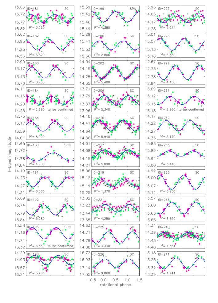
Figure 15: continued

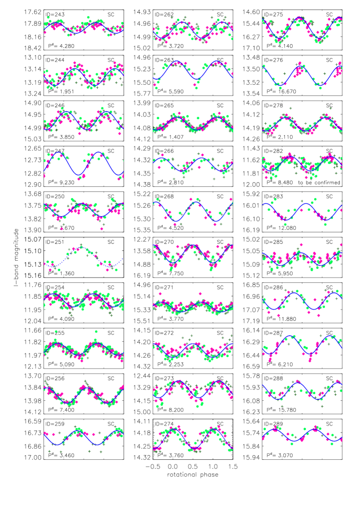
Figure 16: continued

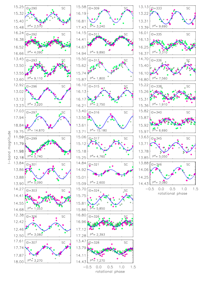
Figure 17: continued

Therefore, we can state that for 92 periodic stars, the results of our period search well conciliate with the results of previous studies. This point is very important, since it assures that we have been indeed collecting very precise photometric data as well as using a reliable period analysis technique. In addition to this we get confidence on our new detection of periodic variables and also confirmation of the previous findings. We have discovered 56 new periodic variables in our very small 10$\times$10 arc-min FOV and hence increased the total number of known periodic variables by almost 50%. However, we must note that 7 new periodic stars (identified with an apex ’a’ in Table 5) were detected as periodic for the first time by us and in only in one season. We need additional observations to confirm these periodicities, which will be considered at the present as tentative and will not be included in any subsequent analysis or statistics. For instance, the number of periodic stars whose period is detected in only one season ($\sim 5\%$) is similar to the total number of false detections expected in 5 observation seasons by fixing the FAP at 1%. We must consider with great caution also the 2 new periodic stars identified with an apex ’b’ in Table 5, since their period is very close to 1 day. Although, the same period was detected in multiple seasons, with high confidence level and giving smooth light curves, it may be an alias arising from the observation day-night duty cycle. They also will not be considered in the following analysis. The complete sample of light curves of our periodic variables are plotted in Figs. 13-17. In these figures we plot only one light curve per star, specifically the details of which has been listed in Table 5.

There are very few massive early spectral type stars in our FoV. Since such objects are saturated, almost all our program stars are low- to very low-mass objects and we treat them as TTS. In our FOV, till to date, 96 stars are found to show the H$\alpha$ line in emission and with very large EW, hence, these stars can be assumed as accreting CTTS. Whereas, the remaining 242 stars which lack the H$\alpha$ emission can be considered as WTTS. These numbers of CTTS and WTTS should be considered a preliminary estimate, and likely subjected to be changed in the future. In fact, as mentioned in Sect. 5., a few stars which were reported by previous studies as H$\alpha$ emission stars, are found by us with no emission, whereas 13 newly H$\alpha$ emitting stars have been identified by us. Thus, it appears that to identify all accreting CTTS using H$\alpha$ emission as a proxy, more extensive multi-year spectroscopic survey is needed. Moreover, we note that a few stars (like star 16, 41, 297 and 309) show an I-band light curve amplitude larger than 0.5 mag, although we have not detected H$\alpha$ emission. Such large amplitude most likely arises from the presence of both hot spots and variable extinction by the circum-stellar disk. Keeping these numbers distribution of WTTS and CTTS, our period search shows that about 72% of CTTS are periodic variables. Whereas, the percentage of periodic WTTS is about 32%. Our findind is contrary to Lamm et al. (2004), whose results on photometric monitoring of NGC2264 reveal that 85% WTTS and 15% CTTS are periodic variables.

From our study it appears that the detection of periodic signal related to rotation is easier in CTTS than in WTTS. This is surprising in the sense that, as mentioned previously, it is believed that the variability of CTTS is dominated by non-periodic phenomena, which should often prevent the detection of any periodic signal coming from the rotation (Herbst et al. 1994; Lamm et al. 2004). From the present study, it appears that the CTTS of ONC have patterns of surface inhomogeneities which give rise to the flux variations more stable than in WTTS and much more than in MS stars of similar period (see Fig. 10 as one example of stable CTTS light curve). The increased ability to detect rotation periods in CTTS may be due to the large amplitude of light modulation, a characteristic of CTTS. That compensates to some extent the presence of ”noisy” non-periodic phenomena, allowing the periodogram analysis to correctly identify the rotation period. The other possibility is that the number of CTTS identified from various H$\alpha$ emission surveys has been underestimated, and actual number of H$\alpha$ emitting CTTS are larger than the total number of 96 what we used for the calculation.

As we mentioned earlier, we have divided our entire FOV in three different regions and the number of spatial distribution of total as well as periodic variables are as follows. There are 59 stars residing in bright nebular region and designated as SNB, 98 stars are in partially nebular region (SPN), 189 are outside the nebula (SC). We could determine the rotation period of 27% (16/59) stars inside the nebula, of 33% (33/98) partially in the nebula, and of 52% (99/189) outside the nebula. As expected, the detection of periodic variables outside nebulosity, where the background light contribution is minimum and the photometric accuracy better, is much higher than inside nebulosity. Another possibility could be the presence of a large number of intermediate mass stars, inside the nebula, which are known for their irregular photometric behaviour. Finally, it was also found from previous studies that low-mass stars inside the Trapezium cluster are relatively younger (Hillenbrand 1997). Hence, it is quite possible that the youthness of these objects make their variability rather irregular.

The part of our FOV is very much affected by the presence of strong HII nebular emission and, hence, the background contribution is very high. In addition to this as mentioned earlier the distribution of the stellar mass as well as age are not uniform in this region, therefore, we attempted to get some information about the spatial distribution of periodic variables. In Fig. 11 we plot the spatial distribution of periodic variables over the FoV. The unexpected result what we find is that the detection frequency of the rotation period, i.e. number of seasons on which any object has been identified as periodic, is indistinguishable from inside to outside of the nebula. This result is surprising because the fact that inside the nebula, the observed magnitudes of stars are subjected to the lower photometric precision, objects are relatively massive and their age relative to the mean cluster age is less.

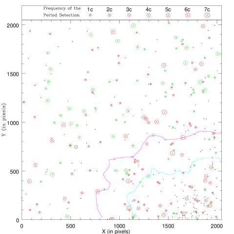
Figure 11: The spatial distribution of periodic variables. Open circle represent the periodic variable detected from our long-term monitoring program. Whereas the detection frequency is represented by size of the open circle, i.e. the largest circle correspond to the periodic variables, detected in all cycles including the previous surveys by Herbst et al. (2002) and Stassun et al. (1999). The green color represent the CTTS stars identified from H_α  emission and the red color represent WTTS and/or other unclassified stars found to be periodic.

5.4 Scarcity of short period variables

During cycles 4 and 5, we dedicated a number of nights to search for very fast rotating periodic variables. In order to make our time series data sensitive to very short-term flux modulations down to about 0.1 days, we monitored the ONC field over several full nights. Again, the data collected within one hour were combined and used as one single data point while doing time series analysis. These more numerous data collected within the same night allowed us to very accurately identify 22 periodic variables with period shorter than about two days, 5 of which were newly identified by us. We could also identify 2 new variables having periods very close to one day. These short period variables are reported in this paper because they have been detected in multiple seasons with high confidence level. However, their period need to be confirmed since they may be alias arising from the observation day-night duty cycle. The scarcity of very fast rotators (P$<$0.9d) in the magnitude range (12$<$I$<$17) explored by our survey supports the S99 finding on short-period variables. He first noticed that the ultra fast rotators that have been found in the Pleiades or in other older clusters are quite absent in the ONC, at least in the 12$<$I$<$17 magnitude range. This finding is quite expected for the low-mass stars of 1 Myr, whose break-up velocity is close to 0.5 days. However, here we like to emphasize that the fastest rotating stars identified by us in our FOV show a period about two times longer than S99. In contrast, after a few Myrs, like in NGC 2264, the number of rotators faster than 0.4 days increases rapidly. A very deep photometric monitoring campaign recently carried out by Rodriguez-Ledesma et al. (2008) in the ONC, shows the presence of very fast rotators (P$>$0.5d) among Very Low Mass Stars (VLM) and sub-stellar objects (BDs). These very fast rotating VLM and BDs probably possess different dynamo mechanism, operating in this mass regime and producing magnetic fields of different strength and topology as well (Herbst et al. 2006).

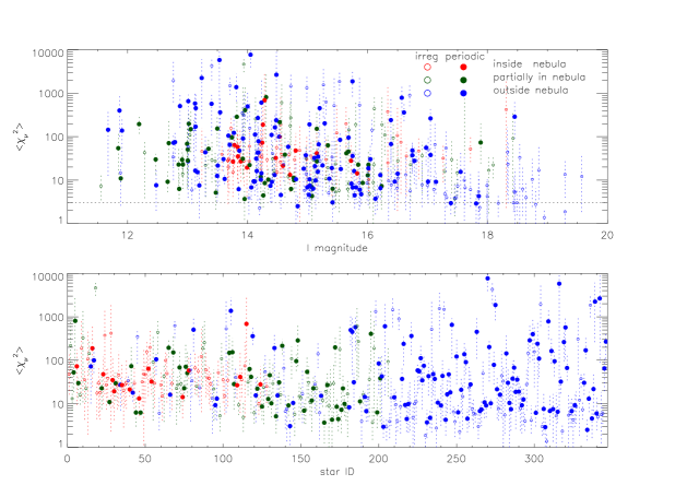
Figure 12: Top panel: Distribution of reduced chi-squares vs. I magnitude. Filled and open symbols are used to distinguish periodic from non periodic variables, whereas different color indicate the star’s position with respect to the nebula. Bottom panel: reduced chi-squares vs. internal ID number.

5.5 Non-periodic targets

We never detected evidence of periodic variability in 198 out of 346 stars. We have computed for each season the reduced chi-square ($\chi^{2}_{\nu}$) with respect to the seasonal median light level in order to quantify their level of variability. The $\chi^{2}_{\nu}$ of each star is found to vary from season to season. Their mean values vs. the median I magnitude (top panel) and vs. our internal ID number (bottom panel) are plotted in Fig. 12. The dashed vertical bars connect the minimum and maximum $\chi^{2}_{\nu}$ values ever observed. The red, green and blue colors indicate the target position with respect to the nebula (inside, partially inside and outside, respectively). Filled and open bullets represent periodic and non periodic variables, respectively.

Except the stars 230 and 308, which are the least variable in our sample, all non periodic targets can be classified as variable, having $\chi^{2}_{\nu}>3$ in at least one season. This is not a surprising finding since all targets are very young stars. They host numerous phenomena which induce variability in the optical as well as in other bands. Interestingly, the $\chi^{2}_{\nu}$ show a spatial dependence: their values monotonically decrease from inside to outside the nebula. This effect does not depend on the star’s brightness, as shown in the top panel of Fig. 12, but more likely on mass and age. As mentioned, a previous study (Hillenbrand 1997) shows a concentration of intermediate-mass stars inside the nebula, which are characterized by very irregular and large-amplitude variability. It is also quite possible that stars inside nebula are younger and, therefore, being more active give rise to a larger-amplitude variability.

6 Discussion and plan for near future

The luminosity spread in the color-magnitude diagram for stars having similar color, and hence mass, has been generally associated with the age spread and found to be an effective tool to explore the star formation history in young clusters (Hillenbrand 1997; Palla & Stahler 2000; Hartman 2001). However, limited photometric measurement accuracy, intrinsic variability and effect of binarity in the magnitudes can mask the signatures of the initial age spread. The use of the median magnitude from our long-term photometric monitoring of the ONC stars has allowed us to construct a CMD much more accurate than in previous studies, mostly based on snapshot observation, and, hence, has allowed us to better asses the presence/absence of any age spread in the ONC. It is quite apparent in the CMD of Fig. 8 that, after reddening correction, both WTTS and CTTS indeed show a spread in the magnitude at any color, which possibly points toward the presence of an age spread. However, we can not draw a very firm conclusion on this because of the small size of our sample and possible effects from unrecognized binaries as well as uncertain extinction correction. The presence/absence of spread in age of young stars has been subject of exploration over the last decade and contradictory claims have been made (Hartman 2001; Burningham et al. 2005; Jeffries 2007; Hillenbrand et al. 2008 and references their in). In near future, we expect to make further progress in our study on this subject by enlarging the size of our sample, identifying the binaries in our FOV as well as by a better measurement of the intra-cluster extinction correction.

Our multi-epoch observations have allowed us to identify in a very small FOV a large number periodic variables (an additional 50%). These newly identified periodic variables were unidentified mostly by previous surveys carried out over a single observing season. If we exclude massive stars or stars highly affected by nebulosity, then we found about 44% of stars in our FoV to be periodic. This is indeed a great gain with respect to previous surveys of S99 and H02 who discovered periodic variability only in 11% and 26%, respectively, of stars in our same FOV. Here we must keep in mind that the S99 and H00 surveys were carried out with much smaller aperture telescopes, hence on a smaller sample of brighter stars. We could obtain agreement with previously determined periods in $\sim$70% of stars, could explain the disagreement for 16% of periodic stars, whereas did not detect periodicity in the remaining 14% stars common in all these surveys. Our finding, and the results of other ongoing multi-year surveys (e.g. H00) as well, pose a strong warning about the completeness of the periodic variables discovered in young open clusters from single observing run, which is the most common case. If we extend our finding to other star forming regions photometrically monitored in only one season, we expect that the total number of periodic variables is highly underestimated. Therefore, when deriving any conclusion about the distribution of rotation period and its implication to angular momentum evolution, the sample incompleteness must be seriously taken into account.

Our monitoring program together with two previous surveys has yielded 148 periodic variables in a sample of 346 stars detected in our FOV. Except few stars, which show no definite variability, all the other stars were found to be variables, although with no systematic variations, i.e. irregular variables. It would be interesting to know what makes some stars periodic and others non-periodic. Is the undetected periodicity due to unfavourable inclination of the rotation axis, which does not allow the spot pattern visibility to be modulated? Or, is a very unstable spot pattern the major source of irregular behaviours of these non-periodic variables? In addition to these causes, sporadic accretion and extinction due to clumpy inner disk could be the source of irregular variation in the stars classified as a CTTS. We will be addressing all these questions in our forthcoming papers.

7 Conclusions

Five consecutive years of observation of a 10$\times$10 arc-minutes region of the ONC, using moderate size telescopes has allowed us to find several interesting results. We summarize our results below:

• We identified 13 new stars with moderate to strong H$\alpha$ emission, whereas, we did not detect emission in 7 stars, which were reported in the literature as strong H$\alpha$ emitters.

• The median multi-band magnitudes obtained from the long-term time series data have allowed us to put stellar members on HR diagrams more accurately than the previous studies. From the comparison with theoretical isochrones, it appears that the age of ONC is 1-2 Myr with a noticeable spread in the age.

• Our multi-year monitoring has allowed us to detect 56 new periodic variables, which increases by 50% the number of known periodic variables in the ONC region under study.

• From a comparison with previously know periodic variables we found matching periods for 70% variables. We find disagreement for 16% which can be explained either by period doubling or aliasing. To remaining 14% stars no period variation was detected.

• We also find the absence of stars with period shorter than 0.9 days in the 1 Myr old, brights members ( 12$<$I$<$17 mag) of the ONC.

• Despite very high background emission, a large number of periodic variables have been identified inside the nebula. These stars display a higher level of variability as for as reduced chi-square ($\chi^{2}_{\nu}$) is concern.

• Our study reveals that about 72% of CTTS in our FOV are periodic, whereas, percentage of periodic WTTS is just 32%. This indicate that inhomogeneity patterns on the surface of CTTS of the ONC are much more stable than in WTTS.

• All but two stars in our small FOV are found to be variable, according to the chi-square criterion.

[x]—l—r—r—r—r—@ c—r—@ r—@ c—@ c—@ l—@ l—@ c—@ c—@ c—c—@  Result of the periodogram analysis of periodic variables of the ONC.
ID JW Power   P$\pm\Delta$P   $\chi^{2}_{\nu}$   $<\sigma>$   $\Delta$I   #   #   #   n1   n2   n3   Sky   Object Type   Neighbour  

  (d)     (mag)   (mag)   obs.   mean   dis.        
Continued.
ID JW Power   P$\pm\Delta$P   $\chi^{2}_{\nu}$   $<\sigma>$   $\Delta$I   #   #   #   n1   n2   n3   Sky   Object Type   Neighbour  
  (d)     (mag)   (mag)   obs.   means   dis.        

5 265 45.59 6.540 $\pm$ 0.100 73.17 0.041 0.34 230 61 2 c4 c3/c5/H new SPN C y
15 710 15.68 7.810 $\pm$ 0.180 106.99 0.231 1.43 76 25 2 c2 c1/H =S SC C -
16 349 50.41 9.250 $\pm$ 0.120 173.62 0.054 0.63 397 101 6 c5 c3/c4 new SNB - -
17 125 16.71 8.860 $\pm$ 0.150 86.95 0.010 0.11 74 21 2 c3 c1/c4 new SC C -
18 278 60.60 6.840 $\pm$ 0.060 4189.88 0.016 1.60 400 102 6 c5 all =H SPN C -
23^a 366 18.86 8.790 $\pm$ 0.230 36.30 0.026 0.16 97 29 1 c2 - =H SNB - -
27 437 31.38 2.341 $\pm$ 0.008 11.60 0.018 0.09 180 88 5 c5 H =H SNB C -
29 417 15.58 7.370 $\pm$ 0.100 7.64 0.035 0.08 75 21 1 c3 c1/H =H SNB C -
31 622 19.93 3.770 $\pm$ 0.150 52.29 0.032 0.26 365 105 4 c5 c1/H new SNB - -
34 81 25.05 4.400 $\pm$ 0.040 26.53 0.010 0.12 62 21 2 c4 c1/c2/c3/H =H SC W -
35 9213 21.64 12.220 $\pm$ 1.410 16.13 0.039 0.34 103 21 1 c1 c3 new SNB - y
40 317 16.33 8.080 $\pm$ 0.190 14.37 0.018 0.08 97 29 3 c5 c2 =H SNB - -
41^b 3084 79.72 1.005 $\pm$ 0.001 93.87 0.165 1.07 410 106 8 c5 c1/c2/c3/c5 new SPN - -
42 71 28.67 14.400 $\pm$ 2.400 16.90 0.013 0.11 103 21 1 c1 c4/c5/H new SC - -
44 291 30.76 8.450 $\pm$ 0.210 5.93 0.009 0.04 223 61 2 c2 c4 $\neq$H SPN - -
51 658 28.97 3.204 $\pm$ 0.004 121.67 0.090 0.45 238 61 3 c4 c2/c3/c5 new SNB - -
52 356 27.28 4.840 $\pm$ 0.260 45.21 0.008 0.08 103 21 1 c1 c3/c4/c5/H =H SNB - -
54^a - 15.30 9.460 $\pm$ 0.170 45.33 0.072 0.30 77 21 2 c3 - new SNB - -
57 77 80.10 1.501 $\pm$ 0.004 47.05 0.013 0.19 245 62 2 c3 all =HS SC W -
65 678 31.20 12.870 $\pm$ 0.240 120.88 0.073 0.45 203 93 3 c5 c4/H =H SNB W -
66 130 22.84 1.206 $\pm$ 0.002 12.60 0.027 0.10 417 107 5 c5 all =H SC - -
68 292 25.68 5.120 $\pm$ 0.070 31.56 0.019 0.18 97 29 3 c2 c1/c4/c5/H new SPN - -
75 275 80.36 0.950 $\pm$ 0.001 18.84 0.014 0.09 411 107 6 c5 c1/c2/c4/H =H SPN - -
78^b 516 51.65 1.023 $\pm$ 0.001 45.39 0.035 0.26 415 107 4 c5 c1 new SNB - -
81 123 37.80 9.610 $\pm$ 1.050 330.29 0.004 0.16 90 21 1 c1 all $\neq$S SC - -
88 323 54.49 11.370 $\pm$ 0.020 766.12 0.021 0.73 417 107 5 c5 c1/c2/c3 new SPN C -
95 152 23.55 4.520 $\pm$ 0.240 9.61 0.006 0.03 103 21 1 c1 all new SC - -
96 183 25.00 1.871 $\pm$ 0.005 9.05 0.007 0.03 103 21 1 c1 c3/c4/H $\neq$H SC - -
104 636 36.26 10.770 $\pm$ 1.320 133.92 0.012 0.22 101 21 1 c1 c2/c4/H =H SNB C y
105 192 36.08 8.930 $\pm$ 0.230 1090.97 0.008 0.51 97 29 2 c2 all =S SC C -
107 551 32.64 19.150 $\pm$ 4.190 24.69 0.010 0.09 103 21 1 c1 c5 new SNB - y
109 535 36.81 18.170 $\pm$ 3.780 33.88 0.014 0.15 103 21 1 c1 c5 new SNB - -
115 674 22.80 6.110 $\pm$ 0.070 139.90 0.014 0.30 62 20 2 c3 c1/c2/c4 new SNB - -
117 299 28.69 2.770 $\pm$ 0.010 45.08 0.025 0.15 245 62 3 c4 c1 =H SPN C -
118 3104 49.41 3.120 $\pm$ 0.020 55.95 0.033 0.28 97 29 2 c2 all =H SPN - -
121 70 45.74 1.497 $\pm$ 0.005 19.48 0.011 0.09 246 62 4 c4 c1/c2/H =H SC - -
122 250 30.21 2.740 $\pm$ 0.010 9.13 0.012 0.06 245 62 1 c4 all =H SPN - -
125^a 234 16.92 3.960 $\pm$ 0.040 7.01 0.016 0.05 97 29 2 c2 - new SPN - -
130 324 27.69 6.250 $\pm$ 0.440 43.88 0.016 0.18 103 21 2 c1 c4/c5 new SPN C -
131 254 21.10 3.500 $\pm$ 0.010 11.30 0.017 0.06 417 107 5 c5 c1/c2/H =H SPN - -
133 104 58.44 1.772 $\pm$ 0.004 161.70 0.015 0.26 417 107 5 c5 c3/c4/H =H SC C -
134 280 31.71 1.990 $\pm$ 0.010 10.55 0.008 0.04 96 29 2 c2 all =HS SPN - -
135 - 19.17 3.620 $\pm$ 0.140 4.83 0.031 0.11 103 21 1 c1 H $\neq$H SC - -
136 245 43.45 8.820 $\pm$ 0.190 43.95 0.006 0.09 245 62 2 c4 c2/c5 =S SPN C -
138 485 36.25 9.670 $\pm$ 0.270 205.72 0.013 0.29 97 29 2 c2 all =H SPN - -
142 220 52.08 2.330 $\pm$ 0.010 15.02 0.005 0.05 208 58 3 c4 c1/H =H SPN C -
145 168 34.51 0.912 $\pm$ 0.009 16.10 0.010 0.07 103 21 1 c1 c4/c5/H =H SC W -
147 243 24.49 10.150 $\pm$ 0.300 52.89 0.006 0.10 97 29 1 c2 all =S SPN C -
148 258 31.36 9.940 $\pm$ 1.130 76.22 0.006 0.11 103 21 1 c1 c4/c5/H =H SPN C -
154 683 17.75 11.430 $\pm$ 0.190 12.92 0.028 0.13 205 91 2 c5 c4/H =H SPN - y
158 573 55.73 4.750 $\pm$ 0.030 14.14 0.043 0.23 417 107 4 c5 c3 new SPN C -
163 117 37.58 9.010 $\pm$ 0.500 10.08 0.010 0.06 244 62 2 c4 c1 =H SC C -
165 281 29.75 3.150 $\pm$ 0.110 6.15 0.005 0.03 103 21 1 c1 c4/H =H SPN - -
166 290 31.16 3.080 $\pm$ 0.010 45.72 0.009 0.12 103 21 2 c1 c3 new SPN - -
167 283 35.35 7.390 $\pm$ 0.620 27.85 0.009 0.07 103 21 2 c1 c4/c5/H =H SPN - -
170 392 16.05 3.900 $\pm$ 0.020 3.07 0.015 0.04 416 107 5 c3 c5 new SPN C -
172 268 39.08 9.850 $\pm$ 0.140 69.50 0.016 0.15 417 107 4 c5 c1/c3/c4/H =H SPN C -
173 477 39.36 6.670 $\pm$ 0.110 10.25 0.007 0.04 245 62 3 c4 c1/c3 new SPN - -
174 415 16.75 2.060 $\pm$ 0.010 10.25 0.007 0.04 245 62 3 c2 c1 new SPN - -
178 427 24.86 4.500 $\pm$ 0.060 15.82 0.008 0.05 97 29 2 c2 c1 new SPN C -
181 144 27.78 3.960 $\pm$ 0.030 9.23 0.012 0.05 245 62 2 c4 c1/c3 $\neq$H SC - -
182 164 25.28 6.520 $\pm$ 0.080 643.74 0.018 0.41 77 21 2 c3 all =H SC - -
183 137 29.62 8.730 $\pm$ 0.870 1027.81 0.009 0.36 103 21 2 c1 all =H SC - y
184^a 272 45.55 2.980 $\pm$ 0.020 7.05 0.008 0.05 245 62 3 c4 - new SC C -
185 136 32.00 8.900 $\pm$ 0.900 1062.74 0.009 0.51 103 21 1 c1 all =H SC C y
188 418 25.56 4.900 $\pm$ 0.040 12.98 0.013 0.06 77 21 2 c3 all new SPN - -
191 188 37.52 6.560 $\pm$ 0.120 12.49 0.008 0.05 97 29 2 c2 all =HS SC - -
192 105 22.84 5.280 $\pm$ 0.080 15.20 0.009 0.07 97 29 2 c2 c1 new SC - -
195 672 32.09 6.530 $\pm$ 0.110 1538.41 0.009 0.83 103 21 1 c1 - =HS SPN C -
198 102 111.78 5.280 $\pm$ 0.040 1369.67 0.016 0.76 417 107 7 c5 c3/c4 new SC C -
199 486 25.52 4.380 $\pm$ 0.050 5.72 0.010 0.05 97 29 1 c2 c1/c3 new SPN W -
200 149 20.15 2.806 $\pm$ 0.003 44.96 0.014 0.14 77 21 2 c3 H =S SC C -
201 704 28.59 6.790 $\pm$ 0.030 34.58 0.026 0.16 243 62 5 c4 c1/H new SPN - y
202 211 100.77 5.480 $\pm$ 0.050 129.97 0.005 0.15 245 62 1 c4 all =HS SC C -
204 334 41.31 5.340 $\pm$ 0.070 37.93 0.009 0.10 245 62 2 c4 c1 =S SC C -
216 422 142.43 5.940 $\pm$ 0.050 330.26 0.012 0.30 417 107 5 c5 c1/c3/c4 =S SC C -
217 591 44.60 5.090 $\pm$ 0.030 9.42 0.014 0.06 417 107 9 c5 c1 new SC - -
219 148 30.60 1.370 $\pm$ 0.010 18.31 0.010 0.07 245 62 1 c4 c2/c3/c5/H =HS SC C -
221 502 31.09 4.250 $\pm$ 0.010 206.77 0.008 0.19 245 62 3 c4 c1 new SC - -
225 138 40.46 4.340 $\pm$ 0.210 70.62 0.008 0.12 103 21 1 c1 c5/H =S SC C -
226 543 25.50 9.860 $\pm$ 0.190 75.04 0.029 0.23 77 21 2 c3 c1/c2/c4/c5 new SC - -
227 107 28.63 1.074 $\pm$ 0.005 48.85 0.009 0.12 245 62 3 c4 c1/c3 new SC C -
228 326 34.15 6.380 $\pm$ 0.120 17.71 0.010 0.08 97 29 2 c2 all =H SC - -
229 239 28.44 4.460 $\pm$ 0.210 60.67 0.004 0.10 76 18 1 c1 c3/c4/c5/H =HS SC C -
231^a 446 17.18 2.860 $\pm$ 0.090 3.15 0.012 0.03 103 21 1 c1 - new SC - -
232 222 25.53 5.170 $\pm$ 0.070 18.00 0.009 0.08 97 29 2 c2 all =HS SC C -
233 318 24.80 3.410 $\pm$ 0.030 5.96 0.010 0.04 103 21 1 c1 c3/c4/H =H SC - -
236 311 41.23 6.230 $\pm$ 0.440 65.69 0.006 0.13 103 21 2 c1 all =HS SC - -
238 76 60.99 6.350 $\pm$ 0.110 10.12 0.012 0.06 245 62 2 c4 all =H SC - -
240 120 20.10 1.551 $\pm$ 0.003 2.88 0.012 0.04 417 107 5 c5 c4 $\neq$S SC C -
241 158 18.81 1.941 $\pm$ 0.007 49.35 0.006 0.09 60 21 2 c3 all =S SC - -
243 - 25.08 4.280 $\pm$ 0.060 2.81 0.087 0.19 245 62 2 c4 c1/c4/c5 new SC - -
244 576 57.83 1.951 $\pm$ 0.009 9.61 0.010 0.06 243 62 3 c4 c2/c5/H =H SC C -
246 155 50.63 3.850 $\pm$ 0.040 8.50 0.010 0.05 245 62 3 c4 c1/c3/c4/c5 new SC C -
247 252 22.89 9.230 $\pm$ 0.930 115.14 0.005 0.14 80 21 1 c1 H new SC C y
250 135 50.30 3.670 $\pm$ 0.030 29.59 0.009 0.08 245 62 1 c4 c1/c5/H =H SC C -
251 181 26.76 1.360 $\pm$ 0.005 9.16 0.008 0.04 97 29 2 c2 all =HS SC C -
254 330 15.27 4.090 $\pm$ 0.060 10.99 0.031 0.09 386 105 1 c5 c4/H $\neq$H SC W -
255 232 72.27 5.090 $\pm$ 0.030 37.90 0.021 0.14 374 107 3 c5 c4/H =H SC W -
256 65 135.50 7.400 $\pm$ 0.080 79.32 0.013 0.17 366 101 5 c5 all =S SC W -
259 3130 23.02 3.460 $\pm$ 0.030 39.20 0.017 0.21 97 29 1 c2 all =H SC C -
262 218 30.82 3.720 $\pm$ 0.020 3.84 0.010 0.04 245 62 1 c4 all new SC - -
263 379 25.35 5.590 $\pm$ 0.060 1032.75 0.008 0.37 77 21 1 c3 all =H SC C -
265 428 67.20 1.407 $\pm$ 0.003 6.67 0.011 0.04 417 107 5 c5 c3/c4 new SC - -
266 556 16.18 2.810 $\pm$ 0.020 9.06 0.005 0.03 97 29 1 c2 c1/c4 new SC C -
268 577 20.99 4.520 $\pm$ 0.040 13.73 0.014 0.06 77 21 2 c3 c1/c2/c4 new SC C -
270 381 65.54 7.750 $\pm$ 0.080 8992.91 0.016 1.76 320 81 5 c5 c4/H =H SC C -
271 632 31.86 3.770 $\pm$ 0.010 35.57 0.034 0.13 413 106 10 c5 c1/c4/H =H SC C -
272 628 40.58 2.253 $\pm$ 0.002 11.11 0.008 0.06 245 62 4 c4 c3/H =HS SC C -
273 647 95.82 8.200 $\pm$ 0.800 4771.02 0.018 1.08 314 80 6 c5 all new SC C -
274 174 80.92 3.760 $\pm$ 0.030 66.39 0.007 0.11 245 62 5 c4 all $\neq$HS SC C -
275 571 80.32 4.140 $\pm$ 0.050 2997.36 0.014 1.30 245 62 3 c4 all new SC C -
276 91 36.26 16.670 $\pm$ 3.170 5.46 0.005 0.03 103 21 3 c1 c5/H =H SC C -
278 416 80.91 2.110 $\pm$ 0.010 22.53 0.009 0.07 245 62 4 c4 all =S SC - -
282^a 421 32.10 8.480 $\pm$ 0.100 41.38 0.029 0.20 265 101 3 c5 - new SC C -
283 3134 24.21 12.080 $\pm$ 1.670 15.20 0.015 0.11 103 21 1 c1 c2/c3/c4 $\neq$HS SC - -
285 517 20.44 5.950 $\pm$ 0.020 3.16 0.009 0.03 245 62 1 c4 c1 $\neq$S SC - -
286 5147 19.47 11.880 $\pm$ 0.280 40.71 0.018 0.14 77 21 2 c3 c1/c2/c4 new SC C -
287 633 30.60 6.210 $\pm$ 0.440 27.03 0.016 0.20 103 21 1 c1 c2/c5 new SC - -
288^a 96 22.49 15.780 $\pm$ 0.740 37.07 0.014 0.19 97 29 1 c2 - new SC C -
289 200 28.21 3.070 $\pm$ 0.100 38.40 0.009 0.09 103 21 1 c1 all =H SC C -
290 294 16.58 2.57 $\pm$ 0.070 43.74 0.007 0.09 97 29 1 c2 c1/c4/H =H SC C -
292 3138 24.49 4.090 $\pm$ 0.020 11.74 0.033 0.11 416 107 6 c5 all =H SC - -
293 159 73.41 9.110 $\pm$ 0.200 10.99 0.012 0.07 245 62 3 c4 c3/c5/H $\neq$H SC - -
296 673 46.42 3.220 $\pm$ 0.110 311.01 0.004 0.15 101 21 2 c1 c2/c4/c5/H $\neq$H SC C -
297 - 37.06 14.870 $\pm$ 2.530 1070.23 0.100 1.37 103 21 3 c1 all =H SC - -
299 165 94.85 5.740 $\pm$ 0.040 98.42 0.027 0.26 281 97 1 c5 c4/H =H SC C -
301 380 20.30 5.090 $\pm$ 0.250 12.48 0.004 0.03 103 21 2 c1 c3/c4/H =H SC C -
303 101 36.25 1.053 $\pm$ 0.004 102.95 0.008 0.15 245 62 4 c4 c3/c5 $\neq$S SC C -
306 375 23.34 3.060 $\pm$ 0.100 18.78 0.005 0.04 68 15 1 c1 c4 new SC - -
307 - 29.83 3.270 $\pm$ 0.120 4.91 0.038 0.14 103 21 1 c1 c4/c5/H $\neq$H SC - -
309 228 25.49 3.240 $\pm$ 0.020 769.84 0.045 1.01 77 21 3 c3 all =H SC - -
311 565 152.00 9.890 $\pm$ 0.140 292.73 0.015 0.26 416 107 10 c5 all new SC - -
313 649 36.03 1.800 $\pm$ 0.009 102.33 0.007 0.15 97 29 2 c2 all =H SC C -
315 227 30.72 2.750 $\pm$ 0.020 8.87 0.010 0.06 97 29 2 c2 c1 new SC - -
316 728 18.90 15.180 $\pm$ 2.970 119.24 0.008 0.15 51 15 1 c1 c5 =H SC C -
317 94 20.27 4.760 $\pm$ 0.040 13.17 0.015 0.08 77 21 3 c3 all =H SC C -
321 447 34.70 2.600 $\pm$ 0.070 41.10 0.006 0.06 103 21 2 c1 c3/H =S SC C -
324 186 17.81 5.850 $\pm$ 0.100 15.85 0.012 0.08 97 29 1 c2 all =HS SC C -
326 5159 30.26 2.393 $\pm$ 0.008 10.34 0.040 0.13 417 107 6 c5 c1/c4 new SC C -
328 498 62.41 7.270 $\pm$ 0.070 217.19 0.017 0.22 417 107 6 c5 all =H SC - -
333 501 37.24 9.690 $\pm$ 1.070 137.85 0.005 0.14 103 21 5 c1 all new SC C -
335 682 33.73 3.310 $\pm$ 0.010 13.12 0.020 0.13 282 70 5 c5 c1/c3/c4/H new SC - -
336 449 45.21 7.560 $\pm$ 0.140 1980.86 0.014 0.85 174 43 3 c4 c1 new SC C -
338 100 18.00 1.910 $\pm$ 0.030 4.79 0.013 0.04 246 62 4 c4 c5 $\sim$H SC - -
340 216 25.76 6.690 $\pm$ 0.110 2.42 0.014 0.04 244 62 2 c4 c2/c3/H new SC - -
345 639 65.53 5.050 $\pm$ 0.080 33.59 0.015 0.08 72 21 1 c4 all =HS SC - -
346 284 36.68 3.080 $\pm$ 0.100 292.15 0.006 0.28 101 20 1 c1 c2/c5/H =HS SC C -
a: The rotation period was detected in only one season and, although with a FAP $<$ 1%, it needs to be confirmed by future observations.
b: The rotation period, although detected in multiple seasons and with a FAP $<$ 1%, may be a beat period, being very close to the window function main peak.

References

- Anupama et al. (1994) Anupama G. C., Kembhavi A. K., Prabhu T. P., Singh K. P., Bhat P. N., 1994, A&AS, 103, 315
- Attridge & Herbst (1992) Attridge J. M., Herbst W., 1992, ApJ, 398, L61
- Bailer-Jones & Mundt (2001) Bailer-Jones C. A. L., Mundt R., 2001, A&A, 367, 218
- Bertout (2000) Bertout C., 2000, A&A, 363, 984
- Bibo & The (1991) Bibo E. A., The P. S., 1991, A&AS, 89, 319
- Bonnell & Bastien (1992) Bonnell I., Bastien P., 1992, ApJ, 401, L31
- Bouvier et al. (2007) Bouvier J., Alencar S. H. P., Harries T. J., Johns-Krull C. M., Romanova M. M., 2007, prpl.conf, 479
- Brown et al. (1996) Brown, Alexander, Deeney, Bryan D., Ayres, Thomas R., Veale, Anthony, Bennett, & Philip D., 1996, ApJS, 107, 263
- Burningham et al. (2005) Burningham B., Naylor T., Littlefair S. P., Jeffries R. D., 2005, MNRAS, 363, 1389
- Budding (1977) Budding E., 1977, Ap&SS, 48, 207
- Calvet & Gullbring (1998) Calvet N., Gullbring E., 1998, ApJ, 509, 802
- Cargile, Stassun, & Mathieu (2008) Cargile P. A., Stassun K. G., Mathieu R. D., 2008, ApJ, 674, 329
- Carpenter, Hillenbrand, & Skrutskie (2001) Carpenter J. M., Hillenbrand L. A., Skrutskie M. F., 2001, AJ, 121, 3160
- Chabrier Küker (2006) Chabrier G., Küker M., 2006, A&A, 446, 1027
- Choi & Herbst (1996) Choi P. I., Herbst W., 1996, AJ, 111, 283
- Cieza & Baliber (2007) Cieza L., Baliber N., 2007, ApJ, 671, 605
- Cohen, Herbst, & Williams (2004) Cohen R. E., Herbst W., Williams E. C., 2004, AJ, 127, 1602
- Cutri et al. (2003) Cutri R. M., et al., 2003, tmc..book,
- Distefano et al. (2007) Distefano E., et al., 2007, EAS, 25, 165
- Donati et al. (2008) Donati J.-F., et al., 2008, MNRAS, 390, 545
- Dorren (1987) Dorren J. D., 1987, ApJ, 320, 756
- Dullemond et al. (2003) Dullemond C. P., van den Ancker M. E., Acke B., van Boekel R., 2003, ApJ, 594, L47
- Duvert et al. (2000) Duvert G., Guilloteau S., Ménard F., Simon M., Dutrey A., 2000, A&A, 355, 165
- Eaton, Herbst, & Hillenbrand (1995) Eaton N. L., Herbst W., Hillenbrand L. A., 1995, AJ, 110, 1735
- Everett & Howell (2001) Everett M. E., Howell S. B., 2001, PASP, 113, 1428
- Fűrész et al. (2008) Fűrész G., Hartmann L. W., Megeath S. T., Szentgyorgyi A. H., Hamden E. T., 2008, ApJ, 676, 1109
- Flaccomio et al. (2003) Flaccomio E., Damiani F., Micela G., Sciortino S., Harnden F. R., Jr., Murray S. S., Wolk S. J., 2003, ApJ, 582, 382
- Getman et al. (2005) Getman K. V., et al., 2005, ApJS, 160, 319
- Gilliland & Brown (1988) Gilliland R. L., Brown T. M., 1988, PASP, 100, 754
- Grady et al. (2000) Grady C. A., Sitko M. L., Russell R. W., Lynch D. K., Hanner M. S., Perez M. R., Bjorkman K. S., de Winter D., 2000, prpl.conf, 613
- Grankin et al. (2007) Grankin K. N., Melnikov S. Y., Bouvier J., Herbst W., Shevchenko V. S., 2007, A&A, 461, 183
- Grinin, Rostopchina, & Shakhovskoi (1998) Grinin V. P., Rostopchina A. N., Shakhovskoi D. N., 1998, AstL, 24, 802
- Haro (1953) Haro G., 1953, ApJ, 117, 73
- Hartmann (2001) Hartmann L., 2001, AJ, 121, 1030
- Hartmann, Hinkle, & Calvet (2004) Hartmann L., Hinkle K., Calvet N., 2004, ApJ, 609, 906
- Herbig (2008) Herbig G. H., 2008, AJ, 135, 637
- Herbig & Terndrup (1986) Herbig G. H., Terndrup D. M., 1986, ApJ, 307, 609
- Herbst et al. (1994) Herbst W., Herbst D. K., Grossman E. J., Weinstein D., 1994, AJ, 108, 1906
- Herbst & Wittenmyer (1996) Herbst W., Wittenmyer R., 1996, AAS, 28, 1338
- Herbst et al. (2000) Herbst W., Rhode K. L., Hillenbrand L. A., Curran G., 2000, AJ, 119, 261
- Herbst et al. (2002) Herbst W., Bailer-Jones C. A. L., Mundt R., Meisenheimer K., Wackermann R., 2002, A&A, 396, 513
- Hillenbrand, Bauermeister, & White (2008) Hillenbrand L. A., Bauermeister A., White R. J., 2008, ASPC, 384, 200
- Hillenbrand (1997) Hillenbrand L. A., 1997, AJ, 113, 1733
- Hillenbrand & Hartmann (1998) Hillenbrand L. A., Hartmann L. W., 1998, ApJ, 492, 540
- Horne & Baliunas (1986) Horne J. H., Baliunas S. L., 1986, ApJ, 302, 757
- Howell (1989) Howell S. B., 1989, PASP, 101, 616
- Huff & Stahler (2006) Huff E. M., Stahler S. W., 2006, ApJ, 644, 355
- Irwin et al. (2007) Irwin J., et al., 2007, MNRAS, 380, 541
- Jardine, Gregory, & Donati (2008) Jardine M. M., Gregory S. G., Donati J.-F., 2008, MNRAS, 386, 688
- Jeffries (2007) Jeffries R. D., 2007, MNRAS, 381, 1169
- Johns-Krull (2007) Johns-Krull C. M., 2007, ApJ, 664, 975
- Kenyon & Hartmann (1995) Kenyon S. J., Hartmann L., 1995, ApJS, 101, 117
- Kovacs (1981) Kovacs G., 1981, Ap&SS, 78, 175
- Lada & Lada (2003) Lada C. J., Lada E. A., 2003, ARA&A, 41, 57
- Lamm et al. (2004) Lamm M. H., Bailer-Jones C. A. L., Mundt R., Herbst W., Scholz A., 2004, A&A, 417, 557
- Lamm et al. (2005) Lamm M. H., Mundt R., Bailer-Jones C. A. L., Herbst W., 2005, A&A, 430, 1005
- Landolt (1992) Landolt A. U., 1992, AJ, 104, 372
- Lodato & Clarke (2004) Lodato G., Clarke C. J., 2004, MNRAS, 353, 841
- Lucas & Roche (2000) Lucas P. W., Roche P. F., 2000, MNRAS, 314, 858
- Mahdavi & Kenyon (1998) Mahdavi A., Kenyon S. J., 1998, ApJ, 497, 342
- Mandel & Herbst (1991) Mandel G. N., Herbst W., 1991, ApJ, 383, L75
- Messina, Rodonò, & Cutispoto (2004) Messina S., Rodonò M., Cutispoto G., 2004, AN, 325, 660
- Medhi (2006) Medhi, Biman J., 2006, PhDT, 45M
- Natta et al. (1997) Natta A., Grinin V. P., Mannings V., Ungerechts H., 1997, ApJ, 491, 885
- O’dell (2001) O’dell C. R., 2001, ARA&A, 39, 99
- Palla et al. (2005) Palla F., Randich S., Flaccomio E., Pallavicini R., 2005, ApJ, 626, L49
- Palla & Stahler (2000) Palla F., Stahler S. W., 2000, ApJ, 540, 255
- Pontoppidan et al. (2007) Pontoppidan K. M., Dullemond C. P., Blake G. A., Boogert A. C. A., van Dishoeck E. F., Evans N. J., II, Kessler-Silacci J., Lahuis F., 2007, ApJ, 656, 980
- Preibisch et al. (2005) Preibisch T., et al., 2005, ApJS, 160, 401
- Rebull (2001) Rebull L. M., 2001, AJ, 121, 1676
- Rebull et al. (2006) Rebull L. M., Stauffer J. R., Megeath S. T., Hora J. L., Hartmann L., 2006, ApJ, 646, 297
- Rebull, Wolff, & Strom (2004) Rebull L. M., Wolff S. C., Strom S. E., 2004, AJ, 127, 1029
- Rodriguez-Ledesma (2008) YSC’15 Proceedings of Contributed Papers (eds. Choliy V. Ya., Ivashchenko G.), 2008, pp. 21-24
- Scargle (1982) Scargle J. D., 1982, ApJ, 263, 835
- Sicilia-Aguilar et al. (2005) Sicilia-Aguilar A., et al., 2005, AJ, 129, 363
- Siess, Dufour, & Forestini (2000) Siess L., Dufour E., Forestini M., 2000, A&A, 358, 593
- Skelly et al. (2008) Skelly M. B., Unruh Y. C., Cameron A. C., Barnes J. R., Donati J.-F., Lawson W. A., Carter B. D., 2008, MNRAS, 385, 708
- Stassun et al. (2004) Stassun K. G., Ardila D. R., Barsony M., Basri G., Mathieu R. D., 2004, AJ, 127, 3537
- Stassun et al. (1999) Stassun K. G., Mathieu R. D., Mazeh T., Vrba F. J., 1999, AJ, 117, 2941
- Stetson (1992) Stetson P. B., 1992, ASPC, 25, 297
- Stetson (1987) Stetson P. B., 1987, PASP, 99, 191
- Strassmeier (2002) Strassmeier K. G., 2002, AN, 323, 309
- Vorobyov & Basu (2005) Vorobyov E. I., Basu S., 2005, ApJ, 633, L137
- Wallace (1994) Wallace P. T., 1994, ASPC, 61, 481
- Waters & Waelkens (1998) Waters L. B. F. M., Waelkens C., 1998, ARA&A, 36, 233
- Wiramihardja et al. (1991) Wiramihardja S. D., Kogure T., Yoshida S., Nakano M., Ogura K., Iwata T., 1991, PASJ, 43, 27