How the result of a measurement of a component of the spin of a spin-1/2 particle can turn out to be 100 without using weak measurements

Abstract

We discuss two questions related to the concept of weak values as seen from the standard quantum-mechanics point of view. In the first part of the paper, we describe a scenario where unphysical results similar to those encountered in the study of weak values are obtained using a simple experimental setup that does not involve weak measurements. In the second part of the paper, we discuss the correct physical description, according to quantum mechanics, of what is being measured in a weak-value-type experiment.

I Introduction

The first part of the title of this paper (all but the last four words) is taken from the title of a paper written by Aharonov, Albert and Vaidman (AAV) over twenty years ago Aharonov . In that paper AAV introduced the concept of weak values. This concept immediately caused controversy Comments , but over the years it has proved to be a useful paradigm for considering questions related to quantum measurement and the foundations of quantum mechanics. For example, the observation of paradoxical values in a weak-value-type measurement has been linked to the violation of the Leggett-Garg inequality, which can be used to test realism LeggettGarg ; Williams ; Romito .

In the setup considered by AAV, a beam of spin-1/2 particles propagates through a non-uniform magnetic field in a Stern-Gerlach-type experiment, where the trajectory of a given particle is affected by the spin state of the particle. The modification from the original Stern-Gerlach experiment is that, in the path of its propagation, the beam encounters two regions in space with magnetic fields. The magnetic field gradient in the first region is designed such that it creates a tendency for particles whose $x$-component of the spin (which we denote by $S_{x}$) is positive to develop a finite component of the momentum in the positive $x$ direction and for particles whose $S_{x}$ is negative to develop a finite component of the momentum in the negative $x$ direction. After exiting this region in space, the beam enters a second region where a $z$-component in the momentum develops based on the $z$-component of the spin ($S_{z}$). Either one of these stages would constitute a measurement of the spin along some direction: by setting up a screen that the beam hits sufficiently far from the field-gradient region, the position where a given particle hits the screen serves as an indicator of the particle’s spin state. When combined, they create a situation where two non-commuting variables are being measured in succession. If (1) the first measurement stage is designed to be a weak measurement, (2) the particles in the beam are created in a certain initial state [e.g. close to being completely polarized along the positive $z$-axis] and (3) only those particles for which the second measurement produces a certain outcome [in this example, a negative $z$-component of the spin], then the average value of the spin’s $x$-component indicator can suggest values of this component of spin being much larger than 1/2, a situation that seems paradoxical.

A number of studies have already pointed out that since in the AAV setup two non-commuting variables are being measured in succession, quantum mechanics forbids treating them as independent measurements whose outcomes do not affect one another Comments . In this paper we start by presenting an example that demonstrates the role of interpretation in obtaining unphysical results in a weak-measurement-related setup. The setup is chosen to be very simple in order to remove any complications in the analysis related to the successive measurement of non-commuting variables. In the second part of the paper, we present the proper analysis (from the point of view of quantum mechanics) of the measurement results obtained in an AAV setup.

II Question 1: Unphysical results of the AAV type in an alternative setup

Let us consider the following situation: An experimenter purchases a device for measuring the $z$-component of a spin-1/2 particle. The device produces one of two readings, 0 or 1. The experimenter goes to the lab and calibrates the device. The calibration is done by preparing $10^{6}$ particles in the spin up state, measuring them one by one, and then doing the same for the spin down state. Let us say that the result of the calibration procedure is that for the spin up state the device shows the reading “1” in 50.25% of the experimental runs and the reading “0” in 49.75% of the runs. For the spin down state, the probabilities are reversed. Clearly, the reading of the measurement device is only weakly correlated with the spin state of the measured particle. The experimenter takes this fact into account and reaches the following conclusion: If I have a large number of identically prepared spin-1/2 particles and measure them using this device, I will obtain a probability for the reading “1”. Using the results of the calibration procedure, the expectation value of the spin $z$-component for the prepared state will be given by the formula:

$$\left\langle S_{z}\right\rangle=\left({\rm Prob_{1}}-0.5\right)\times 200.$$ (1)

If the probability of obtaining the outcome “1” is 0.5025, the above formula gives 1/2. If the probability of obtaining the outcome “1” is 0.4975, the above formula gives -1/2. It looks like the device is ready to be used. The experimenter now performs an experiment that involves, as its final step, a measurement of $S_{z}$. Surprisingly, the measurement device shows the reading “1” every time the experiment is repeated, leading the experimenter to conclude that the value of the spin is in fact 100. Thus one has a paradox.

The resolution of the paradox in the above story lies in the fact that the device was not a weak-measurement device as the experimenter assumed, but a strong-measurement device whose reading is perfectly correlated with the spin state of the measured particle. The only problem is that at some point before the measurement device was calibrated, its spin-sensing part was rotated from being parallel to the $z$-axis to an axis that makes an angle 89.7135 with the $z$-axis (note here that $\cos^{2}(89.7135/2)\approx 0.5025$). Not surprisingly, the calibration procedure produced the probabilities 0.5025 and 0.4975. In the “real” experiment, the spins were all aligned with the measurement axis of the device, and the reading “1” was observed in all the runs. The paradox is therefore resolved.

An unquestioning believer in quantum mechanics might say that the situation discussed in Ref. Aharonov has a large amount of overlap with the story presented above. In both cases a perfectly acceptable measurement is performed. The reason for obtaining a paradoxical measurement result is simply the wrong interpretation of what the measurement device is measuring and the resulting erroneous mapping from measurement outcomes to values of the measured quantity.

III Question 2: Correct explanation of results in an AAV setup

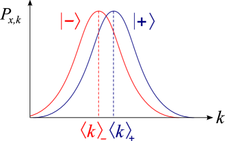
Figure 1: (color online) Schematic diagram of the probability distributions of the possible measurement outcomes of a weak measurement (labelled by the index $k$) for the two states of the measurement basis, $\left|+\right\rangle$ and $\left|-\right\rangle$.

We now turn to the question of the correct interpretation of the AAV experiment according to quantum mechanics. Instead of the original, Stern-Gerlach-type experiment analyzed by AAV, we formulate the problem slightly differently. We consider a spin-1/2 particle that is subjected to two separate measurements. As a first step, a weak measurement is performed in the basis $\left\{\left|+\right\rangle,\left|-\right\rangle\right\}$, where $\left|\pm\right\rangle=(\left|\uparrow\right\rangle\pm\left|\downarrow\right\rangle)/\sqrt{2}$ and the states $\left|\uparrow\right\rangle$ and $\left|\downarrow\right\rangle$ are the eigenstates of $\hat{S}_{z}$. This measurement can produce any one of a large number of possible outcomes, with probability distributions as shown in Fig. 1. This measurement constitutes a weak measurement of $\hat{S}_{x}$. As discussed in Ashhab , each possible outcome is associated with a measurement matrix $\hat{U}_{x,k}$, where the index $k$ represents the outcome that is observed in a given run of the experiment. If the outcome $k$ occurs with probability $P_{x,k}$ for the system’s maximally mixed state, i.e. when averaged over all possible initial states, and it provides measurement fidelity $F_{x,k}$ (in favor of the state $\left|+\right\rangle$), the measurement matrix $\hat{U}_{x,k}$ is given by

$$\hat{U}_{x,k} = \sqrt{P_{x,k}}\left\{\sqrt{1+F_{x,k}}\left|+\right\rangle\left\langle+\right|+\sqrt{1-F_{x,k}}\left|-\right\rangle\left\langle-\right|\right\}$$ (4)

$$= \frac{\sqrt{P_{x,k}}}{2}\left(\begin{array}[]{cc}\sqrt{1+F_{x,k}}+\sqrt{1-F_{x,k}}&\sqrt{1+F_{x,k}}-\sqrt{1-F_{x,k}}\\ \sqrt{1+F_{x,k}}-\sqrt{1-F_{x,k}}&\sqrt{1+F_{x,k}}+\sqrt{1-F_{x,k}}\\ \end{array}\right).$$

We shall use the convention where a measurement that favors the state $\left|-\right\rangle$ has a negative value of $F_{x,k}$ and $\hat{U}_{x,k}$ is given by the same expression as above. It is worth mentioning here that the overall, or average, fidelity of this measurement can be obtained by averaging over all possible initial states and all possible outcomes:

$$\left\langle F_{x}\right\rangle=\sum_{k}P_{x,k}\left|F_{x,k}\right|.$$ (5)

After the weak $x$-basis measurement, a strong measurement in the $\left\{\left|\uparrow\right\rangle,\left|\downarrow\right\rangle\right\}$ basis is performed. This strong measurement step can be described by two outcomes with corresponding measurement matrices

$$\hat{U}_{z,1} = \left|\uparrow\right\rangle\left\langle\uparrow\right|$$ (8)

$$= \left(\begin{array}[]{cc}1&0\\ 0&0\\ \end{array}\right)$$

$$\hat{U}_{z,2} = \left|\downarrow\right\rangle\left\langle\downarrow\right|$$ (11)

$$= \left(\begin{array}[]{cc}0&0\\ 0&1\\ \end{array}\right).$$

As mentioned above, paradoxes arise if one treats the $x$-basis and $z$-basis measurements as two separate measurements that provide complementary information. Instead, one should treat each pair of outcomes as a single combined-measurement outcome. The maximum amount of information in a given run of the experiment can be extracted as follows Ashhab : given that the outcome pair $\{k,l\}$ was observed, one can construct the combined-measurement matrix

$$\hat{U}_{{\rm Total},k,l}=\hat{U}_{z,l}\hat{U}_{x,k}.$$ (12)

From the matrices $\hat{U}_{{\rm Total},k,l}$ one can construct a so-called positive operator-valued measure (POVM) defined by the matrices $\hat{M}_{k,l}$:

$$\hat{M}_{k,l}=\hat{U}_{{\rm Total},k,l}^{\dagger}\hat{U}_{{\rm Total},k,l},$$ (13)

where the superscript $\dagger$ represents the transpose conjugate of a matrix. In particular,

$$\hat{M}_{k,1} = \frac{P_{x,k}}{2}\left(\begin{array}[]{cc}\left(\sqrt{1+F_{x,k}}+\sqrt{1-F_{x,k}}\right)^{2}&2F_{x,k}\\ 2F_{x,k}&\left(\sqrt{1+F_{x,k}}-\sqrt{1-F_{x,k}}\right)^{2}\\ \end{array}\right)$$

$$= P_{x,k}\left(1+\left|\psi_{k,1}\right\rangle\left\langle\psi_{k,1}\right|-\left|\overline{\psi}_{k,1}\right\rangle\left\langle\overline{\psi}_{k,1}\right|\right)$$

$$= 2P_{x,k}\left|\psi_{k,1}\right\rangle\left\langle\psi_{k,1}\right|$$ (17)

where

$$\left|\psi_{k,1}\right\rangle = \cos\frac{\theta_{k}}{2}\left|\uparrow\right\rangle+\sin\frac{\theta_{k}}{2}\left|\downarrow\right\rangle$$

$$\left|\overline{\psi}_{k,1}\right\rangle = \sin\frac{\theta_{k}}{2}\left|\uparrow\right\rangle-\cos\frac{\theta_{k}}{2}\left|\downarrow\right\rangle$$

$$\sin\theta_{k} = F_{x,k}.$$ (18)

Similarly one can find that

$$\hat{M}_{k,2} = 2P_{x,k}\left|\psi_{k,2}\right\rangle\left\langle\psi_{k,2}\right|$$

$$\left|\psi_{k,2}\right\rangle = \sin\frac{\theta_{k}}{2}\left|\uparrow\right\rangle+\cos\frac{\theta_{k}}{2}\left|\downarrow\right\rangle,$$ (19)

with $\theta_{k}$ given by the same expression as above.

As discussed in Ref. Ashhab , one can obtain the measurement basis and fidelity that correspond to the outcome defined by $\{k,l\}$ by diagonalizing the matrix $\hat{M}_{k,l}$. Since $\hat{M}_{k,l}$ is a hermitian matrix, its two eigenvalues ($m_{k,l,1}$ and $m_{k,l,2}$, with $m_{k,l,1}\geq m_{k,l,2}$) will be real and its two eigenstates ($\left|\psi_{k,l}\right\rangle$ and $\left|\overline{\psi}_{k,l}\right\rangle$) will be orthogonal quantum states that define a basis (the measurement basis). Note that because the second measurement in the problem considered here is a strong measurement, we always have $m_{k,l,2}=0$.

The different outcomes produce different measurement bases, thus this measurement cannot be thought of in the usual sense of measuring $S_{\bf n}$ with ${\bf n}$ being some fixed direction. Therefore, the measurement basis is determined stochastically for each (combined) measurement (note that after the strong $z$-basis measurement, the system always ends up in one of the states $\{\left|\uparrow\right\rangle,\left|\downarrow\right\rangle\}$, even though the combined-measurement basis can be different from the basis $\{\left|\uparrow\right\rangle,\left|\downarrow\right\rangle\}$). By analyzing all the measurement data, one can perform partial quantum state tomography and determine the $x$ and $z$-components in the initial state of the system (assuming of course that all copies are prepared in the same state, which can be pure or mixed). Note that in this setup no information about $S_{y}$ can be obtained from the measurement outcome.

We now ask whether information can be extracted from the $x$-basis and $z$-basis measurements separately, i.e. by disregarding the outcome of one of the two measurement steps. The answer is yes, provided care is taken in interpreting the results. Extracting an $x$-basis measurement from a given measurement outcome is straightforward. All one has to do is disregard the outcome of the $z$-basis measurement, since this measurement is performed after the $x$-basis measurement and cannot affect the outcome of the $x$-basis measurement. Therefore, by disregarding the outcome of the $z$-basis measurement, one obtains an $x$-basis measurement with overall fidelity $\left\langle F_{x}\right\rangle$. The situation is somewhat trickier if one wants to extract a $z$-basis measurement from the measurement outcome. One can disregard the outcome of the $x$-basis measurement, but one must take into account the fact that this measurement generally changes the state of the system before the $z$-basis measurement is performed. The effect of the $x$-basis measurement is to reduce the fidelity of the $z$-basis measurement. One can calculate this reduced fidelity as follows: Let us assume that the system starts in the initial state $\left|\uparrow\right\rangle$. After the $x$-basis measurement is performed and the outcome $k$ (with fidelity $F_{x,k}$) is observed, the state of the system is transformed into a new pure state $\left|\psi_{\rm int}\right\rangle$ with $\left|\left\langle\psi_{\rm int}\right|\hat{\sigma}_{x}\left|\psi_{\rm int}\right\rangle\right|=F_{x,k}$. Since

$$\left|\left\langle\psi_{\rm int}\right|\hat{\sigma}_{x}\left|\psi_{\rm int}\right\rangle\right|^{2}+\left|\left\langle\psi_{\rm int}\right|\hat{\sigma}_{y}\left|\psi_{\rm int}\right\rangle\right|^{2}+\left|\left\langle\psi_{\rm int}\right|\hat{\sigma}_{z}\left|\psi_{\rm int}\right\rangle\right|^{2}=\frac{1}{4}$$ (20)

for any pure state and here we have $\left|\left\langle\psi_{\rm int}\right|\hat{\sigma}_{y}\left|\psi_{\rm int}\right\rangle\right|=0$, we find that after the $x$-basis measurement $4\left|\left\langle\psi_{\rm int}\right|\hat{\sigma}_{z}\left|\psi_{\rm int}\right\rangle\right|$ is reduced from 1 to $\sqrt{1-F_{x,k}^{2}}$. If $F_{x,k}$ is independent of $k$, one obtains the relation (in this context, see e.g. Ref. Kurotani )

$$\left\langle F_{x}\right\rangle^{2}+\left\langle F_{z}\right\rangle^{2}=1.$$ (21)

We now take one final look at the AAV gedankenexperiment. We choose a specific form for the $x$-basis measurement, which is essentially the same one used by AAV

$$P_{x,k} = \frac{1}{\sqrt{2\pi k_{\rm rms}^{2}}}\exp\left\{-\frac{k^{2}}{2k_{\rm rms}^{2}}\right\}$$

$$F_{x,k} = \sqrt{\frac{\pi}{2}}\frac{\left\langle F_{x}\right\rangle}{k_{\rm rms}}k,$$ (22)

with $k$ running over all integers from $-\infty$ to $+\infty$ and $k_{\rm rms}$ assumed to be a large number. Note that the above expression violates the constraint that $F_{x,k}<1$. However, provided that $\left\langle F_{x}\right\rangle\ll 1$, the above expression can be treated as a good approximation of the realistic situation for all practical purposes. A simple calculation shows that in this case

$$\left\langle F_{z}\right\rangle = \sum_{k=-\infty}^{\infty}\sqrt{1-F_{x,k}^{2}}P_{x,k}$$ (23)

$$\approx 1-\frac{\pi\left\langle F_{x}\right\rangle^{2}}{4},$$

such that

$$\left\langle F_{x}\right\rangle^{2}+\left\langle F_{z}\right\rangle^{2}\approx 1-\frac{\pi-2}{2}\left\langle F_{x}\right\rangle^{2}.$$ (24)

If the measured system is prepared in one of the states $\left|\pm\right\rangle$, the average value of $k$ that is obtained in an ensemble of measurements (all with the same initial state) is

$$\left\langle k\right\rangle_{\left|\pm\right\rangle}=\pm\frac{\left\langle F_{x}\right\rangle k_{\rm rms}}{2}.$$ (25)

The small difference between $\left\langle k\right\rangle_{\left|+\right\rangle}$ and $\left\langle k\right\rangle_{\left|-\right\rangle}$ is the reason why the $x$-basis measurement qualifies as a weak measurement of $S_{x}$. We now consider the full measurement procedure. If one prepares the measured system in a state that is very close to $\left|\uparrow\right\rangle$, most $z$ basis measurements will produce the outcome $l=1$. Only a small fraction of the experimental runs will produce the outcome $l=2$. If the initial state deviates slightly from $\left|\uparrow\right\rangle$, i.e.

$$\left|\psi_{i}\right\rangle=\cos\frac{\alpha}{2}\left|\uparrow\right\rangle+\sin\frac{\alpha}{2}\left|\downarrow\right\rangle,$$ (26)

then outcomes with negative values of $k$ and $l=2$ will be suppressed the most (assuming $\alpha$ is positive), because these outcomes correspond to states that are orthogonal or almost orthogonal to the initial state (making their occurrence probabilities particularly small). One therefore finds that among the measurements that produced $l=2$, the average value of $k$ can be much larger than $\left\langle k\right\rangle_{\left|+\right\rangle}$ for properly chosen parameters. This situation leads to the AAV paradox.

IV Conclusion

In conclusion, we have presented explanations according to quantum mechanics of two questions that are relevant to discussions of weak values. First we presented an example that emphasizes the role of interpretation in obtaining unphysical results in an AAV setup. We have also presented the correct interpretation (according to quantum mechanics) of the measurement results obtained in an AAV setup. We believe that our discussion is useful for understanding the origin of the possible observation of unphysical values in a weak-value experimental setup.

This work was supported in part by the National Security Agency (NSA), the Laboratory for Physical Sciences (LPS), the Army Research Office (ARO) and the National Science Foundation (NSF) grant No. EIA-0130383.

References

- (1) Y. Aharonov, D. Z. Albert, and L. Vaidman, Phys. Rev. Lett. 60, 1351 (1988).
- (2) A. J. Leggett, Phys. Rev. Lett. 62, 2325 (1989); A. Peres, ibid 62, 2326 (1989); Y. Aharonov and L. Vaidman, ibid 62, 2327 (1989).
- (3) A. J. Leggett and A. Garg, Phys. Rev. Lett. 54, 857 (1985); A. J. Leggett, J. Phys. Condens. Matter 14, R415 (2002).
- (4) N. S. Williams and A. N. Jordan, Phys. Rev. Lett. 100, 026804 (2008).
- (5) For other studies on the subject, see e.g. A. Romito, Y. Gefen, and Y. M. Blanter, Phys. Rev. Lett. 100, 056801 (2008); V. Shpitalnik, Y. Gefen, and A. Romito, Phys. Rev. Lett. 101, 226802 (2008).
- (6) S. Ashhab, J. Q. You, and F. Nori, Phys. Rev. A 79, 032317 (2009); arXiv:0903.2319.
- (7) Y. Kurotani, T. Sagawa, and M. Ueda, Phys. Rev. A 76, 022325 (2007).