Long Range Free Bosonic Models in Block Decimation Notation: Applications and Entanglement

Abstract

We study the effect of long range particle exchange in bosonic arrangements. We show that by combining the solution of the Heisenberg equations of motion with matrix product state representation it is possible to investigate the dynamics as well as the ground state while including particle exchange beyond next-neighbours sites. These ideas are then applied to study the emergence of entanglement as a result of scattering in boson chains. We propose a scheme to generate highly entangled multi-particle states that exploits collision as a powerful entangling mechanism.

Experimental advancements in low temperature physics increasingly improve the control and handling of Bose Einstein condensates and other highly correlated states of matter where quantum mechanics phenomena emerge in their more elemental form. As a consequence, the gap between experiment and first principle analysis via clever numerical methodologies is continuously narrowing down. Powerful numerical methods as density matrix renormalization group and time evolving block decimation (TEBD) vidal1 allow to simulate systems of considerable complexity and size, but in most cases both methods are limited to short range interactions among neighbour elements. Therefore, developing practical methods to carry out numerics including interactions at long scope is very important, as such mechanisms are integral elements of many physical systems, e.g., when Coulomb forces are involved. As it is well known, a lot of theoretical and experimental work has been done seeking to understand quantum systems and intensive research is currently carried out in many diverse fields ResBos ; Reslen ; Plenio ; Rey ; Cirac . In this way motivated, here we explore practical alternatives for the study of quantum systems. We complement this discussion by using our findings to explore the quantum behaviour of 1D boson arrangements. We also focus on how much entanglement is generated after bosons collide in a chain. Although it has been shown that interacting wave packets get entangled after collision Law ; Jacksh , most of the studies on this subject focus on systems made of just two particles, hence applications in many-body configurations constitute an important investigation.

Let us consider a 1D arrangement of $N$ sites in which boson exchange can take place at all scales. The Hamiltonian is given by

$$\hat{H}=\sum_{k=1}^{N}\sum_{l=k}^{N}{R_{k,l}\hat{a}^{\dagger}_{k}\hat{a}_{l}+h.c}$$ (1)

$R_{k,l}$ determines the intensity of the hopping between sites $k$ and $l$ while the creation and annihilation operators obey the usual commuting rules $[\hat{a}_{l},\hat{a}^{\dagger}_{k}]=\delta_{k}^{l}$ and $[\hat{a}_{k},\hat{a}_{l}]=[\hat{a}^{\dagger}_{k},\hat{a}^{\dagger}_{l}]=0$. Hamiltonian (1) is integrable (quadratic) and the Heisenberg equations of motion for the creation operators yield a complete set of differential equations of the form

$$\frac{d\hat{\alpha}_{k}}{dt}=-i\sum_{l=0}^{N}R_{k,l}\hat{\alpha}_{l}\Rightarrow\frac{d\mbox{ \boldmath$\hat{\alpha}$ }}{dt}=-i\hat{R}\mbox{\boldmath$\hat{\alpha}$},$$ (2)

subject to the initial condition $\hat{\alpha}_{k}(t=0)=\hat{a}_{k}^{\dagger}$. We recall $\hat{\alpha}_{k}=e^{-it\hat{H}}\hat{a}^{\dagger}_{k}e^{it\hat{H}}$. The time dependent state ket is given by $|\psi(t)\rangle=\prod_{k}^{N}\hat{\alpha}_{k}^{n_{k}}|0\rangle/\sqrt{\prod_{j}^{N}n_{j}!}$, in such a way that the $n_{k}$’s determine the initial configuration of bosons. Similarly, the ground state can be obtained by diagonalizing Hamiltonian (1). Such ground state can be written as

$$|G\rangle=\left(\sum_{k=0}^{N}c_{k}\hat{a}^{\dagger}_{k}\right)^{M}|0\rangle,$$ (3)

where coefficients $c_{k}$ are the components of the ground eigenvector of matrix $\hat{R}$, and $M$ is the total number of bosons. While latter expression provides an analytical description of the ground ket, it does not constitute a practical representation of the state for large values of $M$ and $N$. This holds especially true for computing highly non-local quantities which require one to deal with the full state. This is because using a local Fock basis to write the state demands exponentially growing resources. The purpose of this paper is to propose an alternative method to overcome this difficulty. Let us operate on the state using unitary operations with the intention of simplifying as much as possible Eq. (3). First, in order to make all coefficients real, we operate locally on every site using $e^{-i\theta\hat{a}_{k}^{\dagger}\hat{a}_{k}}$, where $\theta_{k}$ represents the phase of $c_{k}$. This produces $\hat{a}_{k}^{\dagger}\rightarrow e^{-i\theta}\hat{a}_{k}^{\dagger}$. Second, we operate on pairs of consecutive modes, $\{\hat{a}_{k+1}^{\dagger},\hat{a}_{k}^{\dagger}\}$, starting with $k=N-1$, using $e^{-i\phi_{k}\hat{Q}_{k}}$, where $\hat{Q}_{k}=\frac{1}{2i}(\hat{a}_{k+1}^{\dagger}\hat{a}_{k}-\hat{a}_{k}^{\dagger}\hat{a}_{k+1})$. This induces a rotation-like transformation given by $c_{k+1}\hat{a}_{k+1}^{\dagger}+c_{k}\hat{a}_{k}^{\dagger}\rightarrow\left(c_{k+1}\cos\left(\frac{\phi_{k}}{2}\right)-c_{k}\sin\left(\frac{\phi_{k}}{2}\right)\right)\hat{a}_{k+1}^{\dagger}+\left(c_{k+1}\sin\left(\frac{\phi_{k}}{2}\right)+c_{k}\cos\left(\frac{\phi_{k}}{2}\right)\right)\hat{a}_{k}^{\dagger}$. Hence, operator $\hat{a}_{k+1}^{\dagger}$ can always be cancelled by choosing $\tan\left(\frac{\phi_{k}}{2}\right)=\frac{c_{k+1}}{c_{k}}$. We can carry out this cancellation consecutively until just the first mode is left operating on the vacuum, namely, $|g\rangle=\frac{1}{\sqrt{M!}}\left(\hat{a}_{1}^{\dagger}\right)^{M}|0\rangle$, where any overall constant has been absorbed into the definition of $|g\rangle$. As a result of this decomposition, we can obtain a representation for the ground state by writing $|g\rangle$ in block decimation notation, also known as matrix product states (MPS) Cirac , which is straightforward, and then applying the inverse unitary operations in reverse order using the efficient method of Ref. vidal1 . Moreover, ground state evolution, for example when some parameters in the original Hamiltonian are tuned and the whole system undergoes a quench, can also be studied using the same technique. In such a case the solution of Eq. (2) at any given time is inserted in equation (3) and the reduction process takes place as above. From now on, we will refer to this reduction operation as folding.

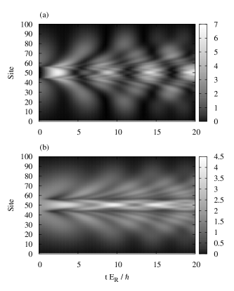
Figure 1: Average number of bosons. In both simulations the hopping among sites decreases inversely with the distance, starting with $R_{i,i\pm 1}=0.3E_{R}$ for first neighbours. $E_{R}$ is an energy reference. We assume that the condensate is trapped in a parabolic potential with $\Omega=0.00046E_{R}$ Rey . (a) the initial state corresponds to two condensates separated by a potential barrier. This state is obtained by calculating the ground state of a chain for the specified parameters plus a potential in the middle given by $R_{i,i}=1000E_{R}$, for $i=45-55$. The dynamics is generated by turning the barrier off. (b) Starting from the ground state of the Hamiltonian, a potential barrier like in (a) is turned on.

In order to illustrate the method, simulations in chains of 100 sites and 100 bosons are shown in Fig. 1. Condensate dynamics is induced by tuning a potential barrier in the middle, as experimentally proposed in Chang . As a consequence, different evolution patterns emerge depending on how and when the potential barrier is switched on and off. From Fig. 1 we observe that wave trains travelling outwards are formed moments after a boson bulk appears in the centre of the chain. Then, a new bulk reassembles and the process starts again. The wave patterns generated in this way are consistent with the observations reported in Chang , where boson trains emerge as a result of the rich dynamics generated in the experiment. Moreover, the computational cost involved in the simulations presented above is minimal compared to TEBD computations, where the chain must be swept many times until ground state convergence is achieved.

When several summations of creation operators acting on the vacuum are involved, as for instance in systems originally arranged with bosons on different positions, state folding can also be implemented. For the shake of simplicity, let us focus on just two summations so that the state can be written as,

$$\left(\overbrace{\sum_{k=1}^{N}c_{k}\hat{a}_{k}^{\dagger}}^{S_{2}}\right)^{M_{2}}\left(\overbrace{\sum_{l=1}^{N}z_{l}\hat{a}_{l}^{\dagger}}^{S_{1}}\right)^{M_{1}}|0\rangle,$$ (4)

where $M_{1,2}$ account for the corresponding number of bosons. $S_{1}$ can be folded using the standard technique, taking into account that the coefficients in $S_{2}$ are also affected in the process. After this, we can fold $S_{2}$, but this time folding $\hat{a}_{2}^{\dagger}$ in $S_{2}$ would inevitably unfold $S_{1}$. Therefore, the folded state acquires the following form,

$$|g\rangle=\left(\hat{a}_{1}^{\dagger}\right)^{M_{2}}e^{-i\phi_{1}\hat{Q}_{1}}\left(\hat{a}_{1}^{\dagger}\right)^{M_{1}}|0\rangle.$$ (5)

In order to write $|g\rangle$ in block decimation notation, we first write $|M_{1},0,...,0\rangle$ and apply $e^{-i\phi_{1}\hat{Q}_{1}}$. When the state obtained in this way is written with explicit reference to the local coordinates of the first position, we can apply $\left(\hat{a}_{1}^{\dagger}\right)^{M_{2}}$ , giving the following result comment1 ; comment2 ,

$$|g\rangle=\sum_{\gamma=1}^{N_{\gamma}}\Gamma_{1\gamma}^{[1]j}\lambda_{\gamma}^{[1]}\sqrt{(j+M_{2})!}|j+M_{2}\rangle|\gamma\rangle^{[2-N]}.$$ (6)

From which the canonical coefficients of state $|g\rangle$ can be directly obtained, namely, ${\Gamma^{\prime}}_{1\gamma}^{[1]j+M_{2}}=\Gamma_{1\gamma}^{[1]j}$ and ${\lambda^{\prime}}_{\gamma}^{[1]}=\sqrt{(j+M_{2})!}\lambda_{\gamma}^{[1]}$ $+$ normalization. It is important to note that this operation, while not unitary, does not modify the original configuration of Schmidt vectors across the chain. To see this, consider first the Schmidt vectors corresponding to the first site, $\{|\gamma_{i}\rangle^{[1]}\}$. Because Hamiltonian (1) preserves the total amount of particles, these vectors each have a definite number of bosons associated with them. Consequently, applying $\hat{a}_{1}^{\dagger}$ lifts the state occupation by one. These lifted kets are orthogonal and therefore valid Schmidt vectors of the whole updated state. On the other hand, any other Schmidt decomposition of the system is made of only one vector to the left and one vector to the right, since there is no boson at all between sites $3$ and $N$. As a result, lifting the local basis in the first site cannot alter the topology of the original decomposition.

In order to illustrate how these ideas can be applied to solve challenging problems, we first introduce our dynamical model analytically so as to synthesize some useful results. Consider the case where $M$ bosons are sent from one end of the chain to the other Plenio ; Franco under the presence of a potential barrier in the central part. Evolution is therefore given by $\hat{\alpha}_{1}^{M}|0\rangle$. We assume that the dynamics is described by a matrix $\hat{R}=\hat{J}_{x}+\epsilon e^{-\beta\hat{J}_{z}^{2}}$, where $\hat{J}_{x,y,z}$ are the standard angular momentum operators. In this way, $\hat{J}_{x}$ induces transmission of bosons from one end of the chain to the other while the term proportional to $\epsilon$ represents a perturbation symmetrically localized over the central part of the chain. $\hat{R}$ acts on the set of eigenvectors of $\hat{J}_{z}$, which are associated to the original operators according to $|j,m\rangle\rightarrow\hat{a}_{j-m+1}^{\dagger}$, where $j=\frac{N-1}{2}$. Similarly, the evolution of operator $\hat{\alpha}_{1}$ can be studied by following the time evolution of ket $|j,j\rangle$:

$$|\psi(t=\pi)\rangle=e^{-i\pi(\hat{J}_{x}+\epsilon e^{-\beta\hat{J}_{z}^{2}})}|j,j\rangle$$ (7)

$$\approx|j,-j\rangle-i\epsilon\int_{0}^{\pi}dte^{-i(\pi-t)\hat{J}_{x}}e^{-\beta\hat{J}_{z}^{2}}e^{-it\hat{J}_{x}}|j,j\rangle,$$

In latter equation we have expanded the time evolution operator to first order in $\epsilon$. The integral can also be written as

$$\int_{0}^{\pi}dte^{-i(\pi-t)\hat{J}_{x}}e^{-\beta\hat{J}_{z}^{2}}e^{i(\pi-t)\hat{J}_{x}}e^{-i\pi\hat{J}_{x}}|j,j\rangle$$

$$=\int_{0}^{\pi}dte^{-\beta(\cos(t)\hat{J}_{z}-\sin(t)\hat{J}_{y})^{2}}|j,-j\rangle$$ (8)

$$=\frac{1}{\sqrt{4\pi\beta}}\int_{-\infty}^{\infty}dxe^{-\frac{x^{2}}{4\beta}}\int_{0}^{\pi}dte^{ix(cos(t)\hat{J}_{z}-sin(t)\hat{J}_{y})}|j,-j\rangle.$$

In the last line we have used the well known identity $\int_{-\infty}^{\infty}dxe^{-(ax^{2}+bx)}=\sqrt{\frac{\pi}{a}}e^{\frac{b^{2}}{4a}}$. We can calculate the action of angular momentum operators in the integral above using Schwinger’s model of angular momentum. To this end, we define two sets of creation and annihilation operators $\hat{a}_{+},\hat{a}^{\dagger}_{+}$ and $\hat{a}_{-},\hat{a}^{\dagger}_{-}$, in terms of which $\hat{J}_{z}=\frac{1}{2}(\hat{a}_{+}^{\dagger}\hat{a}_{+}-\hat{a}_{-}^{\dagger}\hat{a}_{-})$, $\hat{J}_{+}=\hat{a}_{+}^{\dagger}\hat{a}_{-}$, $\hat{J}_{-}=\hat{a}_{-}^{\dagger}\hat{a}_{+}$ and $|j,m\rangle=\frac{(\hat{a}_{+}^{\dagger})^{j+m}(\hat{a}_{-}^{\dagger})^{j-m}}{\sqrt{(j+m)!(j-m)!}}|0\rangle$. In this way integral (8) becomes,

$$\frac{j}{\sqrt{(2j)!4\pi\beta}}\int_{-\infty}^{\infty}dye^{-\frac{j^{2}y^{2}}{4\beta}}\int_{0}^{\pi}dte^{ij^{2}x\cos(t)}\times$$ (9)

$$\left(\hat{a}_{+}^{\dagger}\sin\left(\frac{jy\sin(t)}{2}\right)+\hat{a}_{-}^{\dagger}\cos\left(\frac{jy\sin(t)}{2}\right)\right)^{2j}|0\rangle,$$

where we have performed the variable change $x=jy$. We then use the binomial expansion and obtain a sum of integrals. We can expand the trigonometric functions in power series with little loss in accuracy when the negative exponential in the first integral suppresses the contribution of the second integral for relatively high values of $y$. This can be guaranteed as long as $\beta\ll\frac{j}{2}$, which accounts for a perturbation operating on a section of the chain much smaller than the system size. With this approximation equation (9) gives,

$$\frac{j}{\sqrt{4\pi\beta}}\int_{-\infty}^{\infty}dye^{-\frac{j^{2}y^{2}}{4\beta}}\sum_{k=0}^{2j}\sqrt{\binom{2j}{k}}\left(\frac{y}{2}\right)^{\frac{2j-k}{2}}\times$$

$$\Gamma\left(\frac{2j-k}{2}+\frac{1}{2}\right)J_{\frac{2j-k}{2}}(j^{2}y)|j,j-k\rangle,$$ (10)

which can be integrated using the asymptotic properties of the Bessel functions. So, replacing state vectors by operators we obtain,

$$\hat{\alpha}_{1}(t=\pi)=\hat{a}_{N}^{\dagger}-i\epsilon\sum_{k=0}^{2j}\sqrt{\binom{2j}{k}}\frac{\Gamma\left(\frac{2j-k}{2}+\frac{1}{2}\right)^{2}}{\Gamma\left(\frac{2j-k}{2}+1\right)}\times\beta^{\frac{2j-k}{2}}\hat{a}_{k+1}^{\dagger}.$$

Figure 2: Entanglement between the ends vs. $\frac{\mu}{N}$, the normalized intensity of the potential barrier, $\mu=\epsilon e^{-\frac{\beta}{4}}$ (arbitrary energy units), in a chain of 100 sites. The right axis coordinates correspond to the solid line, the amount of bosons on the ends divided by $M$. In this case curves corresponding to different number of bosons are very similar and therefore they all collapse in one single line. Inset. Intensity of entanglement maxima in the main figure as a function of the number of bosons.

Consequently, for small $\beta$, operator $\hat{\alpha}_{1}$ will generate a particle configuration exponentially localized around the end opposite to the position where particles were initially localized, that is, particles are efficiently transferred from one end to the other. On the other hand, for larger $\beta$ the main contribution will come from $\hat{a}_{1}^{\dagger}$ as well as from $\hat{a}_{N}^{\dagger}$. Hence particles will occupy both ends with little spreading over intermediate sites. Physically, large $\beta$ means the perturbation remains tightly localized in the centre of the chain. In this case one can think that when the particles get across the centre they have a well defined momentum and the perturbation simply acts as a thin wall that causes reflection without altering the wave packet shape. As a result, particles reflected preserve the coherence necessary to be drifted back into their original chain terminal. This phenomenon can be used to efficiently generate entanglement among colliding particles. Ideally, boson packets initially prepared far away from each other in a separable state interact in the middle of the chain via a local potential proportional to the number of boson on the central positions. Some time after the interaction, the majority of bosons turn up on the original positions, but this time these bosons display long range entanglement. This process has been simulated using the two-sum-folding technique previously introduced. So, we solve equation (2) and insert this solution in the expression that determine the initial state as previously specified. Then, for a time equal to half a period we set the quantum state in MPS representation and find the entanglement between the ends of the chain as measured by log-negativity LogN ; ResBos . Here we study chains with $N$ even and therefore a potential barrier is considered in two central sites, but in chains with $N$ odd a highly localized perturbation can be modelled taking one single central site. From Fig. 2 it can be seen that particle collection is highly efficient, with more than $99\%$ of particles collected on the terminals after the interaction. Similarly, entanglement generation is maximally efficient in the range $0.5<\mu/N<1.5$ (see Fig.2 caption for the definition of $\mu$) while the maximum amount of entanglement grows logarithmically as a function of the total number of bosons. This logarithmic behaviour can be studied applying folding techniques. To this end, consider the dynamics generated by $\hat{\alpha}_{1}^{\frac{M}{2}}\hat{\alpha}_{N}^{\frac{M}{2}}|0\rangle$. Because bosons get entangled mainly on the central part of the chain where the particle packets interact, we focus on the form of $\alpha$-operators for a time equal to a quarter period, when the boson packets become symmetrically spread along the chain and therefore $\hat{\alpha}_{1}(\frac{T}{4})=\hat{\alpha}_{N}(\frac{T}{4})$ for a chain without wall. Consequently, the particle distribution adopts the form of Eq. (3), but this time the the $c_{k}$’s are determined by the coupling constants and the strength of the barrier, both considered general up to symmetry. As entanglement between both halves of the chain is independent of unitary transformations on either half-chain block, we can operate on the state using the same transformations employed previously to fold the quantum state as long as we do not operate on pairs of creation operators belonging to different half-chain blocks. In this case, the result of the reduction is trivial and can be written as $(\hat{a}_{1}^{\dagger}+\hat{a}_{2}^{\dagger})^{M}|0\rangle$. Entanglement can be calculated expanding this expression and noticing that as a result we obtain a genuine Schmidt decomposition with coefficients $c_{k}=\sqrt{\frac{1}{2^{M}}\frac{M!}{(M-k)!k!}}$. Hence, log-negativity can be worked out by replacing the binomial distribution by a normal Gaussian. This gives $E_{N}\sim\frac{1}{2}log_{2}(2\pi)+\frac{1}{2}log_{2}(M)$. Moreover, assuming that the interaction among bosons takes place in a time scale much smaller than the transfer time, we can take this result as an estimation of entanglement when the particles reach the chain ends. The discrepancy with the fitting constants in Fig. 2 is due to to the approximations involved in getting $E_{N}$. However, logarithmic growing as well as highly efficient particle collection are positively verified by the numerical analysis. Finally, we would like to point out that the methodology presented in this work can be applied to analogous situations in spin chains or fermion arrangements. Non linear effects, while less amenable to exact analytical solution, could be considered by solving the Gross-Pitaevskii equation and then treating the coefficients describing the wave function as the $c_{k}$’s of Eq. (3). Additionally, the method can be used in combination with TEBD, for example in quench-like problems where repulsion is suddenly turned on. JR acknowledges an EPSRC-DHPA scholarship.

References

- (1) G. Vidal, Phys. Rev. Lett. 91, 147902 (2003); G. Vidal, Phys. Rev. Lett. 93, 040502 (2004); A. Daley et al, J. Stat. Mech. P04005, (2004).
- (2) M.B. Plenio et al, New J. Phys. 6, 36 (2004); Lian-Ao Wu et al, arXiv:0902.3564
- (3) J.J. Chang et al, Phys. Rev. Lett. 101, 170404 (2008).
- (4) A.M. Rey et al, Phys. Rev. A 72, 033616 (2005); S. Montangero et al, Phys. Rev. A 79, 041602 (2009).
- (5) G. Vidal and R. Werner, Phys. Rev. A 65, 032314 (2002).
- (6) J. Reslen et al, Europhys. Lett. 69, 8 (2005)
- (7) J. Reslen and S. Bose, arXiv:0812.0303, to appear in PRA.
- (8) C.K. Law, Phys. Rev. A 70, 062311 (2004); F. Schmuser and D. Janzing, Phys. Rev. A 73, 052313 (2006); M. Lewenstein et al, arXiv:0901.2836.
- (9) C. Di Franco et al, Phys. Rev. Lett. 101, 230502 (2008); S.R. Clark et al, New Jour. Phys. 7 (2005) 124.
- (10) D. Jaksch et al, Phys. Rev. Lett. 82, 1975 (1999).
- (11) F. Verstraete et al, Adv. in Phys. 57, 143-224 (2008)
- (12) In writting in this way, we have used the properties of the canonical decomposition as described in Ref. vidal1 . Specifically, we exploit the fact that the elements of tensor can be seen as the components of the whole quantum state given in terms of the local basis, i.e., the occupation number, and the Schmidt vectors obtained when partitioning the chain to the sides of the place under study.
- (13) In this expression we have implicitly assumed a functional dependece between and due to conservation properties. See Ref.ResBos for a detailed discussion on this matter.