Control of unstable macroscopic oscillations in the dynamics of three coupled Bose condensates

Abstract

We study the dynamical stability of the macroscopic quantum oscillations characterizing a system of three coupled Bose-Einstein condensates arranged into an open-chain geometry. The boson interaction, the hopping amplitude and the central-well relative depth are regarded as adjustable parameters. After deriving the stability diagrams of the system, we identify three mechanisms to realize the transition from an unstable to stable behavior and analyze specific configurations that, by suitably tuning the model parameters, give rise to macroscopic effects which are expected to be accessible to experimental observation. Also, we pinpoint a system regime that realizes a Josephson-junction-like effect. In this regime the system configuration do not depend on the model interaction parameters, and the population oscillation amplitude is related to the condensate-phase difference. This fact makes possible estimating the latter quantity, since the measure of the oscillating amplitudes is experimentally accessible.

1 Introduction

Since the first observation of Bose-Einstein condensates (BECs) in dilute weakly interacting gases of bosons in 1995, great efforts both experimental and theoretical have been addressed on this subject. Thus nowadays, thanks to the impressive progress of experimental techniques, BECs represent a source of inspiration for new challenging problems in quantum physics. A notable aspect inherent in the dynamics of coupled BECs is that the nonlinear character of their equations of motion entails a particularly rich phenomenology where nonlinear effects including chaos can be studied in a quantum environment. Among the latter, in recent experiments have been observed phenomena such as super-fluidity [1], Josephson tunneling [2] and atom optics [3].

If the recent past has been prolific of experiments on BECs arranged into arrays with huge number (of the order of several hundreds) of condensates, at the present, the experiments on chains with a few interacting BECs (of the order of several unities) has received a limited attention [4]-[8] despite the increasing amount of theoretical work devoted to such systems. Over the last few years, work on small-chain models has been focused in particular on the two-well system (dimer) [9]-[13] and the three-well system (trimer) [14], [15] while their many-well generalization has been studied in [16]-[21]. The theoretical prediction of macroscopic effects such as coherent atomic tunneling [9], population self-trapping [22], and Josephson junction effect [23], have been confirmed by recent observations in the experimental realization of the dimer [4]-[8].

These results stimulate the theoretic study of the BEC small chains in order to predict new macroscopic effects that, in addition to furnishing a deeper insight of stability properties and an increased control of systems, open the possibility of designing significant experiments. In this respect, the recent experimental technique discussed in [5, 4] and successfully applied to realize a two-well system provides an extremely effective tool for engineering small arrays. The superposition of a parabolic confining potential to a linear optical lattice allows one to select two wells (dimer) with possibly different depths by changing the parabola position and amplitude. Likewise, a simple, suitable change of the latter should enable one to select $M$-well arrays, with $M$ arbitrary, whose (local) potentials feature a parabolic profile. The trimer case is thus very promising in that, in addition to represent a practicable experimental objective, it exhibits behaviors typical of more complex arrays. In fact, while the simplest BEC array (the dimer) features an integrable dynamics [24], in the trimer case the apparently harmless addition of a further coupled condensate is sufficient to make the system nonintegrable. As a consequence, the trimer displays strong dynamical instabilities in extended regions of the phase space [25] and a whole new class of behaviors including chaos. In general, unstable behaviors have been found in condensates subject to kicked pulses [36] or to an anisotropic trapping potential [37] and within soliton dynamics [38].

Concerning the trimer, a conspicuous number of recent papers has addressed various aspects of its dynamics. These include, within a mean-field approach, the occurrence of a transistor-like behavior [26], and the self-trapping [27] in a triple-well asymmetric trap of repulsive bosons, the ring-trimer dynamics with attractive interaction in the presence of a single on-site defect [28], and the chaos control through an external laser pulse [29]. Recently, the dynamical instability has been studied in terms of quasimomentum modes for a $5$-well semiclassical Bose-Hubbard model including a linear potential [30]. Also, more related to purely quantum properties, second-quantized models of the trimer have been considered to study the properties of quantum states relevant to interwell particle exchange [31] and entanglement [32], the semiclassical quantization of the Bogoliubov spectrum [33], the structural changes of trimer eigenstates in terms of the tunneling parameter [34], and the occurrence of vortex-like states [35].

In the present paper we study the classical dynamics of an asymmetric open trimer (AOT) made of three coupled BECs arranged into an open chain geometry, where both the interwell tunneling amplitude $T$ and the relative depth $w$ of the central well, are regarded as adjustable parameters. Our objective is to evidence several macroscopic effects that can take place in the AOT dynamics to provide a useful guide for future experiments. In section 2 we introduce the semiclassical equations of the trimer mean-field dynamics. In section 2.1, after determining the solutions relevant to the fixed points of motion equations, i. e. the proper modes of trimer dynamics, we focus mostly on establishing, via standard procedures, their stability character for experimentally significant values of effective parameters $\tau:=T/UN$ and $\nu:=w/UN$, where $U$ and $N$ are the effective interatomic scattering and the total boson number, respectively. In section 3 we review the (three) stability diagrams (one for each class of fixed points) that summarize characters and properties of fixed points. These supply an exhaustive, operationally valuable, account of the system stability properties and allow to determine the stable/unstable charater of the system evolution for initial conditions situated, in the phase space, close to a given fixed point. Both the derivation and the use of such diagrams, rapidly sketched in [39], are discussed here (and in the relevant appendices) with some detail together with various new applications.

By using the stability diagrams as a map for detecting the critical behaviors of trimer, in section 4 we find parameter-tuned macroscopic effects (both in the dimeric and nondimeric regime) and evidence some features that may prove experimentally relevant. Such effects are shown to arise when crossing either the boundaries of regions with different stability characters or the boundaries of forbidden regions or, finally, by exploiting the coalescence/bifurcation mechanism characterizing certain fixed points. In section 5 we consider the special case of $\pi$-like states relevant to the fixed points of the regime charaterized by a central depleted well. We investigate the unexpected relation between the average population oscillations and the initial phase difference of the lateral condensates, suggesting a possible experiment. Finally, section 6 is devoted to make some concluding remarks.

2 Dynamical equations of the AOT and fixed points

The quantum Hamiltonian of the AOT on a linear chain reads [16]

$$H_{3}=\sum^{3}_{i=1}(Un_{i}^{2}-vn_{i})-wn_{2}\!-\!\frac{{}_{T}}{{}^{2}}\left[a^{\dagger}_{2}(a_{1}+a_{3})\!+\!\rm{H.C.}\right]$$ (1)

where site boson operators $a_{i}^{\dagger},a_{i}$ satisfy standard commutators $[a_{i},a^{\dagger}_{k}]=\delta_{ik}$, $n_{i}=a_{i}^{+}a_{i}$, $v$ is the energy offset of the wells, $w$ is the central-well relative depth, $T$ is the hopping amplitude and $U\simeq 2\pi a\hbar^{2}/m$ ($a$ the scattering length, $m$ the boson mass) is the on-site boson interaction. The total boson number $N=\sum_{i}n_{i}$, commutes with Hamiltonian (1). The exact form of parameters $U$ and $T$ is calculated in [40] showing how such quantities depend on $m$, on the laser wavelength $\lambda$, and on the potential depth $V_{0}$ of potential $V_{op}(x)=V_{0}\sin^{2}(2\pi x/\lambda)$ determining the optical lattice. The 3-well linear system, obtained by superposing the optical potential to parabolic potential $V_{p}(x)=m\omega^{2}x^{2}/2$ confining bosons [4], [5], is expected to have lateral wells with depth $v$ smaller then the central-well depth $v+w$ due to the presence of the parabolic potential. The dynamics of the AOT with strong tunnelling amplitudes ($T/U>>1$) and large average numbers of atoms per well can be described by the mean-field form of (1). The method developed in [41] combines the coherent-state picture of quantum systems with the time-dependent variational approach [42] providing the semiclassical version of quantum model (1) in which the dynamical canonical variables are the expectation values $z_{i}:=\langle Z|a_{i}|Z\rangle$, $z^{*}_{i}:=\langle Z|a^{+}_{i}|Z\rangle$. The so-called trial macroscopic wave function $|Z\rangle$ is standardly assumed to be $|Z\rangle=\prod_{i}|z_{i}\rangle$, where $1\leq i\leq 3$ and $|z_{j}\rangle$ are the Glauber coherent states such that $a_{i}|z_{i}\rangle=z_{i}\,|z_{i}\rangle$ for each $i$. Then, the resulting mean-field Hamiltonian reads

$${\cal H}_{3}=\sum_{j=1}^{3}\left[U|z_{j}|^{4}-v|z_{j}|^{2}\right]-w|z_{2}|^{2}-\frac{{}_{T}}{{}^{2}}[\,z_{2}^{*}(z_{1}+z_{3})+{\rm C.C.}]\,,$$ (2)

which, through the Poisson brackets $\{z_{j}^{*},z_{k}\}=\frac{i}{\hbar}\delta_{jk}$, yields the dynamical equations

$$\left\{\begin{array}[]{ll}i\hbar\dot{z}_{j}\!=\!\left(2U|z_{j}|^{2}-v\right)z_{j}-\frac{T}{2}z_{2}&j=1,3\\ i\hbar\dot{z}_{2}\!=\!\left(2U|z_{2}|^{2}-v\!-\!w\right)z_{2}\!-\!\frac{T}{2}\left(z_{1}\!+\!z_{3}\right)&\end{array}\right.$$ (3)

The validity of such a semiclassical picture is confirmed experimentally [4], [5] for the time scale (hundreds of milliseconds) of the macroscopic oscillations in a two-well system. The effect of approximating the system state $|Z\rangle$ through a product of localized (coherent) states $\prod_{i}|z_{i}\rangle$ appears on a much longer time scale [43] when $|Z\rangle$ must be expressed as a superposition of Fock states $|{\vec{n}}\rangle=|n_{1},n_{2},n_{3}\rangle$ ($a^{+}_{i}a_{i}|{\vec{n}}\rangle=n_{i}|{\vec{n}}\rangle$) to include (quantum) delocalization effects. An early analysis of equations (3) for $w=0$ is reported in [44], [45]. It is easy matter to check that system (3) embodies the conservation of boson total number $N=\Sigma_{j}|z_{j}|^{2}$, namely $\{N,H\}=0$. Constant $N$ can be exploited to introduce new rescaled variables $Z_{j}\equiv z_{j}e^{-ivt/\hbar}/{\sqrt{N}}$ whose evolution is governed by

$$\left\{\begin{array}[]{ll}iZ^{\prime}_{j}\!=\!2|Z_{j}|^{2}\,Z_{j}-\frac{\tau}{2}Z_{2}&j=1,3\\ iZ^{\prime}_{2}\!=\!\left(2|Z_{2}|^{2}-\nu\right)Z_{2}-\frac{\tau}{2}\left(Z_{1}\!+\!Z_{3}\right)&\end{array}\right.$$ (4)

where

$$\quad\nu={w}/{(UN)},\quad\tau={T}/{(UN)},\quad{\tilde{t}}={UNt}/{\hbar}\,,$$ (5)

and the prime denotes derivation with respect to the rescaled time variable $\tilde{t}$. This shows that the two significant parameters of the trimer dynamics are $\nu$ and $\tau$ (namely, at fixed $N$, $w/U$ and $T/U$), parameter $v$ being incorporated in the time dependent factor $e^{-ivt/\hbar}$ of new variables $Z_{j}$. Furthermore, it is easy to verify that the condition $z_{1}(t)=z_{3}(t)$ is valid for $t>0$ (or, equivalently, that $Z_{1}(\tilde{t})=Z_{3}(\tilde{t})$ holds for every $\tilde{t}>0$) if, initially, $z_{1}(0)=z_{3}(0)$. Such a condition identifies an integrable subregime where the lateral condensates have the same population and phase (see, e. g., [44], [46] and [47]) which in the following we shall refer to as dimeric regime.

2.1 Fixed points

We can get insight about the behaviour of the system in different dynamical regimes through the study of special exact solutions along with their stability character. With the latter we mean the simplest (single mode) periodic orbits in the phase space of the form $Z_{j}(t^{\prime})=x_{j}e^{imt^{\prime}}$. Substituting the latter in equations (4) provides the equations for variables $x_{j}$. Such equations can be equivalently obtained from $i{Z^{\prime}}_{j}=0=\{Z_{j},{\tilde{H}}-m{\tilde{N}}\}$ with ${\tilde{H}}={\cal H}_{3}(Z_{i},Z^{*}_{i})$, where the chemical potential $m$, a Lagrange multiplier, allows one to include the conserved quantity ${\tilde{N}}=\sum_{i}|Z_{i}|^{2}=1$ derived from the total boson number $N=\sum_{i}|z_{i}|^{2}$. Owing to the condition ${Z^{\prime}}_{i}=0$ we name fixed-point equations the equations determining $x_{i}$, $i=1,2,3$. These have the form

$$0=\left(2\,x_{j}^{2}-m\right)\,x_{j}-\frac{\tau}{2}\,x_{2}\,,\,\,\,0=\left(2\,x_{2}^{2}-m-\nu\right)\,x_{2}-\frac{\tau}{2}\,\left(x_{1}+x_{3}\right)$$ (6)

where $j=1,3$ and the fixed-point coordinates ${x_{j}}$ are normalized to unity: $\sum_{j}x_{j}^{2}=1$. In equation 6 we have exploited the system symmetry, inherited from equations 4, under a global phase shift $x_{j}\mapsto x_{j}\exp(i\Phi)$ to restrict coordinates ${x_{j}}$ (which are in principle complex numbers) to the real axis. Let us summarize the solutions of system (6).

Central depleted well. This parameter-independent solution is obtained when the central well is strictly depleted, that is $x_{2}=0$, whereas the lateral ones have the same population and opposite phases. Due to the constraint on the number it must necessarily be $x_{1}=-x_{3}=\pm\sqrt{m/2}=\pm 1/\sqrt{2}$, $m=1$. In summary

$$x_{1}=-x_{3}=\pm 1/\sqrt{2}\,,\quad x_{2}=0\,.$$ (7)

We shall refer to this solution as central depleted well (CDW). Since configurations where either one or both of the lateral condensates have zero population are forbidden by equations (6), we are left with the following two possibilities.

Dimeric solutions. Similar to (3) and (4), equations (6) possess dimeric solutions characterized by $x_{2}\neq 0$ and $x_{1}=x_{3}\neq 0$. These solutions can be expressed via the polar representation

$$x_{1}=x_{3}={\cos\theta}/{\sqrt{2}}\,,\qquad x_{2}=\sin\theta\,.$$ (8)

Introducing this parametrization in (6) one finds that the tangent $\tan\theta=:{\alpha}$ of the angular coordinate $\theta$ identifying each fixed point is given by the real roots of

$${\cal P}({\alpha};\tau,\nu)\equiv{\alpha}^{4}+\frac{A_{\nu}}{\tau}{\alpha}^{3}-\frac{B_{\nu}}{\tau}{\alpha}-1=0\,,$$ (9)

with $A_{\nu}=\sqrt{2}(2-\nu)$, $B_{\nu}=\sqrt{2}(1+\nu)$. In the following we shall refer to this class of solutions as dimeric fixed points (DFP) whose derivation is discussed in A.1.

Non-dimeric solutions. The remaining single-mode solutions of system (6), characterized by $x_{1}\neq x_{3}$, $x_{j}\neq 0$, will be referred to as non-dimeric fixed points (NFP). In this case it is appropriate to switch to the alternative set of coordinates $X_{1}=(x_{1}+x_{3})/{\sqrt{2}}$, $X_{2}=x_{2}$, and $X_{3}=(x_{1}-x_{3})/{\sqrt{2}}$ before setting

$$X_{1}=R\cos\theta,\quad X_{2}=R\sin\theta\,.$$ (10)

In this case the radial coordinate $R$ reads

$$R({\alpha};\,\tau)=\sqrt{\frac{(1+\alpha^{2})(2\sqrt{2}-\alpha\,\tau)}{2\sqrt{2}(2+\alpha^{2})}}\,,\quad{\alpha}=\tan\theta:=\frac{X_{2}}{X_{1}}$$ (11)

and depends on the Hamiltonian parameter $\tau$ and on parameter $\alpha$. By introducing this parametrization in system (6) one finds that $\alpha$ is given by the real roots of

$${\cal P}({\alpha};\tau,\nu)\equiv{\alpha}^{4}+\frac{A_{\nu}}{\tau}{\alpha}^{3}-\frac{B_{\nu}}{\tau}{\alpha}-\frac{4}{3}=0\,,$$ (12)

where $A_{\nu}={2\sqrt{2}(2-\nu)}/{3}$, $B_{\nu}={4\sqrt{2}(1+\nu)}/{3}$. Since the physical solutions of system (6) have to be real it is clear that the roots which make $R({\alpha})$ or

$$X_{3}(\alpha)\!=\!\pm\sqrt{1-X_{1}^{2}-x_{2}^{2}}\!=\!\pm\sqrt{\frac{4\!+\!\sqrt{2}\alpha(1+\tau\alpha^{2})}{4(2+{\alpha}^{2})}}$$ (13)

imaginary, must be discarded. The next section contains a qualitative discussion of the three stability diagrams describing the entire set of solutions of system (6) for any choice of $\tau$ and $\nu$. A detailed derivation of such fixed points is given in A.2.

3 Stability diagrams

The stability diagrams introduced in [39] allow one to know both number and stability character of the fixed points of trimer dynamics for any choice of significant parameters $\tau$ and $\nu$. In the previous section we have shown that vector ${\bf x}=(x_{1},x_{2},x_{3})$ describing a fixed point can be parametrized by the angular coordinate $\theta$ of the two-dimensional polar representations (8), and (10) and (11) for the DFP and the NFP, respectively. To determine parameter $\theta$ (and thus the vector ${\bf x}$ relevant to a given fixed point) we must find the roots of the fourth-degree polynomial

$${\cal P}(\alpha;\tau,\nu)={\alpha}^{4}+\frac{A_{\nu}}{\tau}{\alpha}^{3}+\frac{B_{\nu}}{\tau}{\alpha}+C=0$$ (14)

in the unknown quantity $\alpha=\tan\theta$. This allows one to determine $\alpha=x_{2}/\sqrt{2}x_{1}$ in the dimeric case with $C=-1$ (see (9)), and $\alpha=x_{2}/\sqrt{2}(x_{1}+x_{3})$ in the non-dimeric case with $C=-4/3$ (see (12)). In the latter case vector $\bf x$ is obtained by using the constraint $x_{1}^{2}+x_{2}^{2}+x_{3}^{2}=1$. Therefore, for a given value of parameters $\tau$ and $\nu$, the number of roots of (14) establishes how many DFP and NFP there exist. This information is summarized in figures 1 and 3.

The stability character of the fixed points solving equations (6) is depicted in the stability diagrams of figures 2 and 4 for the DFP and the NFP case, respectively. In such figures any point in the plane $\theta-\tau$ is implicitly associated to a definite value of parameter $\nu$, owing to equation (14). This can be seen by rewriting (14) as

$$\tau[\tan(\theta);\nu]=-\frac{\left[A_{\nu}\tan^{2}(\theta)+B_{\nu}\right]\tan(\theta)}{\tan^{4}(\theta)+C}\,,$$ (15)

which, for a given value $\nu=\tilde{\nu}$, defines a curve $\tau[\tan(\theta);\tilde{\nu}]$ in the plane $\theta$-$\tau$ consisting of two or more non-connected branches, both in the dimeric ($C=-1$) and the non-dimeric case ($C=-4/3$). At the operational level, in both figures, for a given choice $\tau\equiv\tilde{\tau}$ and $\nu\equiv\tilde{\nu}$, configuration parameter $\theta$ can be obtained by intersecting the curves $\tau[\tan(\theta);\tilde{\nu}]$, for the dimeric and non-dimeric case, and the straight line $\tau=\tilde{\tau}$. Once (triplet $\tau$, $\nu$, $\theta$ of) a fixed point has been identified, its stable/unstable character can be evinced from figures 2 or 4 thanks to the colour corresponding to a given value of $\theta$ and $\tau$ (see the relevant figure captions). The linear stability analysis determining the character of fixed points (and, in practice, the whole structure of such phase diagrams) is discussed in A.

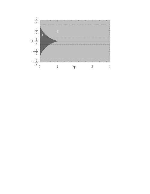
Figure 1: Number of dimeric fixed points on varying parameters $\tau$ and $\nu$. The border of the lobe where four solutions are found is described by (21).

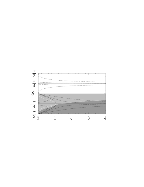
Figure 2: Stability diagram for the dimeric fixed points (DFP). The fixed points belonging to the white, medium grey and dark grey regions are always minima, unstable saddles and maxima, respectively. The latter two regions are divided by the curve $\tau=d(\tan\theta)$ defined in A.1. The tip of the “parabolic” branch moves along the white dashed curve. The white dotted and dashed curves are $d_{1}(\tan\theta)$ and $d_{2}(\tan\theta)$, respectively (see A.1 for details). Note that the curves drawn with diffrent dashing styles, correspond to the five values of $\nu$ selecting the straight horizontal lines reported with the same dashing styles in figure 1.

As an example, in figures 1 and 3 are reported with different dashing styles, five straight horizontal lines corresponding to several values of the $\nu$. The five curves drawn in figures 2 and 4, refer to the straight lines drawn with the same dashing styles in figures 1 and 3, for the dimeric and non-dimeric case, respectively.

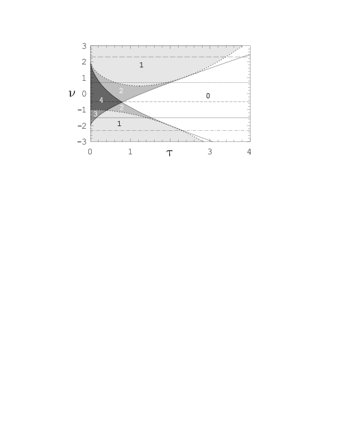
Figure 3: Number of non-dimeric fixed points on varying parameters $\tau$ and $\nu$. The same shade of grey fills regions characterized by the same number of fixed points (shown).

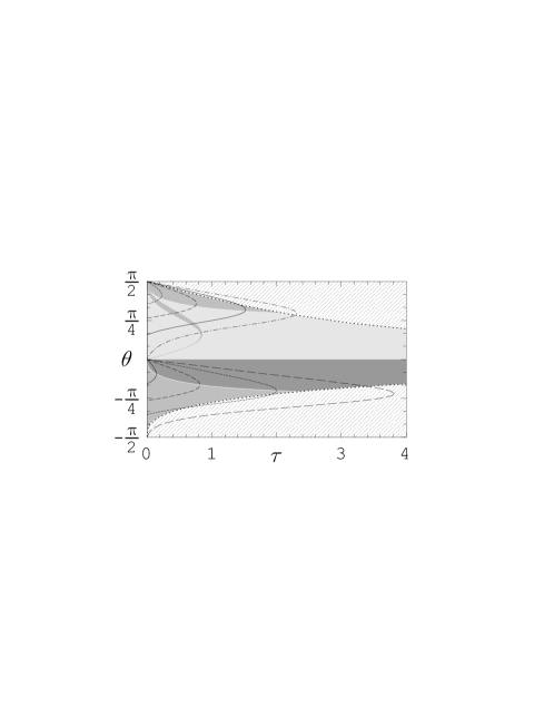
Figure 4: Stability diagram for the non-dimeric fixed points (NFP). The fixed points belonging to the light, medium and dark grey regions are always stable saddles, unstable saddles and maxima, respectively. Note that the white solid curves are the loci of the tips of the two parabolic branches. The patterned regions must be ignored, since the solutions found there yield complex $x_{j}$’s (see A.2 for details). The curves drawn with diffrent dashing styles, correspond to the five values of $\nu$ selecting the straight horizontal lines reported with the same dashing styles in figure 3.

Notice that in general these curves consist of two or more non-connected branches. In the dimeric case there are always two unbounded branches featuring an asymptote at $\theta=+\pi/4$ or at $\theta=-\pm\pi/4$. For $\nu\in[-1,2]$ a further, roughly parabolic, bounded branch appears. This means that for any choice of the parameters $\tau$ and $\nu$ there are always at least two DFPs, and that, for suitable choices of these parameters, two more fixed points appear.

In the non-dimeric case, figure 4, the curves $\tau[\tan(\theta);\nu]$ consist of either one or two bounded parabola-like branches, hence featuring zero, two or four intersection with a constant-$\tau$ straight line. However, for certain values of the parameters, not all of these intersections represent fixed points, i.e. real solutions of system (6). Indeed, as it is discussed in A.2, some of the real roots of polynomial ${\cal P}(\alpha;\tau,\nu)$ –more precisely the ones lying in the patterned regions of figure 4– result in complex-valued solutions of system (6) and therefore must be discarded. In particular, the patterned (forbidden) regions of figure 4 can be shown to correspond to the white region in the $\tau$-$\nu$ plane of figure 3 where no solution is permitted. Figures 2 and 4 also supply important information concerning fixed points and their characteristic energies. Referring to the different colours used in such figures, a fixed point is a (stable) minimum, a stable saddle, an unstable saddle or a (stable) maximum of the energy function depending on whether the region it lies in is white, light grey, medium grey or dark grey.

As we mentioned above, other than the DFPs and the NFPs, a further fixed point, the CDW configuration, is present for any value of $\tau$ and $\nu$. The parameter independence of the relevant configuration ${\bf x}=(1/\sqrt{2},0,-1/\sqrt{2})$, makes the use of a polar representation unnecessary, and allows one to draw its stability diagram in the parameter plane $\tau$-$\nu$ in a direct way. This is illustrated in figure 5.

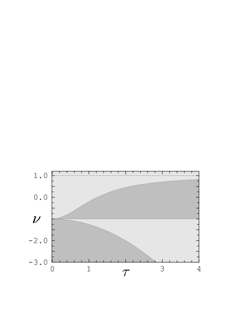
Figure 5: Stability diagram for the CDW saddle point. Note that large stability regions appear (light grey filling). The boundaries are the straight line $\nu=0$ and the curves $\tau=c_{1}(\nu)$ and $\tau=c_{2}(\nu)$, described by (27). The asymptote $\nu=1$ of the latter curve is also displayed (dashed line).

4 Macroscopic effects in the AOT dynamics

A careful look at stability diagrams 2 and 4, in addition to provide, at first glance, number and properties of the fixed points of AOT dynamics for any choice of $\tau$ and $\nu$, allows one to single out at least three ways to produce macroscopic, and hence experimentally observable, effects by means of a simple change of model parameters.

Crossing boundaries of regions with a different character. For suitable choices of $\nu$, curves $\tau[\tan(\theta);\nu]$ may cross the boundary dividing regions with different stability properties. Thus, by slightly and adiabatically changing the Hamiltonian parameters (e.g. the optical potential amplitude) the system can modify significantly its behavior. This is the case of (one of) the asymptotic branches of the dimeric curves, which, for any $\nu>2\sqrt{14}-7\approx 0.48$, crosses the boundary between the maxima and the unstable saddles region (see, e. g., the branch in figure 1 corresponding to $\nu=0.6$ in figure 3). Likewise, in the non-dimeric case, one of the parabola-like branches of curves $\tau[\tan(\theta);\nu]$ always crosses the interesting unstable “isthmus” splitting the large stable (light-grey) region in figure 4, provided that $\nu<2$.

Coalescence/bifurcation of fixed points. At the “tips” of the parabola-like branches of curves $\tau[\tan(\theta);\nu]$, a coalescence/bifurcation effect of pairs of fixed points takes place. Hence, for some values $\tilde{\tau}$ of the hopping parameter it is possible to find a value $\tilde{\nu}$ with two coincident solutions of fixed-point equations located at the parabolic-branch tip. By varying $\nu$, the branch tip moves away from $\tilde{\tau}$, and the coincident solutions either split (i.e. bifurcate) or disappear accordingly. Let us emphasize that in the non-dimeric case (figure 4) the coalescence phenomena always involve fixed points with different stability characters, whereas, in the dimeric case (figure 2) only the coalescence of two fixed points of the same kind may happen, provided that $\nu>2\sqrt{14}-7$ (see next section).

Crossing forbidden-region boundaries. Significant changes in the phase-space structure of the system are expected as well where the non-dimeric curves $\tau[\tan(\theta);\nu]$ cross the boundaries of forbidden zones. Indeed, in this case, a slight change in the parameters may cause the sudden appearance/disappearance of a fixed point. As to the CDW fixed points, which –according to the Hessian signature– is always a saddle, figure 5 clearly shows that it may display an either stable or unstable character, depending on the choice of parameters $\tau$ and $\nu$

Based on these three mechanisms, we discuss the results of several numeric simulations evidencing how macroscopic effects are induced in the AOT dynamics by slight changes in parameters $\tau$ and $\nu$ (similar effects on the stability of the many-well system with $U<0$, of vortexlike modes in a 1D array and of localized modes in a 2D array have been studied in  [48], [20] and [21], respectively). These entail that trajectories based on the same initial configuration may exhibit an either regular or chaotic behavior. The character of the AOT dynamics, can be conveniently investigated by constructing appropriate Poincaré sections within the four-dimensional reduced phase-space spanned by the (reduced) set of canonical variables ${\phi_{1},\xi_{1},\phi_{2},\xi_{2}}$. This reduction is obtained via the canonical transformation $(z_{i},z^{*}_{i})$ $\to(\phi_{1},\phi_{2},\psi,\xi_{1},\xi_{2},N)$, where

$$\begin{array}[]{ll}\phi_{1}=\theta_{2}-\theta_{1},&\xi_{1}=(|z_{2}|^{2}+|z_{3}|^{2}-|z_{1}|^{2})/N,\\ \phi_{2}=\theta_{3}-\theta_{2},&\xi_{2}=(|z_{3}|^{2}-|z_{2}|^{2}-|z_{1}|^{2})/N,\\ \psi=\theta_{3}+\theta_{1},&N=(|z_{1}|^{2}+|z_{2}|^{2}+|z_{3}|^{2}),\\ \end{array}$$ (16)

once the condition $N={\rm const}$ is taken into account and one notices that the $\psi$ evolution is nonautonomous (see [25] for details on the reduced dynamics).

We have numerically integrated the trimer equations of motion in the reduced coordinates, by a first-order bilateral symplectic algorithm. Moreover, we have qualitatively investigated the degree of regularity of the ensuing trajectories by means of Poincaré sections. The latter are obtained by projecting the points belonging to a given submanifold, characterized by a given value of one of the four reduced variables, onto the plane spanned by two of the three remaining variables. All of the Poincaré sections reported in the following refer to a set of trajectories based on an array of starting points surrounding a significant configuration of the system, usually a fixed point, of reduced coordinates $(\tilde{\phi}_{1},\tilde{\xi}_{1},\tilde{\phi}_{2},\tilde{\xi}_{2})$. In every instance the points belonging to the submanifold $\xi_{2}=\tilde{\xi}_{2}$ have been projected onto the $\phi_{1}$-$\xi_{1}$ plane.

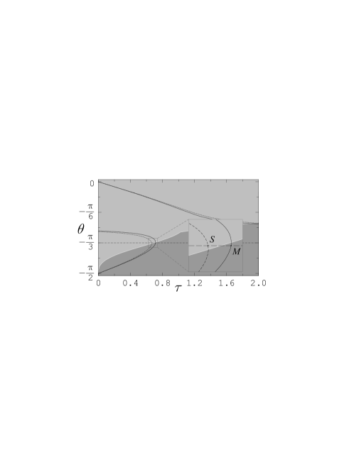
Figure 6: Parameter-induced macroscopic change in the stability of the trimer dynamics. The figure shows a portion of the lower half plane of dimeric stability diagram 2, along with the dimeric $\tau$-curves (see (15), (22)) relevant to $\nu=\nu_{\rm M}=2/3$ (solid) and $\nu=\nu_{\rm S}=17/24$ (dashed). The white dotted and dashed curves appearing in figure 2 have been omitted for clarity. From the figure it is clear that, for both of the considered values of $\nu$, there exists a suitable value of the hopping parameter —$\tau_{\rm M}=7/4\sqrt{6}$ and $\tau_{\rm S}=13/8\sqrt{6}$, respectively — producing a solution at $\theta=-\pi/3$ (horizontal dashed line). Hence slight differences in the parameters may result in different stability characters for the same configuration ($\theta=-\pi/3$). Indeed M is a (stable) maximum, whereas $S$ is an unstable saddle.

4.1 Priming instability in breather-like regular oscillations

The first macroscopic effect we discuss here has been briefly discussed in [39] and concerns the dimeric configuration ${\bf x}=(1/\sqrt{8},-\sqrt{3}/2,1/\sqrt{8})^{\rm t}$, –with $N/8$ bosons in each lateral well and the remaining $3N/4$ in the central one– which is represented by the angular variable, $\theta=-\pi/3$. One can show that the latter is a (dimeric) fixed point provided that $4\sqrt{6}\,\nu+8\,\tau-5\sqrt{6}=0$. Furthermore, such a fixed point is either a maximum or an unstable saddle depending on whether $\nu$ is smaller or larger than the critical value $9\sqrt{6}/32$. This is clearly visible in figure 6, where two different parameter choices $(\tau_{\rm M},\nu_{\rm M})$ and $(\tau_{\rm S},\nu_{\rm S})$, shown with the letters $M$ and $S$, are considered.

The crossing of the boundary separating the stable and unstable regions has evident consequences. The Poincaré sections (reported in [39]) of trajectories, based on a set of points closely surrounding the fixed point under concern $(\phi_{1},\xi_{1},\phi_{2},\xi_{2})=(\pi,3/4,-\pi,-3/4)$, mirror the dramatic change in the dynamical behaviour involved in such a slight parameter change. While choice $(\tau_{\rm M},\nu_{\rm M})$ results in the neat and regular Poincaré sections characterizing a stable fixed point, with choice $(\tau_{\rm S},\nu_{\rm S})$ sections densely fill an area considerably larger than the previous example, despite the relevant trajectories are based on the very same points [39].

4.2 Loss of anti-breather coherence in the isthmus domain

An instability outbreak similar to that discussed above is found in the neighborhood of the “instability isthmus” of the non-dimeric stability diagram 4. Indeed, the possibly present upper branch of the non-dimeric $\tau$ curve always crosses such unstable region. This is the case of four of the five curves plotted in figure 4 and of the curve with $\nu=0$ plotted in figure 7. The inset of figure 7 is a magnification showing fixed points $A$, $B$ and $C$, located in the proximity of the instability “isthmus” for three slightly different values of $\tau$ ($\tau_{\rm A}=0.22$, $\tau_{\rm B}=0.29$ and $\tau_{\rm C}=0.36$). These fixed points correspond to (slightly) different values of coordinate $\theta$, thus the corresponding configurations are quite similar to each other. In these three cases more than $97\%$ of the total population is almost equally shared by the central and one of the lateral condensates. The phases of these condensates are parallel to each other and opposite to that of the remaining, almost empty, condensate. This kind of configuration corresponds to the neighborhood of the reduced-phase-space point with $(\phi_{1},\xi_{1},\phi_{2},\xi_{2})=(0,0.016,\pi,-0.984)$. Figure 8 shows the Poincaré sections based on a set of points closely surrounding it, for the three choices of $\tau$ listed above, $\tau_{\rm A}$, $\tau_{\rm B}$ and $\tau_{\rm C}$.

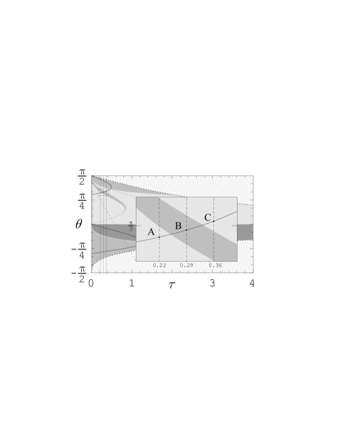
Figure 7: Parameter-induced macroscopic change in the stability of the trimer dynamics. The figure shows the magnification of a portion of the upper half plane of the non-dimeric stability diagram, figure 4, along with the non-dimeric $\tau$-curve (see (15), (25)) relevant to $\nu=0$ (solid) and the straight lines corresponding to three different choices of the hopping parameter, $\tau_{\rm A}$, $\tau_{\rm B}$ and $\tau_{\rm C}$ (dashed). The ensuing intersections are denoted A, B and C, respectively. Notice that B belongs to the narrow unstable region (which we term isthmus), whereas A and C belong to the wide stable region surrounding it. The changes in the stability character of the fixed point resulting from such a relatively slight increase of $\tau$ are evident in figure 8.

The first and last choice –corresponding to trajectories based in the neighborhood of a stable fixed point– are both characterized by extremely regular sections where the populations “flicker” about their initial configuration. In the remaining case, the fixed point belongs to the “unstable isthmus” (see figure 7), and the consequent irregular trajectories produce a quite different pattern. Also in the present case, a slight change in the parameters destroys the steady, flickering populations. Once again the Poincaré sections are indistinguishable from one another and densely fill an area considerably larger than in the previous cases.

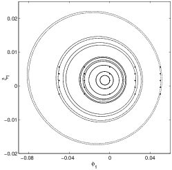
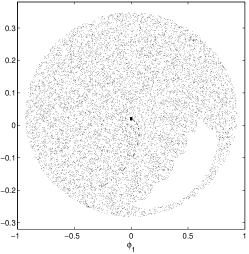
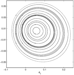
Figure 8: Poincaré sections of trajectories based in the vicinity of the configurations A, B, C selected in figure 7. In every case one of the lateral condensates is almost empty, whereas the other two share almost equally the remaining boson population, which adds up to more than 97% of the total. The phases of the macroscopically filled condensates are parallel to each other and opposite to that of the almost empty condensate [such configurations are close to the reduced-phase-space point $(\phi_{1},\xi_{1},\phi_{2},\xi_{2})=(0,0.016,\pi,-0.984)$]. The three situations are distinguished by (from left to right) $\tau=0.22$, $\tau=0.29$, $\tau=0.36$; in every instance $\nu=0$. The features of the Poincaré sections clearly mirror the stability character of the relevant fixed points. Notice furthermore that the central Poincaré section, relevant to the choice falling in the unstable “isthmus” of figure 7, covers a region roughly an order of magnitude wider than the lateral sections, relevant to stable regions.

4.3 Instability suppression due to fixed-point disappearance

So far, we have examined two situations where the change in the phase-space structure is associated with a modification in the stability character of a fixed point. Nevertheless, such a change may be also related to the disappearance of a fixed point. When $\nu=0.52$, e. g., a consistent portion of the lower branch of the non-dimeric $\tau$-curve falls in the forbidden zone, similar to the curve featuring the narrowest dashing style in figure 4. However, for $\tau=1.66$ (i.e. very close to the branch tip), both of the solutions associated to the lower branch are acceptable. According to the stability diagram, one of them is a maximum, whereas the other is an unstable saddle. Actually, the trajectories in the neighborhood of this configuration, produce the expected irregular Poincaré sections, displayed in the central panel of figure 9. As $\tau$ is decreased, the unstable solution moves toward the forbidden zone (see figure 4). For $\tau=1.5$, the maximum is the only non-dimeric fixed point surviving. The change in the phase-space structure associated to the disappearance of the unstable fixed point is quite evident in the leftmost panel of figure 9 that shows the Poincaré sections obtained from the same set of base points considered in the case $\tau=1.66$. Despite some features signalling a certain degree of chaoticity, the sections are much more regular and can be easily distinguished from each other. The unstable fixed point, as well as the stable one, disappears also if $\tau$ is increased by a sufficient amount (the disappearance of fixed points takes place at the branch tip after a coalescence process). Similar to the previously examined situation, an increase in the regularity of the Poincaré sections is observed for $\tau=1.82$, when only dimeric fixed points are present (rightmost panel of figure 9).

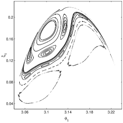
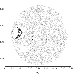
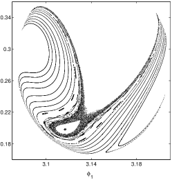
Figure 9: Regularization of the phase-space due to the disappearance of an unstable fixed point. All of the three sets of Poincaré sections refer to $\nu=0.52$, and have been obtained from trajectories based in the vicinity of the same configuration. For $\tau=1.66$ such configuration is an unstable saddle, and produces quite irregular trajectories, as shown in the central panel. Slight variations of the hopping amplitude cause the disappearance of the unstable fixed point, and this in turn results in an increase in the regularity of the trajectories based in the vicinity of the corresponding configuration (see discussion in section 4.3). This is clearly visible in the leftmost and rightmost panels of the figure, pertaining to $\tau=1.5$ and $\tau=1.82$, respectively.

5 Phase-triggered population oscillations near the CDW configuration

The last case considers several unexpected and interesting features of CDW fixed points. Remarkably, these fixed points are always present independently from the value of the parameters $\tau$ and $\nu$, and have a simple configuration where the entire boson population is equally shared between the lateral condensates, being the phases opposite to each other. Figure 5 shows that the CDW are saddle points and are expected to exhibit a stable character in extended regions of the parameter plane. This fact, is widely confirmed by our numeric simulations where, for initial configurations sufficiently close to the CDW fixed point, we observe a regular dynamics exhibiting (possibly quite complex) periodic oscillations of the three condensate populations. In particular, the lateral condensates cyclically exchange small amounts of bosons, so that their population imbalance oscillates. Whereas the central condensate, whose population oscillates with a considerably smaller amplitude and a frequency twice than that of the lateral condensates, participates in the dynamics acting as a bridge between the lateral ones.

Figure 10 shows the evolution of a configuration quite close to the CDW for two parameter choices belonging to different stability regions of figure 5.

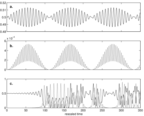
Figure 10: Evolution of an initial configuration slightly displaced from the CDW, ${\bf z}=(1/2,0,1/2e^{i(\pi-\varphi)})$, $\varphi=5\cdot 10^{-3}$. Black and grey solid lines represent $n_{1}/N$ and $n_{2}/N$, respectively. Panels a and b refer to the parameter choice $\nu=0$, $\tau=0.703$, belonging to a stable region but very close to the border dividing it from an unstable region (see figure 5 and (27)). The evolution displayed in panel c was obtained increasing $\tau$ by 0.005. This was sufficient to cross the border and enter the unstable region. The predicted instability of the CDW is confirmed by the strongly irregular character of the dynamics, which fully shows up after an apparently regular transient. The remaining population, $n_{3}$, (not shown) can be found exploiting the conservation of the total number of bosons $\sum_{j}n_{j}=N$. In the regular case, panels a and b, it essentially balances the oscillations of $n_{1}$, $n_{2}$ being almost vanishing.

As expected, in the stable case (panels a and b), the amplitude of the population oscillations increases with increasing displacement of the initial configuration from the CDW. Of course, in general, such displacement cannot be increased indefinitely: the initial configuration would eventually leave the “domain of influence” of the CDW and the consequent trajectory would be determined by the stability character of a different fixed point. The same considerations apply to configurations obtained from the CDW by setting the phase difference between the lateral condensates to a value $\theta_{31}=|\theta_{3}-\theta_{1}|\neq\pi$ and maintaining the total boson population equally shared by the lateral condensates. In this case the oscillation amplitude is a function of $|\theta_{3}-\theta_{1}|$ with a minimum at $|\theta_{31}|=\pi$, where it vanishes. Our numeric simulations confirm these predictions. In fact, for sufficiently small $\tau$’s, regular oscillatory dynamics is observed over the entire range of $\theta_{31}$. This is clearly shown in figure 11, displaying the population oscillations pertaining to initial configurations identified by several values of $\theta_{31}$.

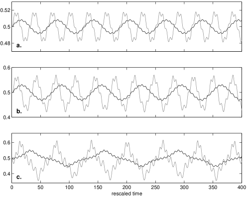
Figure 11: Oscillation of the population $n_{1}$ relevant to initial configurations where the total number of bosons is equally shared by the lateral condensates. The three panels refer to different (increasing) values of the phase difference $\theta_{31}=|\theta_{3}-\theta_{1}|$. a. $\theta_{31}=9/10\pi$; b. $\theta_{31}=1/2\pi$; c. $\theta_{31}=1/10\pi$. Black and grey lines refer to $\tau=0.1$ and $\tau=0.2$, respectively. In every case there was no bias on the central condensate ($\nu=0$). Notice that the oscillation amplitude increases with increasing $\theta_{31}$. Notice also the incipient anharmonic shape of the oscillations for small $\theta_{31}$ (panel c.)

A further important feature of the CDW fixed points is highlighted by figure 12 showing that for small values of $\tau$, the amplitude $a_{1}$ of the oscillation of the population $n_{1}$ exhibits a quite simple dependence on the phase difference $\theta_{31}$ of the relevant initial configuration. More precisely $a_{1}$ linearly depends on $\cos(\theta_{31}/2)$. A rigorous discussion of such dependence is beyond the scope of the present article. However, some insight in this sense can be gained by adopting an approach similar to that developed in  [47] in the study of the stability of the dimeric integrable subregime.

Figure 12: Amplitude of the population oscillations of one of the lateral condensates for different values of the initial phase difference $\theta_{31}$ and $\nu=0$. Crosses ($\times$): $\tau=0.1$; Plus signs ($+$): $\tau=0.15$. The straight lines are linear fits of the two sets of data.

Interestingly, the same linear behavior as in figure 12 is obtained by relaxing the requirement that the entire boson population is equally shared by the two lateral condensates. This is clearly shown in figure 13, where we plotted the average oscillation amplitude relevant to initial configurations characterized by a certain phase difference $\theta_{31}$ and condensate populations $n_{j}$ slightly displaced from that of the CDW fixed point.

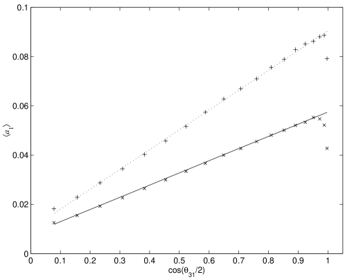
Figure 13: A simple dependence of the population oscillation on the initial phase difference $\theta_{31}$ is present even if the initial population configuration does not reproduce that of the CDW exactly. Each of the plotted data was obtained averaging the results of 300 simulations where the initial populations were allowed to differ by about 1% from the configuration $(1/2,0,1/2)$, and the phase of the central (almost depleted) condensate was chosen randomly.

The plots displayed in figures 12 and 13 suggest the possibility of measuring the phase difference between two equally populated condensates. Let us stressing the fact that, in order to profitably exploit this quantum effect to measure the difference of phase between two condensates, we need of a nondestructive real-time probing of the condensates such as the technique employed to image dimer-like condensates confined by magnetic traps [49, 50].

6 Conclusions

The present paper has been inspired by the wish of gaining a deeper insight both on the complexity of three-well dynamics (which, as noted above, is the paradigm of the behavior one can expect in more complex BECs arrays) and on the possibility of detecting macroscopic effects amenable to experimental observation.

Recently, it has been proposed that the superposition of multiple laser beams could allow to create unusual optical lattices in a controlled manner [51]. In this respect, we observe that a suitable choice of laser wavelengths could generate a superlattice whose elementary cell is characterized by a three-well potential such as the one addressed in the present paper. The further minimization of the tunneling between subsequent trimeric cells should provide an alternative experimental realization of the system under concern. A nice example in this sense is the trimerized Kagomè optical lattice [52] providing (multiple copies of) the trapping potential typical of a symmetric closed trimer.

In the present paper we focus on the rich phenomenology offered by the trimer and on the possibility of triggering macroscopic effects through a suitable choice of the adjustable parameters, relegating as much as possible to the appendices the technical details necessarily involved in a systematic analysis. The macroscopic effects we evidence in this paper are obtained through a careful analysis of the stability diagrams introduced in [39], whose operational value is reviewed in section 3. Their derivation is thoroughly discussed in A. Such diagrams describe the trimer phase space in terms of the stability character of dynamical fixed points for any choice of the significant parameters. This wealth of information enriches the recent literature about the dynamical stability of mesoscopic BEC arrays [19]-[21], [25]-[29], [53] and supplies an essential tool in designing experimental realizations of the trimer dynamics. Also, at the theoretical level, it provides a sound basis for gaining a deeper insight into the quantum counterpart of classical dynamical instability, which is far from being fully understood.

The use of stability diagrams leads to identify in section 4 three different mechanisms able to modify in a substantial way the trimer dynamics. These are exploited in sections 4.1, 4.2 and 4.3 to prime instability in breather-like regular oscillations, loss of coherence in anti-breather states, and suppression of instability due to fixed-point disappearance, respectively. Macroscopic dynamical oscillations are shown to be triggered by means of slight parameter changes thus providing a stimulating basis for planning actual experiments in the scheme described in [4]-[8]. The analysis of the stability diagrams in section 5 also evidences that a simple configuration exists allowing to relate in a direct manner the initial phase difference between two condensates to the amplitude of the ensuing population oscillations. This suggests a rather simple scheme aimed at testing experimentally the limits of validity of the mean-field picture, where each condensate is endowed with a macroscopic phase. The study of the fixed points –inherent in the classical picture– reported in sections 2 and 3 proves useful also in unraveling the complex structure of the energy spectrum of the quantum trimer, in that it allows to recognize a (either exact or approximate) mapping with a simpler dimeric system [54]. The mapping is shown to persist also at the quantum level, thus extending the results found in [24] to the case of the quantum trimer. These results provide a useful starting point in investigating the quantum counterpart [33] of classical dynamical instability. A deeper insight into the relation between the classical and quantum picture is certainly useful for the approaches to this issue based on the dynamical algebra method [13, 42, 47] or on the measure of quantum-state entanglement [55].

Appendix A Derivation of the stability diagrams

The linear stability character of a fixed point ${\mathbf{x}}^{t}=(x_{1},x_{2},x_{3})$ can be determined by studying the eigenvalues of the matrix associated to the (linearized) equations governing the dynamics of the (small) displacements ${\mathbf{v}}^{t}=({\mathbf{q}}^{t},{\mathbf{p}}^{t})$ from the fixed point itself, where ${\mathbf{z}}^{t}=(z_{1},z_{2},z_{3})=\sqrt{N}({\mathbf{x}}+{\mathbf{q}}^{t}+i\,{\mathbf{p}}^{t})$. The Hamiltonian, up to the second order in the small displacements ${\mathbf{v}}^{t}$, reads

$${\cal H}({\mathbf{z}})-\chi N={\cal H}(\sqrt{N}{\mathbf{x}})+UN^{2}\frac{\tau}{2}{\mathbf{v}}^{t}M_{h}{\mathbf{v}},$$ (17)

where

$$M_{h}=\left(\begin{array}[]{cc}Q&0\\ 0&P\end{array}\right),\,\,\,Q=\left|P_{hk}+\frac{8x_{j}^{2}}{\tau}\delta_{hk}\right|,\,\,\,P=\left(\begin{array}[]{ccc}\Delta_{1}&-1&0\\ -1&\Delta_{2}&-1\\ 0&-1&\Delta_{3}\end{array}\right)$$ (18)

and $\Delta_{j}=2(2x_{j}^{2}-m-\delta_{j\,2}\,\nu)/\tau$. As it is well known, linear instability occurs when at least one of such (in principle complex) eigenvalues features a positive real part. The linearized equations obtained from Hamiltonian (17) through Poisson’s brackets $\{q_{j},p_{k}\}=\,\frac{\delta_{jk}}{2\,N\,\hbar}$ (these stem from the original ones $\{z_{j},z^{*}_{k}\}=\frac{i\delta_{jk}}{\hbar}$) have the form

$$\dot{\mathbf{v}}=\{{\mathbf{v}},{\cal H}\}=\frac{U\,N\,\tau}{2\,\hbar}M_{s}{\mathbf{v}},\qquad M_{s}=\left(\begin{array}[]{cc}0&Q\\ -P&0\end{array}\right).$$ (19)

In accordance with the expected time reversal symmetry of the linear dynamics, the six (complex) eigenvalues of matrix $M_{s}$ come in pairs featuring the same modulus and opposite signs. More precisely each pair of eigenvalues of $M_{s}$ consists in the signed square roots of an eigenvalue of the three-by-three matrix $-QP$. Indeed, due to the diagonal block structure of $M_{s}$, the relevant eigenvalue equation is ${\cal D}(\lambda)=\det(\lambda I-M_{s})=\det(\lambda^{2}I+QP)=\lambda^{2}(\lambda^{4}-s\lambda^{2}+p)=0$, where in writing the characteristic polynomial of $-QP$ we took into account the fact that, similar to $P$, such a matrix has a zero eigenvalue. This feature is the consequence of the fact that both ${\mathbf{q}}^{t}$ and ${\mathbf{p}}^{t}$ are constrained by the condition $|z_{1}|^{2}+|z_{2}|^{2}+|z_{3}|^{2}=N$. According to ${\cal D}(\lambda)=0$ the fixed point is (linearly) stable provided that the three conditions

$$s^{2}-4p\geq 0,\qquad s\leq 0,\qquad p\geq 0$$ (20)

are simultaneously met. Indeed in this case the two non-zero eigenvalues of $-QP$ are real and non-positive, so that the four non-zero eigenvalues of $M_{s}$ — namely their signed square roots — are purely imaginary. Conversely, whenever an eigenvalue of $-QP$ is complex or real positive, one of its square roots has necessarily a positive real part, giving rise to (linear) instability. The following subsections describe in some detail the construction of the stability diagrams for the DFP, the NFP and the CDW.

A.1 Dimeric fixed points

As illustrated in section 2, the dimeric fixed points (DFP) pertain to the integrable dimeric subregime [47] of the dynamics described by system (3), which is characterized by $z_{1}(t)\equiv z_{3}(t)$. In this situation the fixed point configuration $(x_{1},x_{2},x_{3})$ is described by $x_{1}(\theta)=x_{3}(\theta)=\cos\theta/{\sqrt{2}}$ and $x_{2}(\theta)=\sin\theta$ (see Eqs. (8)), where the tangent ${\alpha}(\theta)=\tan(\theta)={x_{2}}/({\sqrt{2}\,x_{1}})$ must be a real root of polynomial ${\cal P}({\alpha};\tau,\nu)\equiv{\alpha}^{4}+A_{\nu}\tau^{-1}{\alpha}^{3}-B_{\nu}\tau^{-1}{\alpha}-1$ (see formula (9)) with $A_{\nu}=\sqrt{2}(2-\nu)$, $B_{\nu}=\sqrt{2}(1+\nu)$. Before proceeding to a more detailed discussion of the DFP case, we remark that the previous polar representation of $x_{j}$’s allows one to readily relate variable $\theta$ to the fixed point $(x_{1},x_{2},x_{3})$. Particularly, $\tan(\theta)={x_{2}}/({\sqrt{2}\,x_{1}})$ shows how $\theta\approx 0$ corresponds to a situation where the central condensate is almost depleted, so that the total population is (equally) shared by the lateral condensates. Conversely, when $\theta\approx\pm{\frac{\pi}{2}}_{\mp}$ the lateral condensates are almost empty and the total population is concentrated in the central one. Notice also that the sign of $\theta$ is similarly strictly related to the phase differences between the central condensate and the lateral ones. More precisely such phase differences are 0 or $\pm\pi$ depending on whether $\theta$ is positive or negative.

As we discussed above, solving the fixed point equations for the DFP amounts to finding the real roots of the fourth-degree polynomial ${\cal P}({\alpha};\tau,\nu)$ (henceforth denoted by $P_{D}({\alpha};\tau;\nu)$). Four real solutions are found from $P_{D}({\alpha};\tau;\nu)=0$ for

$$\left|\nu-{1}/{2}\right|<\,{1}/{2},\quad\tau\leq\frac{1}{\sqrt{2}}\left[\left({3}/{2}\right)^{{2}/{3}}-\left|\nu-{1}/{2}\right|^{{2}/{3}}\right]^{{3}/{2}}$$ (21)

and two real solutions elsewhere in the parameter plane, as it is illustrated in figure 1. In section 3, we showed how equation $P_{D}({\alpha};\tau;\nu)=0$ suggests that, for any choice of parameters $\tau=\tilde{\tau}$, $\nu=\tilde{\nu}$, the DFP can be found in the $\theta-\tau$ plane from the intersection of the parametric curve (see 15)

$$\tau=\tau_{D}({\alpha};\nu)=\sqrt{2}\,{\alpha}\,\frac{(\nu-2){\alpha}^{2}+(\nu+1)}{{\alpha}^{4}-1}\,,\quad\nu=\tilde{\nu}\,,$$ (22)

with the vertical straight line $\tau=\tilde{\tau}$. The curve $\tau_{D}(\alpha;\tilde{\nu})$ features two asymptotes at $\theta=\pm\pi/4$ (${\alpha}=\pm 1$). This is in agreement with the fact that polynomial $P_{D}({\alpha};\tau,\nu)$ has no less than two real solutions. In particular it is easy to verify that when $\nu=1/2$ the values $\theta=\pm 1/2$ are solutions of $P_{D}({\alpha};\tau;\nu)=0$. Hence, in this case, the two unbounded branches coalesce with their asymptotes, thus providing $\tau$-independent solutions corresponding to the configurations $(x_{1},x_{2},x_{3})=(1/2,\pm 1/\sqrt{2},1/2)$. More generally, when $\nu\neq 1/2$ the branches of the curve $\tau_{D}(\alpha;\tilde{\nu})$, and hence the roots of $P_{D}({\alpha};\tau;\nu)=0$, are characterized by a reflection symmetry with respect to the nearest asymptote (see figure 2). This can be seen by noticing that

$$\tau_{D}\left[\tan\left(\vartheta\pm\frac{\pi}{4}\right);\bar{\nu}+\frac{1}{2}\right]=\frac{2\,\bar{\nu}\mp 3\sin(2\vartheta)}{\sin(2\vartheta)}\frac{\cos(2\vartheta)}{2\sqrt{2}}\,,\,\vartheta\in\left[-\frac{\pi}{4},\frac{\pi}{4}\right]$$ (23)

where the auxiliary angle $\vartheta$ describes the positive (negative) solutions $\theta=\vartheta+\pi/4$ ($\theta=\vartheta-\pi/4$). One easily verifies that $\tau_{D}\bigl{[}\tan(\vartheta\pm{\pi}/{4});\bar{\nu}+{1}/{2}\bigr{]}=\tau_{D}\bigl{[}\tan(\pm{\pi}/{4}-\vartheta);{1}/{2}-\bar{\nu}\bigr{]}$.

Local character of the DFP. This information is obtained by exploiting the constraint $x_{j}\neq 0$ and the fixed point equations (6). After expressing the quantities appearing in matrices $Q$ and $P$ (see (18)) as $\Delta_{1}=\Delta_{3}={x_{2}}/{x_{1}}=\sqrt{2}\,{\alpha}$ and $\Delta_{2}=(x_{1}+x_{3})/{x_{2}}={\sqrt{2}}/{\alpha}$, the analysis of the signature of both matrix $Q$ and $P$ depending on parameter $\alpha=\tan\theta$ leads to the following conclusions. For any choice of the parameters $\tau$ and $\nu$, a DFP is a minimum if the corresponding angular coordinate, $\theta$, is positive. If, conversely, $\theta<0$ the fixed point is either a maximum or a saddle point depending on whether $\tau$ is greater or less than $d(\tan\theta)$ where $d({\alpha})=\max\left[d_{1}({\alpha}),d_{2}({\alpha})\right]$ with $d_{1}({\alpha})=-2{\sqrt{2}}/[\alpha(1+{\alpha}^{2})]$ and $d_{2}({\alpha})=$ $-6{\sqrt{2}}/[\alpha^{3}(1+{\alpha}^{2})^{3}]$. Combining such results with the linear stability analysis based on equation ${\cal D}(\lambda)=0$ (defined after formula (19)) confirms that both maxima and minima are, as expected, stable fixed points, whereas all the saddles of the dimeric regime are unstable. The situation for the DFP is summarized in the corresponding stability diagram displayed in figure 2. The differently shaded region pertain to fixed points with a different stability character.

A.2 Non dimeric regime

Since in this case $x_{1}\neq x_{3}$, the polar representation of nondimeric fixed points (NFP) is not as simple as that of the DFP case. Still, one can take advantage from the conservation of the total boson number. Some algebraic manipulations of the fixed-point equations (see non-dimeric solutions in section 2.1) suggest to switch to the new coordinates $X_{1}=$ $(x_{1}+x_{3})/\sqrt{2}$, $X_{2}=x_{2}$ and $X_{3}=(x_{1}-x_{3})/{\sqrt{2}}$, obeying the constraint $X^{2}_{1}+X^{2}_{2}+X^{2}_{3}=1$, before setting $X_{1}=R\cos\theta$ and $X_{2}=R\sin\theta$. This way $X_{3}=\pm\sqrt{1-X_{1}^{2}-x_{2}^{2}}$ and radial coordinate (11) are shown to depend on $\theta$ and $\tau$ as

$$R({\alpha};\,\tau)=\sqrt{\frac{(1+\alpha^{2})(2\sqrt{2}-\alpha\,\tau)}{2\sqrt{2}(2+\alpha^{2})}},\,X_{3}(\alpha)\!=\pm\sqrt{\frac{4\!+\!\sqrt{2}\alpha(1+\tau\alpha^{2})}{4(2+{\alpha}^{2})}}$$ (24)

with ${\alpha}=\tan\theta={X_{2}}/{X_{1}}$, and the fixed points equations are equivalent to the equation for the roots of polynomial ${\cal P}({\alpha};\tau,\nu)\equiv{\alpha}^{4}+A_{\nu}\tau^{-1}{\alpha}^{3}-B_{\nu}\tau^{-1}{\alpha}-{4}/{3}=0$, (henceforth denoted by $P_{N}({\alpha};\nu,\tau)$), where $A_{\nu}={2\sqrt{2}(2-\nu)}/{3}$, $B_{\nu}={4\sqrt{2}(1+\nu)}/{3}$ (see 12). Recalling that we are ultimately looking for real solutions of system (6) it is clear that the roots which make $R({\alpha})$ or $X_{3}(\alpha)$ imaginary must be discarded. Before analysing how NFP are identified, it is important to remark that in the NFP case the relation among the auxiliary variable $\theta$ and the configuration of the fixed point is not as transparent as in the DFP case, basically due to the $\theta$ dependence of the radial variable (24). Nevertheless, within the NFP stability diagram some special regions can be still recognized. Notice indeed that, according to the previous definitions of $X_{1}$, $X_{2}$ and $X_{3}$ as well as to (24), the (forbidden) limit situations $X_{3}\to 0$ and $R\to 0$ correspond to the dimeric case $x_{1}=x_{3}$ and to the CDW case $x_{1}=-x_{3}$, $x_{2}=0$, respectively. As we shall discuss below, these limit situations are actually the boundaries of two forbidden regions in the NFP diagram (see (26) and discussion). Due to the restrictions on $R$ and $X_{3}$, the diagram of figure 3, giving the number of fixed points relevant to system (6) on varying parameters $\tau$ and $\nu$, is significantly richer than the corresponding diagram for the number of real roots of polynomial $P_{N}({\alpha};\nu,\tau)$. Indeed the latter consists of four regions, delimited by the solid lines appearing in figure 3. Two of these regions correspond to situations where $P_{N}({\alpha};\nu,\tau)$ features only two real roots, whereas within the remaining regions the roots are either four or none. Despite they are real, some of these roots can make either $R({\alpha})$ or $X_{3}({\alpha})$ complex. Hence some new regions appear within the ones delimited by the solid curves, where the number of solutions must be decreased by either one or two units.

As discussed in section 3, the features of diagram (3) can be better understood by resorting to the $\theta-\tau$ plane, where, similar to the DFP case, for a given choice $\tau=\tilde{\tau}$, $\nu=\tilde{\nu}$, the real roots of polynomial $P_{N}({\alpha};\nu,\tau)$ correspond to the intersections of curve

$$\tau_{N}({\alpha};\nu)=2\,{\alpha}\,[(\nu-2){\alpha}^{2}+\nu+2]/(3{\alpha}^{4}+1)\,,\quad\nu=\tilde{\nu}\,,$$ (25)

with the straight line $\tau=\tilde{\tau}$. In the half plane $\tau>0$ such curve consists in general of two bounded, roughly bell-shaped, branches. More precisely they are defined within the $\theta$ intervals $[-\nu_{b},0]$ and $[\nu_{b},\pi/2]$, respectively, where $\nu_{b}=$ $\arctan(\sqrt{(2+\nu)/(2-\nu)})$. When $\nu>2$ ($\nu<-2$) the former (latter) branch, which from now on will be referred to as the negative (positive) branch, disappears. These features readily explain the four regions in the diagram describing the number of real roots of $P_{N}({\alpha};\nu,\tau)$. Hence, provided $\tilde{\tau}$ is sufficiently small, there are either four or two solutions depending on whether $|\tilde{\nu}|<2$ or $|\tilde{\nu}|>2$. Indeed, for any straight line at a given value of $\tau$, there exist for each branch a value of $\nu$ such that the branch and the straight line are tangent. Denoting such values $\bar{\nu}_{t}^{\pm}(\tau)$, where the superscript labels the branch, it is easy to check that $\mp\bar{\nu}_{t}^{\pm}(\tau)$ is always a growing function of $\tau$. Hence two solutions relevant to the negative (positive) branch are always present for $\nu>\bar{\nu}_{t}^{-}(\tau)$ [$\nu<\bar{\nu}_{t}^{+}(\tau)$]. Notice further that the presence of a region of parameters where four solutions are found implies that there exists some $\tau_{c}>0$ such that $\bar{\nu}_{t}^{+}(\tau_{c})=\bar{\nu}_{t}^{-}(\tau_{c})$. Then it is clear that $P_{N}({\alpha};\nu,\tau)$ features four real roots in the region $\{\bar{\nu}_{t}^{-}<\nu<\bar{\nu}_{t}^{+};\,\tau<\tau_{c}\}$, no real roots in the region $\{\bar{\nu}_{t}^{+}<\nu<\bar{\nu}_{t}^{-};\,\tau>\tau_{c}\}$ and two real roots elsewhere. The explicit expressions of functions $\bar{\nu}_{t}^{-}(\tau)$ and $\bar{\nu}_{t}^{+}(\tau)$ for ${\alpha}<0$ and ${\alpha}>0$, respectively, (solid lines in figure 4) can be easily described in a parametric way by means of two curves $\tau_{t}({\alpha})$, $\nu_{t}({\alpha})$: the curve $\tau_{t}({\alpha})=16\,{\alpha}^{3}/(3{\alpha}^{6}+9{\alpha}^{4}-3{\alpha}^{2}-1)$ intersects $\tau_{N}({\alpha};\nu)$ at the tips of its bell-shaped branches while $\nu_{t}(\alpha)$ is such that $\frac{d}{d{\alpha}}\tau_{N}({\alpha};\nu)=0$ at ${\nu=\nu_{t}({\alpha})}$ and $\tau_{N}[{\alpha};\nu_{t}({\alpha})]=\tau_{t}({\alpha})$. The requirement that $R$, $X_{3}\in{\mathbb{R}}$ determines two forbidden regions in the stability diagram:$\{\theta<0,\;\tau>\tau_{3}(\tan\theta)\}$ and $\{\theta>0,\;\tau>\tau_{R}(\tan\theta)\}$, where

$$\tau_{3}({\alpha})=-{2}/{{\alpha}(1+2\,{\alpha}^{2})},\qquad\tau_{R}({\alpha})={2}/{\alpha}\,,$$ (26)

(see figure 4). The information about the forbidden regions can be visualized in parallel in the $\tau\!-\!\nu$ plane by drawing the curves $\bar{\nu}_{R}(\tau)$ and $\bar{\nu}_{3}(\tau)$ describing the intersections between $\tau_{N}(\alpha;\nu)$ and the borders of the forbidden regions, $\tau_{R}({\alpha})$ and $\tau_{3}({\alpha})$, respectively (dotted curves of figure 3). According to what we said so far, these curves enclose two regions where one of the real roots of polynomial $P_{N}({\alpha};\nu,\tau)$ must be excluded from the set of solutions of system (6): $\nu>\bar{\nu}_{3}(\tau)$ and $\nu<\bar{\nu}_{R}(\tau)$. Similarly two of these real roots must be discarded in the regions $\{\bar{\tau}_{R}(\nu)<\tau<\tau_{t}^{+}(\nu),\,\nu<\nu_{2}^{+}\}$ and $\{\bar{\tau}_{3}(\nu)<\tau<\tau_{t}^{-}(\nu),\,\nu>\nu_{2}^{-}\}$. Notice also that $\tau_{R}(\nu)$ [$\tau_{3}(\nu)$] is expectedly tangent to $\bar{\nu}_{t}^{+}(\tau)$ [$\bar{\nu}_{t}^{-}(\tau)$] at $\tau=\tau_{2}^{+}$, [$\tau=\tau_{2}^{+}$].

Local character of the NFP. The study of the signature of both matrix $Q$ and $P$ defined in (18) reveals that NFPs are either maxima or saddle points depending on whether they lie within the region $\{\theta<0,\,\tau_{t}(\tan\theta)<\tau<\tau_{3}(\tan\theta)\}$ or elsewhere in the allowed zone. In parallel, the linear stability analysis based on polynomial ${\cal D}(\lambda)$ (see the discussion relevant to (20)) discloses the (linear) stability of most of the saddle points lying in the positive $\theta$ quadrant, namely the ones belonging to the light grey region of figure 4. Indeed, within the allowed region $\{\theta<0,\,\tau<\tau_{3}(\tan\theta)\}\cup\{\theta>0,\,\tau<\tau_{R}(\tan\theta)\}$, the stability condition (20) fails to apply in the region $\{\theta<0;\,\tau<\tau_{t}(\tan\theta)\}\cup\{\theta>0;\,\tau>\tau_{t}(\tan\theta)\}$, where $p<0$, and in a peculiarly shaped region of the positive $\theta$ quadrant, where $s^{2}-4p<0$. Since $s$ is positive everywhere outside these regions, it turns out that linear stability characterizes not only, as expected, the maxima, but also most of the saddle points at positive $\theta$.

A.3 Central depleted well

As discussed in section 2, there is only one parameter-independent CDW fixed point: ${\mathbf{x}}=(1/\sqrt{2},0,-1/\sqrt{2})$, which, according to the signature of matrices $Q$ and $P$ (see 18), is always a saddle point. Indeed, no matter for the sign of $\Delta_{2}=-2\,(1+\nu)/\tau$, the quadratic form has always an undefined signature. Recalling that $\Delta_{1}=\Delta_{3}=0$, the coefficients involved stability condition (20) have the quite simple form $s=4[\tau^{2}+(1+\nu)^{2}]/{\tau^{2}}$ and $p=4[\tau^{2}+4(1+\nu)]/{\tau^{2}}$ yielding $\Delta=16\,\left[2\,(\nu^{2}-1)\tau^{2}+(\nu+1)^{4}\right]/\tau^{4}$. Hence, introducing the functions

$$c_{1}(\nu)=2\,\sqrt{-1-\nu},\qquad c_{2}(\nu)=\sqrt{(1+\nu)^{3}/[2\,(1-\nu)]}$$ (27)

the CDW saddle is actually stable in the parameter regions $\{\tau>c_{1}(\nu);\,\nu<-1\}$, $\{\tau<c_{2}(\nu);\,|\nu|<1\}$ and $\{\tau>0;\,\nu>1\}$, and unstable elsewhere. Notice that the former zone can be also described as $\nu<\bar{\nu}_{R}(\tau)$, where $\nu_{R}$ is strictly related to the boundary of one of the forbidden zones of the NFP stability diagram. Actually, as we already noticed above, the points lying on such (forbidden) boundary $\tau=\tau_{R}(\tan\theta)$ have a CDW form, since $R({\alpha};\,\tau)=0$ there (see (26) and the defining formulas for $X_{j}=X_{j}(R,\theta)$, $j=\,1,2,3$ in section A.2). The stability diagram for the CDW fixed point is displayed in figure 5. Notice that, unlike figures 2 and 4, it is in the plane of the parameters, $\tau$ and $\nu$. This is possible because, as we already remarked, there is always a single, parameter-independent CDW configuration.

References

References

- [1] Burger S, Cataliotti F S, Fort C, Minardi F, and Inguscio M 2001 Phys. Rev. Lett. 86, 4447
- [2] Cataliotti F S, Burger S, Fort C, Maddaloni P, Minardi F, Trombettoni A, Smerzi A, and Inguscio M 2001 Science 293, 843
- [3] Öttl A, Ritter S, Köhl M, and Esslinger T 2005 Phys. Rev. Lett. 95, 090404
- [4] Anker Th, Albiez M, Gati R, Hunsmann S, Eiermann B, Trombettoni A, and Oberthaler M K 2005 Phys. Rev. Lett. 94, 020403
- [5] Albiez M, Gati R, Fölling J, Hunsmann S, Cristiani M, and Oberthaler M K 2005 Phys. Rev. Lett. 95, 010402
- [6] Gati R, Albiez M, Fölling J, Hemmerling B, and Oberthaler M K 2006 App. Phys. B 82, 207
- [7] Gati R, Esteve J, Hemmerling B, Ottenstein T B, Appmeier J, Weller A, and Oberthaler M K 2006 N. J. Phys. 8, 189
- [8] Gati R, and Oberthaler M K 2007 J. Phys. B 40, R61
- [9] Smerzi A, Fantoni S, Giovanazzi S, and Shenoy S 1997 Phys. Rev. Lett. 79, 4950
- [10] Milburn G J, Corney J, Wright E M, and Walls D F 1997 Phys. Rev. A 55, 4318
- [11] Menotti C, Anglin J R, Cirac J I, and Zoller P 2001 Phys. Rev. A 63, 023601
- [12] Franzosi R, Penna V, and Zecchina R 2000 Int. J. Mod. Phys. B 14, 943
- [13] Franzosi R and Penna V 2001 Phys. Rev. A 63, 043609
- [14] Nemoto K, Holmes C A, Milburn G J and Munro W J 2001 Phys. Rev. A 63, 013604
- [15] Franzosi R and Penna V 2002 Phys. Rev. A 65, 013601
- [16] Jaksch D, Bruder C, Cirac J I, Gardiner C W, and Zoller P 1998 Phys. Rev. Lett. 81, 3108
- [17] Polkovnikov A, Sachdev S, and Girvin S M 2002 Phys. Rev. A 66 053607
- [18] Oelkers N, and Links J 2007 Phys. Rev. B 75 115119
- [19] Wu B, and Niu Q 2001 Phys. Rev. A 64, 061603(R)
- [20] Paraoanu G S 2003 Phys. Rev. A 67, 023607
- [21] Kalosakas G, Rasmussen M, and Bishop A R 2002 Phys. Rev. Lett. 89, 030402
- [22] Raghavan S, Smerzi A, Fantoni S, and Shenoy S 1999 Phys. Rev. A 59, 620
- [23] Giovanazzi S, Smerzi A, and Fantoni S 2000 Phys. Rev. Lett. 84, 004521
- [24] Aubry S, Flach S, Kladko K, and Olbrich E 1996 Phys. Rev. Lett. 76, 1607
- [25] Franzosi R, and Penna V 2003 Phys. Rev. E 67, 046227
- [26] Stickney J A, Anderson D Z, and Zozulya A A 2007 Phys. Rev. A 75 013608
- [27] Liu B, Fu L-B 2007 Phys. Rev. A 75, 033601
-
[28]
Pando C L and Doedel E J 2007 Phys. Rev. E 75, 016213
Pando C L and Doedel E J 2005 Phys. Rev. E 71 056201 - [29] Chong G, Hai W, and Xie Q 2005 Phys. Rev. E 71, 016202
- [30] Kolovsky A R, Korsch H J and Graefe E M arXiv: 0901.4719v1 quant-ph
- [31] Nemoto K, Sanders B C 2001 J. Phys. A: Math. Gen. 34 2051
- [32] Mossmann S and Jung C 2006 Phys. Rev. A 74 033601
- [33] Kolovsky A 2007 Phys. Rev. Lett. 99, 020401
- [34] Hiller M, Kottos T, and Geisel T 2006 Phys. Rev. A 73, 061604
- [35] Lee C, Tristram J. Alexander, and Kivshar Y S 2006 Phys. Rev. Lett. 97, 180408
-
[36]
Gardiner S A, Jaksch D, Dum R, Cirac J I, and Zoller P
Phys. Rev. A 62, 023612
Reslen J, Creffield C E, and Monteiro T S 2008 Phys. Rev. A 77, 043621 - [37] Salasnich L 2000 Phys. Lett. A 266, 187
- [38] Martin A D, Adams C S, and Gardiner S A 2007 Phys. Rev. Lett. 98, 020402
- [39] Buonsante P, Franzosi R, and Penna V 2003 Phys. Rev. Lett. 90, 050404
- [40] Gerbier F, Widera A, Fölling S, Mandel O, Gericke T, and Bloch I 2005 Phys. Rev. A 72, 053606
-
[41]
Amico L, and Penna V 2000 Phys. Rev. B 62, 1224
Buonsante P, Penna V 2008 J. Phys. A 41 175301 - [42] Zhang W M, Feng D H, and Gilmore R 1990 Rev. Mod. Phys. 62, 867
- [43] Raghavan S, Smerzi A, Kenkre V M 1999 Phys. Rev. A 60, R1787
-
[44]
DeLong K W, Yumoto Y, and Finlayson N 1991 Phisica D 54, 36
Finlayson N, Blow K J, Bernstein L J, and DeLong K W 1993 Phys. Rev. A 48, 3863 - [45] Hennig D 1992 J. Phys. A 25, 1247.
- [46] Andersen J D, and Kenkre V M 1993 Physica Status Solidi B 117, 397
- [47] Buonsante P, Franzosi R, and Penna V 2004 Laser Phys. 14, 556
- [48] Johansson M 2004 J. Phys. A 37, 2201
- [49] Andrews M R, Kurn D M, Miesner H J, Durfee D S, Townsend C G, Inouye S, and Ketterle W 1997 Phys. Rev. Lett. 79, 553
- [50] Andrews M R, Townsend C G, Miesner H J, Durfee D S, and Ketterle W 1997 Science 275, 637
-
[51]
Roth R, and Burnett K 2003 Phys. Rev. A 68, 023604
Sukhorukov A A, and Kivshar Y S 2003 Phys. Rev. Lett. 91, 113902 - [52] Santos L, Baranov M A, Cirac J I, Everts H U, Fehrmann H, and Lewenstein M 2004 Phys. Rev. Lett. 93, 030601
- [53] Menotti C, Smerzi A, and Trombettoni A 2003 New J. Phys. 5, 112
- [54] Buonsante P, Franzosi R, and Penna V 2004 J. Phys. B 37, S229
-
[55]
Furuya K, Nemes M C, and Pellegrino G Q 1998
Phys. Rev. Lett. 80, 5524
Plesch M, and Bužek V 2003 Phys. Rev. A 67, 012322