Lyapunov analysis captures the collective dynamics of large chaotic systems

Abstract

We show, using generic globally-coupled systems, that the collective dynamics of large chaotic systems is encoded in their Lyapunov spectra: most modes are typically localized on a few degrees of freedom, but some are delocalized, acting collectively on the trajectory. For globally-coupled maps, we show moreover a quantitative correspondence between the collective modes and some of the so-called Perron-Frobenius dynamics. Our results imply that the conventional definition of extensivity must be changed as soon as collective dynamics sets in.

A common way of characterizing chaos is to measure Lyapunov exponents (LE), which quantify the infinitesimal rate(s) of divergence of trajectories in phase space, and to represent them arranged by decreasing order in a spectrum. For large, spatially-extended, dissipative systems, Ruelle conjectured that if Lyapunov spectra obtained at different system sizes collapse onto a single curve when the exponent index is rescaled by the system’s volume, then chaos is extensive Ruelle-CommunMathPhys1982 . This was indeed shown to hold for generic models of spatiotemporal chaos in one space dimension extensivity . However, in higher space dimensions or for globally-coupled systems, the extensivity of Lyapunov spectra may be questioned. Indeed, it is now well known that such large chaotic systems, in contrast to their one-dimensional counterparts, generically show non-trivial collective behavior, in which macroscopic observables evolve periodically, quasiperiodically, or even chaotically in time without exact synchronization of microscopic degrees of freedom Chate_Manneville-PTP1992 ; GloballyCouplingNTCB . If such behavior is encoded in the Lyapunov spectrum, then the above definition of extensivity cannot hold, because collective modes are by definition intensive. Beyond this, knowing whether emerging macroscopic behavior can be captured by traditional “microscopic” Lyapunov analysis (and if yes, how and to what extent) is important for our general understanding of dynamical systems.

Few previous works approached this question, with contradicting conclusions: For globally-coupled chaotic maps it was argued that one needs finite-amplitude macroscopic perturbations to quantify the instability of collective chaos Shibata_Kaneko-PRL1998 ; Cencini_etal-PhysD1999 , suggesting that traditional Lyapunov analysis cannot capture such macroscopic dynamics. On the other hand, Nakagawa and Kuramoto Nakagawa_Kuramoto-PhysD1995 , studying globally-coupled limit-cycle oscillators, have pointed at the possible connection between some LE and collective dynamics, although they did not offer any criterion to distinguish, or even define, such collective modes.

In this Letter, we present evidence that the collective dynamics of large chaotic systems is encoded in their Lyapunov spectra in a rather simple manner: Whereas most modes collected in the spectrum are typically localized on a few degrees of freedom, some specific modes are delocalized, acting collectively on the trajectory. Our results rely on the investigation of the covariant Lyapunov vectors (CLV) associated with the exponents. Working, for simplicity, on globally-coupled systems, we show that strong finite-size effects coupling microscopic and macroscopic modes have to be overcome to unravel the underlying low-dimensional collective dynamics. For globally-coupled maps, these conclusions are strengthened by a direct study of the collective dynamics via the so-called Perron-Frobenius (PF) operator: We show a quantitative correspondence between some LE and CLV of the PF dynamics and the collective modes present in the usual Lyapunov analysis. We finally discuss how our results imply that the conventional definition of extensivity must be changed as soon as collective dynamics sets in.

Covariant Lyapunov vectors span the subspaces of the Oseledec decomposition of tangent dynamics, and thus provide intrinsic directions of growth of perturbations for each LE $\lambda^{(j)}$ Eckmann_Ruelle-RMP1985 . It is only recently that CLV became numerically accessible for large systems Ginelli_etal-PRL2007 and they must not be confused with the Gram-Schmidt vectors customarily used when calculating LEs, which are not intrinsic and usually bear no physical meaning. The average localization of CLV ${\bm{v}}^{(j)}$ can be quantified by calculating the so-called inverse participation ratio Mirlin-PhysRep2000 $Y_{2}^{(j)}\equiv\langle{\sum_{i}|v_{i}^{(j)}|^{4}}\rangle_{t}$, where the brackets indicate averaging along the trajectory. (Here, the CLV are normalized with the L2 norm $\sum_{i}|v_{i}^{(j)}|^{2}=1$.) Since $Y_{2}^{(j)}$ is just the inverse average number of degrees of freedom participating in ${\bm{v}}^{(j)}$, collective (delocalized) and microscopic (localized) modes are defined as those satisfying, respectively, $Y_{2}\sim 1/N$ and $Y_{2}\sim\text{const.}$ in the $N\to\infty$ limit.

To start, we consider, following Nakagawa_Kuramoto-PhysD1995 , a simple system of $N$ globally-coupled limit-cycle oscillators known for exhibiting non-trivial collective behavior:

$$\dot{W}_{i}=W_{i}-(1+\mathrm{i}c_{2})|W_{i}|^{2}W_{i}+K(1+\mathrm{i}c_{1})(\langle W\rangle-W_{i}),$$ (1)

where $W_{i}$ are complex variables and $\langle W\rangle\equiv\frac{1}{N}\sum_{i}W_{i}$. Here we focus on a collective chaos regime where individual oscillators, while behaving erratically, arrange themselves, in the complex plane, on a curve undergoing stretching and folding along time (Fig. 1a). The density of oscillators along this fractal-like curve is a complicated function with many peaks, reminiscent of the invariant measure of single chaotic maps (Fig. 1b). In this regime, the evolution of collective variables such as $\langle W\rangle$ takes the form of a weakly chaotic modulation of some quasiperiodic signal (Fig. 1c). This type of dynamics is similar to some small systems, made of, e.g., a couple of nonlinear oscillators with incommensurate frequencies Sano_Sawada-PhysLett1983 .

We calculated LE and the associated CLV for different system sizes (Fig. 2), using the algorithm described in Ginelli_etal-PRL2007 . Lyapunov spectra, plotted as functions of the rescaled index $h\equiv(j-0.5)/N$, are composed of two main branches near $0.05$ or near $-1.25$, reflecting the basic dynamics of individual (uncoupled) oscillators (Fig. 2a). Both branches show a systematic drift as increasing $N$ and thus the Lyapunov spectra do not collapse entirely onto a single curve (inset of Fig. 2a). Similarly, the averaged participation ratios $Y_{2}$ of the CLV form two groups largely independent of $N$, corresponding hence to localized vectors, except the edges of the two groups (Fig. 2b). Indeed, the parametric plots $Y_{2}^{(j)}$ vs $\lambda^{(j)}$ reveal that at both ends of the spectra, as well as near zero exponents, $Y_{2}$ decreases with $N$, suggesting the possible presence of delocalized modes (Fig. 2c).

Focusing first on near-zero exponents reveals the existence of two numerically-null exponents ($\lambda\sim 10^{-5}$ at our numerical resolution) with $Y_{2}\propto 1/N$, i.e. delocalized modes (solid symbols in Fig. 3a). Nearby exponents “cross” the zero line smoothly as $N$ is varied, and their $Y_{2}$ are essentially independent of $N$, except when they come accidentally close to the two collective zeros, in which case the algorithm cannot resolve well this degeneracy. Among the most negative exponents, only the last two appear delocalized when large-enough system sizes are considered (Fig. 3c) NOTE . Finally, one has to explore even larger system sizes to see that the first mode is actually delocalized: for $N>10^{6}$, $Y_{2}$ starts decreasing faster (Fig. 3b). The scaling of left part of the distribution of instantaneous $Y_{2}$ values indicates that asymptotically $Y_{2}\propto 1/N$ (Fig. 3d).

The participation ratio $Y_{2}$ is only a global indicator which does not provide information about the actual structure of the CLV. We have investigated this structure in a careful study. While details will be published elsewhereTakeuchi_etal-TBP , we only report here the main findings. Microscopic, localized, modes, are each localized on two nearby oscillators. The vector of the chaotic collective mode typically moves some of the peaks in the oscillator density along the curve on which it is located in the complex plane. Different peaks are moved at different times, increasing thus the global disorder. On the other hand, the vectors of the two delocalized negative modes tend to adjust the width of these peaks, increasing synchronization. As for the two collective zero modes, their vectors are difficult to identify due to the degeneracy of the exponents, but they can be assigned to a global change of phase and to a translation along their trajectory of all oscillators, two “natural” neutral modes.

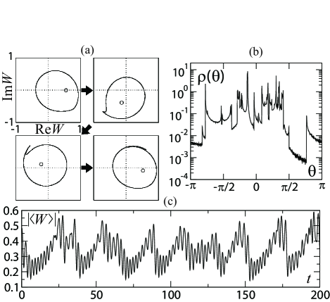
Figure 1: Collective chaos in globally-coupled limit-cycle oscillators [Eq. (1)] with $c_{1}=-2.0$, $c_{2}=3.0$, $K=0.47$, $N=10^{7}$. (a) Typical snapshots of the population in the complex plane; note the stretching and folding of the supporting line. (b) Typical distribution $\rho(\theta\equiv\arg W)$ for a configuration where no fold is present. (c) Time series $|\langle W\rangle|$.

To sum up the set of collective LE correspond to what one would expect from the observed global dynamics in Fig. 1c, and the action of the associated CLV also corroborates this view. Although strong finite-size effects couple macroscopic (delocalized) and microscopic (localized) modes, it is likely that, for the case studied above, no other collective mode exists, although we cannot exclude the emergence of other ones (in particular very weakly chaotic) at still larger sizes than those probed here. Thus, conventional Lyapunov analysis, supplemented with the calculation of covariant vectors, is able to capture the collective behavior of a large chaotic system. To investigate the generality of this finding, we now turn to systems of globally-coupled maps of one real variable.

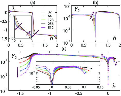
Figure 2: (color online) Spectra of $\lambda$ vs. $h$ (a), $Y_{2}$ vs. $h$ (b), and $Y_{2}$ vs. $\lambda$ (c) for the system depicted in Fig. 1 for different sizes $N$. Insets: close-ups of the positive branch. (Arrows indicate increasing $N$.)

In globally-coupled systems of identical units, one can look “directly” at the infinite-size limit by studying the evolution of the instantaneous distribution function of the values taken by the units, which is governed by the Perron-Frobenius operator. Although this is a difficult analytical task, a numerical approach, e.g., by using finer and finer binnings of the support of the evolving distribution, is in principle possible. In the case described above, this is made difficult by the fact that this support is the complex plane fractal-like curve described in Fig. 1a. For globally-coupled maps of a real variable, however, the support is typically a bounded interval of the real axis, so that a numerical integration is accessible. As a matter of fact, previous work on globally-coupled noisy logistic maps DeMonte_etal ; Shibata_etal-PRL1999 has provided partial evidence that the LE of the PF dynamics are related to the collective dynamics, but no direct link was ever shown. We thus consider the same system:

$$x_{i}^{t+1}=(1-K)f(x_{i}^{t})+K\langle f(x)\rangle+\xi_{i}^{t},$$ (2)

where $f(x)\equiv 1-ax^{2}$ is the logistic map (here we use $a=1.57$, in the one-band chaos regime) and $\xi_{i}^{t}$ is a delta-correlated noise. For an infinite system, the evolution of $\rho^{t}(x)$, the instantaneous distribution of $x$ values, is governed by the following nonlinear PF equation

$$\begin{array}[]{ll}&\rho^{t+1}(x)=\int\rho_{\rm N}(F^{t}(y)-x)\rho^{t}(y)\mathrm{d}y\\ {\rm with}&F^{t}(y)=(1-K)f(y)+K\int f(z)\rho^{t}(z)\mathrm{d}z\;,\end{array}$$ (3)

where $\rho_{\rm N}(\xi)$ is the noise distribution function. To evolve properly both Eq. (3) and its tangent space dynamics requires to keep the support of $\rho^{t}(x)$ within $[-1,1]$, the invariant interval of the logistic map, and to have well-defined derivatives of $\rho_{\rm N}(\xi)$, a fact overlooked by DeMonte_etal ; Shibata_etal-PRL1999 . We therefore use the bounded and differentiable noise Kumaraswamy distribution $\rho_{\rm N}(\xi)=15{\xi^{\prime}}^{2}(1-{\xi^{\prime}}^{3})^{4}$ with $\xi^{\prime}\equiv(\xi/\sigma+1)/2\in[0,1]$, so that $\xi\in[-\sigma,\sigma]$. We focus on the collective chaos regime observed for $K=0.28$ and a noise level $\sigma=0.1$, in which local dynamical variables tend to synchronize but are weakly scattered by microscopic chaos and noise Teramae_Kuramoto-PRE2001 ; DeMonte_etal .

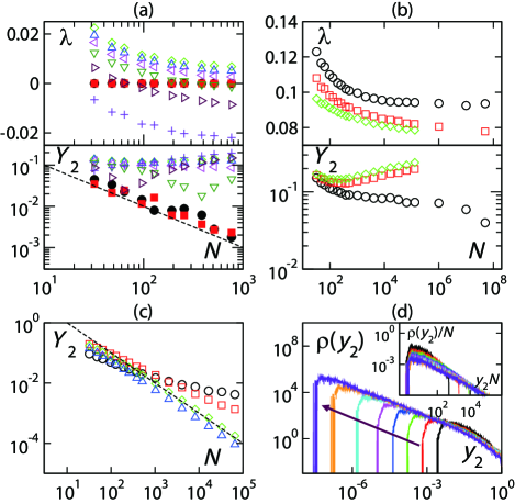
Figure 3: (color online) Size dependence for the system depicted in Figs. 1 and 2. (a) $\lambda$ and $Y_{2}$ vs $N$ around $\lambda=0$. The two modes with $\lambda=0$ are shown in filled symbols. (b) same as (a) for the first 3 modes. (c) $Y_{2}$ vs $N$ for the last four modes (d) Distribution of instantaneous $Y_{2}$ values for the first mode vs $N$. Inset: rescaling showing that eventually $Y_{2}\propto 1/N$. [The dashed lines in (a,c) correspond to the power-law $Y_{2}\sim 1/N$.]

We first describe the outcome of the conventional Lyapunov analysis. The $(\lambda,Y2)$ spectrum of small-size systems (Fig. 4a) reveals that the first few (positive) modes show signs of being delocalized. Calculating only the first three in large systems shows that the first mode is indeed delocalized, while the following ones are localized (Fig. 4c). Similar calculations do not indicate that any of the last modes is actually delocalized (data not shown). Thus, conventional Lyapunov analysis of finite systems seems to detect the presence of only one collective mode with exponent $\lambda_{N\to\infty}^{(1)}\simeq 0.081$ (Fig. 4b).

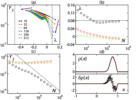
Figure 4: (color online) Lyapunov analysis for globally-coupled noisy logistic maps [Eq. (2)] with $a=1.57,K=0.28,\sigma=0.1$ and the corresponding PF equation [Eq. (3)]. (a) $(Y_{2},\lambda)$ spectra for different $N$. The vertical lines indicate the location of the first two LE of the PF dynamics. (b) First three LE vs system size $N$ (symbols) and for first PF LE (dashed line). (c) $Y_{2}$ vs $N$ for the first three modes [same symbols as in (b), the dashed line indicates the power law $Y_{2}\sim 1/N$]. (d) Typical snapshot for the distribution $\rho(x)$ (top) and for the first CLV $\delta\rho(x)$ (bottom). Solid lines and circles are the results from PF and maps of size $N=10^{7}$, respectively.

We now turn to our investigation of the PF dynamics. The evolution of $\rho(x)$ matches that of large collections of maps for a large number of timesteps (not infinite, due to finite-size and finite-binning effects), when taking for initial condition of the PF dynamics a (smoothed) instantaneous distribution of maps. The Lyapunov spectrum of the PF dynamics contains only one positive exponent $\lambda_{\rm PF}^{(1)}\simeq 0.0815$, in remarkable agreement with the “finite-size” collective exponent $\lambda_{N\to\infty}^{(1)}$ calculated above (Fig. 4b). Moreover, the CLV associated with $\lambda_{N\to\infty}^{(1)}$ and $\lambda_{\rm PF}^{(1)}$ share the same structure. In Fig. 4d, we show snapshots of each vector at timesteps carefully chosen so that the two distributions ($\rho(x)$ from the PF dynamics and the distribution reconstructed from a large-$N$ simulation) coincide very well (top panel). Both vectors exert the same shift in distribution $\delta\rho(x)$ (lower panel). Thus, the collective mode appearing in the conventional Lyapunov analysis is the first Lyapunov mode of the PF dynamics. However, the PF dynamics possesses infinitely-many modes, all negative except the first one in our case, and even the second one, given at $\lambda_{\rm PF}^{(2)}\simeq-0.49$, is not detected by conventional Lyapunov analysis, at least up to $N=131072$. In fact, PF modes with negative LE may not necessarily be present in the microscopic Lyapunov analysis. This is trivially true in the special case $K=0$ (no coupling), where all conventional Lyapunov modes are localized with the same, positive exponent, while PF dynamics shows infinitely many negative exponents which can be seen as superpositions of $O(N)$ independent microscopic modes. Whether this zero-coupling situation extends to coupled maps —and thus would explain how some PF negative modes could remain unseen in conventional spectra— is a difficult question which should be treated at a more mathematical level. We note finally that at least some negative collective modes appear in conventional Lyapunov analysis, as shown for Eq. (1), while positive PF modes are probably all present because they cannot be superpositions of independent microscopic modes. (Such perturbations would not grow.)

To summarize, we have shown, using generic globally-coupled systems, that conventional Lyapunov analysis can capture the collective dynamics of large chaotic systems through delocalization of CLV. We have found collective Lyapunov modes which are delocalized for large but finite system sizes, and clearly related to the observed macroscopic dynamics. This implies that there is no general need for finite-amplitude perturbations as claimed in some earlier studies Shibata_Kaneko-PRL1998 ; Cencini_etal-PhysD1999 . Moreover, we have directly identified, in one case at least, one such collective mode with a Lyapunov mode of the PF dynamics. Further results will be needed to strengthen these findings. We have studied other globally-coupled systems and reached similar conclusions Takeuchi_etal-TBP , but the strong “finite-size” coupling between microscopic and collective modes reported here makes it difficult to build a reliable asymptotic picture. We believe our conclusions should also hold for locally-coupled systems, which generically exhibit non-chaotic collective behavior, but first attempts in this direction have revealed even stronger size effects in this case.

At any rate, our results already imply that the conventional criterion usually adopted to prove the extensivity of (microscopic) chaos in large dynamical systems has to be changed. Collective modes should be excluded from the usual rescaling of Lyapunov spectra at least, but this may not be enough in practice, since microscopic modes are strongly influenced by neighboring collective modes through the finite-size effects reported above. Thus, an operative definition of chaos extensivity using Lyapunov analysis implies a quantitative understanding of these finite-size effects, a task left for future work.

We acknowledge fruitful discussions with A. Politi and M. Sano. This work is supported in part by JSPS.

References

- (1) D. Ruelle, Commun. Math. Phys. 87, 287 (1982).
- (2) See, e.g., P. Manneville, in Macroscopic Modelling of Turbulent Flows, Lecture Notes in Physics Vol. 230, edited by U. Frisch et al., (Springer-Verlag, Berlin, 1985), p. 319; R. Livi, A. Politi, and S. Ruffo, J. Phys. A: Math. Gen. 19, 2033 (1986).
- (3) H. Chaté and P. Manneville, Prog. Theor. Phys. 87, 1 (1992).
- (4) K. Kaneko, Phys. Rev. Lett. 65, 1391 (1990); A. S. Pikovsky and J. Kurths, Phys. Rev. Lett. 72, 1644 (1994).
- (5) T. Shibata and K. Kaneko, Phys. Rev. Lett. 81, 4116 (1998).
- (6) M. Cencini et al., Physica D 130, 58 (1999).
- (7) N. Nakagawa and Y. Kuramoto, Physica D 80, 307 (1995).
- (8) J. -P. Eckmann and D. Ruelle, Rev. Mod. Phys. 57, 617 (1985).
- (9) F. Ginelli et al., Phys. Rev. Lett. 99, 130601 (2007).
- (10) A. D. Mirlin, Phys. Rep. 326, 259 (2000).
- (11) M. Sano and Y. Sawada, Phys. Lett. A 97, 73 (1983).
- (12) One is quickly limited by numerical power when calculating the full spectrum of large systems, but the first few LE and CLV are accessible for larger sizes. For globally-coupled systems, this is also true of the last few modes.
- (13) K. A. Takeuchi et al., to be published.
- (14) T. Shibata, T. Chawanya, and K. Kaneko, Phys. Rev. Lett. 82, 4424 (1999).
- (15) S. De Monte et al., Phys. Rev. Lett. 92, 254101 (2004); Prog. Theor. Phys. Suppl. 161, 27 (2006).
- (16) J. Teramae and Y. Kuramoto, Phys. Rev. E 63, 036210 (2001).