Galaxy Zoo Green Peas: Discovery of A Class of Compact Extremely Star-Forming Galaxies

Abstract

We investigate a class of rapidly growing emission line galaxies, known as “Green Peas,” first noted by volunteers in the Galaxy Zoo project because of their peculiar bright green colour and small size, unresolved in SDSS imaging. Their appearance is due to very strong optical emission lines, namely [O III] $\lambda$5007 Å, with an unusually large equivalent width of up to $\sim$1000 Å. We discuss a well-defined sample of 251 colour-selected objects, most of which are strongly star forming, although there are some AGN interlopers including 8 newly discovered Narrow Line Seyfert 1 galaxies. The star-forming Peas are low mass galaxies (M$\sim 10^{8.5}-10^{10}$ ${\rm M_{\odot}}$) with high star formation rates ($\sim 10$ ${\rm M_{\odot}yr^{-1}}$), low metallicities (log[O/H] + 12 $\sim$8.7) and low reddening (${\rm E(B-V)\leq 0.25}$) and they reside in low density environments. They have some of the highest specific star formation rates (up to $\sim 10^{-8}$ ${\rm yr^{-1}}$) seen in the local Universe, yielding doubling times for their stellar mass of hundreds of Myrs. The few star-forming Peas with HST imaging appear to have several clumps of bright star-forming regions and low surface density features that may indicate recent or ongoing mergers. The Peas are similar in size, mass, luminosity and metallicity to Luminous Blue Compact Galaxies. They are also similar to high redshift UV-luminous galaxies, e.g., Lyman-break galaxies and Lyman-$\alpha$ emitters, and therefore provide a local laboratory with which to study the extreme star formation processes that occur in high-redshift galaxies. Studying starbursting galaxies as a function of redshift is essential to understanding the build up of stellar mass in the Universe.

1 Introduction

In this paper, we report on the discovery of an intriguing class of objects discovered by the Galaxy Zoo project. The Galaxy Zoo project (Lintott et al., 2008) has enlisted the help of over 200,000 members of the public to morphologically classify almost $10^{6}$ galaxies from the Sloan Digital Sky Survey (SDSS; York et al. 2000). The Galaxy Zoo website provides a randomly selected $gri$ composite colour image from the SDSS main galaxy sample and asks the volunteers to classify the morphology of the displayed object. One advantage of this distributed approach to classification is the fact that each object will receive multiple, independent classifications, and so one can treat the distribution of classifications for each object in a statistical sense. These classifications have led to numerous results in galaxy formation and cosmology (e.g., Skibba et al., 2008; Land et al., 2008; Bamford et al., 2009; Lintott, 2009; Schawinski et al., 2009; Slosar et al., 2009; Darg et al., 2009).

In addition to the website used for classification, Galaxy Zoo also provides an online discussion forum where volunteers may ask questions about unusual or challenging objects. This allows us to tap into another advantage of human classifiers: they can easily identify and then investigate odd objects. One such class of highly unusual objects was named ‘Green Peas’ as they appeared to be unresolved round point sources that looked green in the $gri$ composite. Figure 1 shows three example Pea images found by users, as well as a more typical galaxy at the same redshift (z$\sim$0.2). The volunteers rapidly assembled over a hundred of these objects in a dedicated discussion thread. Most of these were classified as stars in the SDSS photometric pipeline (Lupton et al., 2001). It quickly became apparent that these objects represent a distinct group: they all had galaxy-type spectral features (as opposed to broad-line quasar spectra or stellar spectra), and their green colour was driven by a very powerful [OIII] $\lambda$5007 Åemission line that substantially increased the $r$-band luminosity relative to the adjacent $g$ and $i$ band (green being the colour represented by the $r$-band in the SDSS colour composites). As a result of this selection, the Peas are found at redshifts $0.112\mathrel{\hbox{\hbox to0.0pt{\hbox{\lower 4.0pt\hbox{$\sim$}}\hss}\hbox{$<$}}}z\mathrel{\hbox{\hbox to0.0pt{\hbox{\lower 4.0pt\hbox{$\sim$}}\hss}\hbox{$<$}}}0.360$, mostly beyond the main galaxy sample but much nearer than luminous quasars. This discovery prompted our investigation into the nature of these small [O III]-emitters.

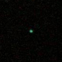
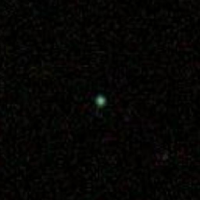
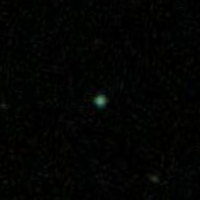
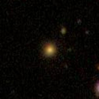
Figure 1: Example $g$,$r$,$i$ composite colour 50^′′x 50^′′  SDSS images classified by Pea hunters, with the $r$-band representing green light. The distinctly green colour and compact morphology makes the Peas (left 3 images) easily distinguishable from the classical elliptical (right image). The elliptical galaxy is clearly red and has a smooth profile, while the Peas are $r$-band dominated and unresolved in these images, appearing like stellar point sources. All objects shown here are at z$\sim$0.2.

In Section 2, we present the sample selection, and analyse their photometric properties (§ 2.1), space density (§ 2.2), morphologies in SDSS (§ 2.3), environments (§ 2.4), spectral properties (§2.5-§2.6) and HST imaging morphologies (§ 2.7). The Peas turn out to be largely star-forming objects with some AGN interlopers. We look into the nature of the few AGN Peas in Section 3. We study the nature of the star-forming galaxies in Section 4 and compare them to other known samples of galaxies in Section 5. Throughout this paper we assume $H_{0}=71\>{\rm km\>s^{-1}\>Mpc^{-1}}$, $\Omega_{\rm m}=0.3$ and $\Omega_{\rm\Lambda}=0.7$, consistent with the Wilkinson Microwave Anisotropy Probe 3-year results in combination with other cosmology probes (Spergel et al., 2007).

2 Data

2.1 Sample Selection

Our sample of Peas is taken from the SDSS DR7 spectroscopic sample (Abazajian et al., 2009). A survey of a quarter of the sky, the SDSS provides photometry of 357 million unique objects in five filters, $u$, $g$, $r$, $i$ and $z$ (Fukugita et al., 1996) and spectroscopy of many objects. Using the CasJobs application provided by SDSS, we uniformly searched the DR7 spectroscopic sample for Peas (originally noticed by eye in Galaxy Zoo) in the redshift range $0.112<z<0.360$ where the [O III] $\lambda$5007 Åline is in the $r$-band filter.

To define colour selection criteria, we compared the sample of $\sim$100 Peas identified by the Galaxy Zoo volunteers to a comparison sample of 10,000 galaxies and 9,500 QSOs at the same redshifts over the colour space defined by the 5 SDSS bands. The 10,000 galaxies were selected to match the redshift and $g$-band-magnitude distributions of the Peas. The QSO sample contains all spectroscopically confirmed QSOs in the Peas’ redshift range, because the QSOs are overall too luminous to match the Peas magnitude distribution. Figure 2 displays two colour-colour plots with Peas (green crosses), comparison galaxies (red points) and comparison QSOs (purple stars). The green Pea colour selection is shown by the darkened black lines. The precise colour cuts were selected to avoid both the QSO and overall galaxy sequences and to highlight the unusual objects selected by eye in the Galaxy Zoo forum. The colour limits are:

$$u-r\leq 2.5\\$$ (1)

$$r-i\leq-0.2\\$$ (2)

$$r-z\leq 0.5\\$$ (3)

$$g-r\geq r-i+0.5\\$$ (4)

$$u-r\geq 2.5(r-z)\\$$ (5)

We illustrate the effectiveness of this colour selection in Figure 2. It divides the Peas from the loci of both the galaxy and the quasar populations. This colour selection technique effectively uses the narrow-band survey technique common in high redshift galaxy searches, only here applying it to the broader SDSS filters. Because we are using broad filters, we are only sensitive to galaxies with extreme [O III] equivalent widths. Further, because we are using the $r$-band filter for colour selection, we are not sensitive to Pea-like objects at lower and higher redshifts. As seen in Figure 2, the Peas do indeed have distinct colours from the SDSS main galaxy sample. This is especially noticeable in the $r-i$ and $g-r$ colours used to create the 3-colour images. Using the colour selection, we find a sample of 251 Peas taken from all SDSS spectroscopic galaxies whose spectra we further analyse to understand their properties.

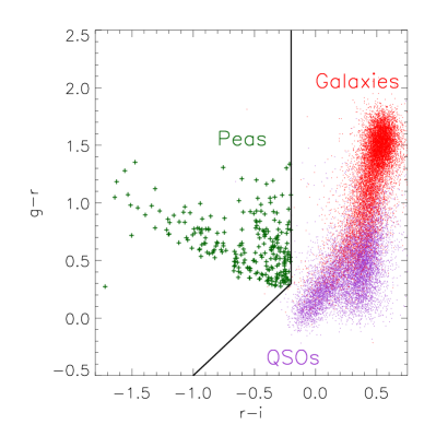
Figure 2: Left: $r-i$ vs $g-r$ colour-colour diagram for 251 Peas (green crosses) and a sample of normal galaxies (red points) matched in $z$ and $g$-band magnitude, and all QSOs (purple points) which lie in the same redshift range as the Peas, $0.112<z<0.36$. Right: $r-z$ vs $u-r$ colour for the same classes. The Peas are most cleanly separated in the $r-i$, $g-r$ colour diagram, where they stand out as particularly bright in the $r$-band. The colour cuts were selected to include the Peas identified by the Galaxy Zoo volunteers and to exclude both galaxies and QSOs.

Although most of the Peas were identified by the SDSS spectroscopic pipeline as having galaxy spectra (4 were classified as unknown), only 7 were targeted by the SDSS spectral fibre allocation as galaxies. Most were targeted as serendipitous objects, with the majority flagged as SERENDIP_BLUE, SERENDIP_DISTANT and TARGET_QSO_FAINT. These target flags are for objects lying outside the stellar locus in colour space and DISTANT here refers to distance from the stellar locus, QSO_FAINT is also used for objects flagged as stellar that are both fainter than $i$=20 mag and outside the stellar locus in colour space (Stoughton et al., 2002). These objects were targeted by fibers as they became available in a given field, so their selection function is not well determined. Without a uniform selection for the Peas across the sky, their absolute space density cannot be accurately assessed.

2.2 How common are the Peas?

Because the spectroscopic selection is biased in unquantifiable ways, i.e., based on the availability of a spectral fibre in a given pointing, the space density of the Peas is difficult to assess. In order to estimate the space density of the Peas in SDSS, we need to search the entire SDSS photometric catalogue for objects with our colour selection criteria. We note that the Pea colour selection can also return much higher redshift objects by finding other emission lines in the $r$-band filter. Therefore we first search the spectroscopic sample to help understand these contaminants. Dropping the Pea redshift selection limits, we find 198 objects at higher redshift in the spectoscopic sample which fall into our colour-selection region. These are mostly QSOs (only 4 have a spectral type labelled as galaxy by the SDSS pipeline), which cluster at redshifts z=1.2, where the 2800Å Mg II line falls into the $r$-band, and z=3.0, where the 1546 Å  CIV line falls into the $r$-band. Very roughly, in the entire spectroscopic database, there are comparable numbers of Peas and higher-z QSOs in the colour-selection region. Searching the entire SDSS photometric catalogue (PhotoObj) regardless of spectroscopic information, we limit ourselves to objects with the same $r$-band magnitude range as the Peas (18 $\leq r\leq$20.5) and to objects with similar compactness (petrorad_r $\leq$ 2.0 ^′′), in order to limit the contaminants from other redshifts. We further added the requirement of small $g$, $r$ and $i$ band photometric errors to avoid the scattering of contaminants with poor photometry into the colour selection region. This search returns 40,222 objects. The unique area of the SDSS DR7 footprint covers 8423 sq. deg, so this implies a rough spatial density estimate of 5 per square degree. Strictly speaking this is an upper limit because our selection likely still contains QSOs from higher redshifts. Looking at QSO number counts, we would expect to see $\sim$3 per sq. degree in our magnitude range (Richards et al., 2005), leaving two Peas per square degree brighter than 20.5 magnitudes. Therefore, we conclude the Peas are rare objects.

2.3 Morphology from SDSS imaging

Of the 251 Peas in our sample, 215 were classified as morphological type STAR and not as extended objects by the SDSS pipeline. Compared to the size of the galaxies as measured by the SDSS Pipeline (Petrosian radius: Blanton et al. 2001; Yasuda et al. 2001), they are significantly smaller. This is expected because the spectroscopic galaxy sample was selected to be both resolved and brighter than the faintest Pea (Strauss et al., 2002). The typical resolution of the SDSS images is large ($\mathrel{\hbox{\hbox to0.0pt{\hbox{\lower 4.0pt\hbox{$\sim$}}\hss}\hbox{$>$}}}1\hbox{${}^{\prime\prime}$}$), just below the peak of the sizes of the Peas as measured by the SDSS Petrosian radius. At the typical redshifts of the Peas, this angular scale corresponds to an upper limit on the physical half-light radius of approximately 5 kpc.

2.4 Environment

Because the Peas are at redshifts higher than the main spectroscopic galaxy sample, we measure the projected densities around the Peas and a sample of random galaxies matched in both luminosity and redshift, counting the number of projected neighbours within a radius of 1 Mpc and brighter than an absolute $i$-band magnitude of -20.5 at the redshift of the target are counted. This magnitude limit was selected to be well above the detection limit of the highest redshift Peas. Figure 3 shows the cumulative distribution of neighbour counts for the Peas (solid line) and the control sample of galaxies (dotted line). Although this is a simple test, neglecting foreground and background contamination in the neighbour counts, and hence underestimating the difference between high and low density environments, it is clear that the Peas inhabit significantly lower density regions than typical galaxies of the same $i$-band luminosity. A Kolmogorov-Smirnov test indicates that the difference is significant at a greater than 8-$\sigma$ level. We find the median environmental density around the Peas is less than two-thirds of that around normal galaxies.

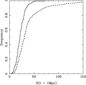
Figure 3: The cumulative distribution of neighbour counts for the Peas (solid line) is significantly different than a comparison galaxy sample (dotted line). No Peas live in the highest density environments.

2.5 Spectral Analysis

We downloaded all of the Peas’ spectra from the DR7 archive and carefully re-fit them, paying close attention to both the continuum and emission lines. We fit the stellar continuum and ionised-gas emission, following the technique of Sarzi et al. (2006), using the corresponding PPXF (Penalised Pixel Fitting; Cappellari & Emsellem 2004) and GANDALF (Gas AND Absorption Line Fitting) IDL (Interactive Data Language) codes adapted for dealing with SDSS data. Stellar population templates (Tremonti et al., 2004) and Gaussian emission-line templates were simultaneously fitted to the data. When it improved the overall fit (9 cases), the Gaussian emission line templates included both broad-line and narrow-line components for the Balmer Series.

To ensure acceptable fits, we limit our spectroscopic sample to those Peas with a S/N greater than 3 in the continuum near the H$\beta$ and H$\alpha$ regions (specifically, measuring the S/N in the bands 6350-6500Å  and 5100-5250Å). Additionally, we limited our emission-line classification sample to those Peas with a S/N $\geq 3$ detection in each of the emission lines: H$\alpha$, H$\beta$, [O III] $\lambda$5007 Åand [N II] $\lambda$6583 Å, following Kauffmann et al. (2003). We note that for many of our objects near z$\sim$0.3, sky lines fall on top of the [O III] line and the H$\beta$ line, and we removed all of these objects from our sample. One of these objects has broad Balmer lines, with both sky lines falling inside the H$\beta$ profile. This object is identified as a Narrow Line Seyfert 1 (NLS1) in the literature (Zhou et al., 2006), but we do not consider it further in this paper. These cuts result in a sample of 103 narrow-line objects to be further analysed (see § 2.6) plus nine objects best fit by a two-component Gaussian in the Balmer lines. The width of the broad Gaussian components ranged from just over 600 ${\rm km}$ ${\rm s}^{-1}$ to $\sim$5000 ${\rm km}$ ${\rm s}^{-1}$. Eight of these objects have FWHM narrower than 2000 ${\rm km}$ ${\rm s}^{-1}$ and are thus classified as Narrow Line Seyfert 1s (see §3). These eight SDSS spectroscopic objects have not previously been identified as NLS1s, (e.g., Williams et al., 2002; Zhou et al., 2006). Three examples of spectral fits are shown in Figure 4. The top 2 spectra are of narrow line objects and the bottom spectra shows a NLS1 object. In all three cases one can easily see a prominent [O III] doublet near $5007$ Å.

In summary, we have 9 Peas with two component fits, (1 broad Line Seyfert 1 and 8 Narrow Line Seyfert 1s) and 103 narrow line Peas.

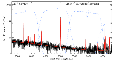
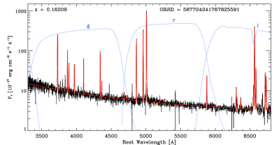
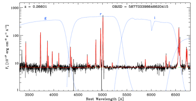
Figure 4: Example spectral fits from GANDALF. The top two plots show typical star-forming Peas and the bottom plot shows a typical Narrow Line Seyfert 1. In black is the rest-frame observed spectrum and in red the fit from GANDALF. The SDSS filter band passes are included as blue dotted line, shifted into the rest-frame of the Pea. Notice in all examples, the [O III] $\lambda$5007 Å  line is redshifted inside the $r$ bandpass. The Peas show very strong emission lines, including clear lines detected throughout the Balmer series.

2.6 Spectral Classification

The SDSS spectra cover the observed range 3800–9200 Å at a resolving power of R$\sim$1800. At the Peas’ redshifts, this range includes the regions around both the H$\beta$ and H$\alpha$ spectral lines. Example fits to these lines are shown in Figure 5.

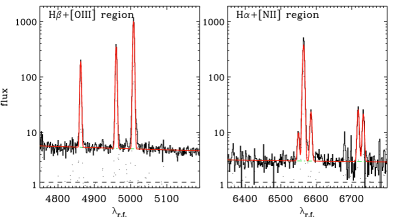
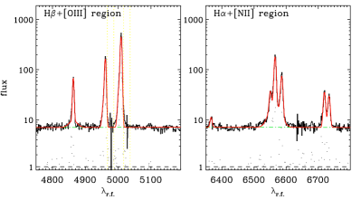
Figure 5: Example spectral fits from GANDALF in the regions around H$\alpha$ (right) and H$\beta$ (left). The top plots show a typical star-forming Pea and the bottom plots show a typical Narrow Line Seyfert 1.

We use a classical emission line diagnostic originally devised by Baldwin, Phillips & Terlevich 1981 (hereafter BPT) and modified by others (Osterbrock & Pogge, 1985; Veilleux & Osterbrock, 1987; Kewley et al., 2001, 2006; Kauffmann et al., 2003) to classify the narrow line objects. Emission line diagnostics probe the nature of the dominant ionising source and separate the galaxies dominated by ongoing star formation from those dominated by non-stellar processes (namely Seyfert and LINER galaxies). The classical BPT diagram, which compares the ratio of [O III] $\lambda$5007 Å/H$\beta$ to [N II] $\lambda$ 6583 Å/H$\alpha$, has been shown to be an efficient measure of the ionising source in a galaxy (Kewley et al., 2006). Additionally, Kewley et al. (2001) calculated the maximum starburst contribution from theoretical models, including modern stellar population synthesis, photoionisation and shock models (labelled Ke01 in Figure 6). Kauffmann et al. (2003) empirically shifted this line to separate purely star-forming objects from the rest using a set of $\sim 23,000$ SDSS spectra (labelled Ka03 in Figure 6). Objects that lie in between the Ke01 and Ka03 lines are transition galaxies containing a mix of star formation and a central AGN component (Kewley 2006). We note that the SDSS spectral fiber includes only the light of the central 3^′′ of the galaxy, so emission originating from the central AGN-ionised regions can be mixed with emission originating from extended star formation.

Table 1: Spectroscopic Classification

Type	Number
Broad Line AGN (Seyfert Type 1)	1
Narrow Line Seyfert 1s	8
Narrow Line AGN (Seyfert Type 2)	10
Transition Objects	13
Star Forming	80
Total	112

Analysis of the narrow-line Peas’ spectra (Figure 6) revealed that the majority of the objects are star forming (80, red stars), but there are also 10 Seyfert 2 (blue diamonds) and 13 transition objects (green crosses). The location of the star-forming galaxies in the top left of the BPT diagram indicates they likely have lower metallicity. This sample of galaxies is discussed in greater detail in § 4. In Table 1, we summarise the spectroscopic identifications.

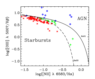
Figure 6: The BPT diagram classifies 103 narrow-line Peas (all with S/N $\geq$3 in the emission lines) as 10 AGN (blue diamonds), 13 transition objects (green crosses) and 80 starbursts (red stars). Solid line: Kewley et al. (2001) maximal starburst contribution (labelled Ke01); Dashed line: Kauffmann et al. (2003) line separating purely star-forming objects from AGN (labelled Ka03). The clustering of the starbursts in the top left corner of the plot indicates that they likely have low metallicity.

2.7 Morphology from HST imaging

Because the SDSS resolution is too low to measure the actual sizes of the Peas, we searched the HST archive, MAST, finding 5 public images. The observations are summarized in Table 2.

We reduced the ACS data, starting with the pipeline-reduced *flt* images and using multidrizzle to remove cosmic rays and defects, correct for distortion, and improve sampling of the PSF with a final scale of $0.04\hbox{${}^{\prime\prime}$}/{\rm pixel}$. In the case of the WFPC2 data, we started with the pipeline-reduced *c0f* images and used drizzle with parameters pix.scale=0.5 and pix.frac=0.8, leading to a final scale of 0.023 ^′′/pixel for the PC chip and 0.05 ^′′/pixel for the WF4 chip, respectively. Figure 7 shows all 5 public HST images of the Peas compared to a single typical ground-based SDSS image (bottom right).

For the ground-based image (Fig 7; bottom right), the SDSS archive lists a Petrosian radius of 1$.\!\!^{\prime\prime}$8, roughly 8 kpc at the Pea’s redshift (z=0.2832). This object is clearly unresolved when compared to the HST image of the same galaxy (top right) and the size as measured by the SDSS pipeline is therefore an upper limit. Of the 5 Peas with HST data, one is classified as a NLS1 (see §3; bottom centre image), three are identified as star forming (see §4; top images) and the last one has sky lines over the [O III] region and is thus unclassified (see §2.5; bottom left). The three star-forming galaxies were imaged as part of a study of local UV-luminous galaxies (Heckman et al., 2005; Overzier et al., 2008). All three Peas classified as starburst galaxies reveal complex structures too small to be resolved in ground-based imaging. The morphology of the top right object for example, shows several “knots” instead of one central component. These knots may be different star-forming regions, suggesting a morphology typical of merger events. Although the Peas live in low density environments, their star formation could still be driven by merging activity. The top centre image shows a central component with extended structures that look like two tidal tails reaching out to the east and south, possibly connecting to another galaxy in the south. The centre of the top left image seems also to consist of at least two knots rather than a smooth overall light distribution. The NLS1 (bottom centre) is from a study of AGN host galaxies (Schmitt, 2006) and the last object (bottom left) was imaged serendipitously in a study of Kuiper belt objects (Noll, 2007). In contrast to the star-forming galaxies, the NLS1, bottom centre, looks like a spiral seen edge on. This AGN aside, all of the HST images reveal complex structures much too small to be resolved in ground based imaging. Although our statistics are too low to make any conclusions on the general nature of the Peas, this is an interesting trend.

Table 2: HST Images

SDSS Obj ID	RA (J2000)	Dec(J2000)	z	Instrument	Chip	Filter	Exposure Time (s)	Figure location
587731187273892048	351.41345	0.75201	0.2770	WFPC2	PC	F606W	3600	top left
588013384341913605	141.50168	44.46004	0.1807	ACS	WF	F850LP	2274	top centre
587724199349387411	10.22636	15.56935	0.2832	WFPC2	PC	F606W	3600	top right
587726879424118904	344.49532	-8.62438	0.3081	ACS	WF	clear	1071	bottom left
587726032799400204	211.91701	2.29671	0.3092	WFPC2	WF4	F814W	1200	bottom centre

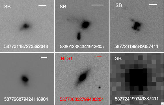
Figure 7: Hubble Space Telescope images of all Peas available in the archive. In each panel, we indicate a physical scale of 3 kpc at the redshift of the object (bar in top right of image). In the top row, we show three Peas classified as actively star-forming by their emission line ratios. In the bottom row, from left to right, an unclassified Pea, a Pea classified as a NLS1 and an SDSS image of a star-forming Pea at the same scale to highlight the degree to which the Peas are unresolved in typical SDSS imaging. These HST images illustrate that the upper limit on the Peas’ physical scale based on ground-based SDSS imaging is a significant overestimate of the true physical size. Furthermore, these HST images reveal that the star-forming Peas exhibit a complex morphology indicative of significant disturbances that may be due to mergers and/or clumpy regions of star formation or extinction.

3 The Properties of Narrow Line Seyfert 1 Peas

NLS1s constitute $\sim$15% of low redshift (z$\leq$0.5) Seyferts (Williams et al., 2002) and are characterised by H$\beta$ line widths broader than classical narrow-line AGN but narrower than classical Seyfert 1 galaxies. They appear to have Eddington ratios near 1 and black hole masses below the typical M_BH-$\sigma$ relation, suggesting a time delay between the growth of the galaxy and the growth of the central black hole mass (Ryan et al., 2007). Several authors use the [OIII] line as a surrogate for the bulge stellar velocity dispersion $\sigma$, assuming that the velocity field of the narrow-line region is dominated by the stellar gravitational potential (e.g., Bonning et al. 2005). However, the [OIII] line is known to often exhibit a blue wing that is associated with gas outflow and this can affect mass determinations (Marconi et al., 2008). Thus, Komossa et al. (2008) fit the blue wing separately and use only the main [OIII] component to estimate $\sigma$. This careful fitting can decrease the galaxy host mass measurement, placing the Narrow Line Seyfert 1 on the M_BH-$\sigma$ relation (Komossa et al., 2008).

Eight of the Peas are classified as NLS1s, which we define as galaxies with $500\leq{\rm FWHM}_{\rm{H}\beta}\leq 2000~{}{\rm km}~{}{\rm s}^{-1}$. We determined the black hole and galaxy masses for our sample of NLS1s. Black hole masses are estimated using the relation given by McLure & Jarvis (2002):

$${\rm M}_{\rm BH}=10^{7.63}{\rm v}_{3000}^{2}{\rm L}_{44}^{0.61}~{}M_{\odot},$$ (6)

where v₃₀₀₀ is the FWHM of the H$\beta$ line divided by 3000 km/s and $L_{44}$ is the luminosity at 5100Å divided by $10^{44}~{}\rm erg~{}s^{-1}$. To determine the galaxy mass, we fit the [O III] emission line with both a central narrow component and an additional blue wing. We then take the central narrow component as a proxy for the stellar velocity dispersion $\sigma$.

Figure 8 shows the stellar velocity dispersion of the bulge, estimated from $\sigma_{\rm[OIII]}$, vs black hole mass for the NLS1s, nearly all of which lie well below the classical M-$\sigma$ relation (solid line, Tremaine et al. (2002); dashed lines are 1-$\sigma$ error contours) even though we fit the [O III] line with an additional blue wing component. This contrasts with a recent study that found this fitting method puts the NLS1s nearer to the M-$\sigma$ relation (Komossa et al., 2008). Instead, our results are consistent with studies measuring the galaxy mass using near-infrared bulge measurements (Ryan et al., 2007). We also note that single broad-line AGN found in our sample is consistent with the M-$\sigma$ relation. Therefore the properties of our sample of NLS1s are consistent with some of those found in the literature, and can help in the study of the location of NLS1s on the M-$\sigma$ relation.

To better characterise the nuclear emission using high energy data, we searched the database at HEASARC for additional data on our sample. Unfortunately, the Peas are well distributed throughout the 8,400 square degrees covered by the SDSS and not concentrated in any of the areas covered by deep multi-wavelength surveys. None of the NLS1s are bright enough at soft X-ray wavelengths to be detected in the ROSAT All-Sky Survey (Voges et al., 1999). We note that the broad-line AGN is detected with a luminosity of nearly $10^{44}\rm{ergs}$ $\rm{s^{-1}}$, as is one of the type 2 Seyferts with an X-ray luminosity of nearly $3\times 10^{44}\rm{ergs}$ $\rm{s^{-1}}$ (0.2-2 keV). Given the redshift range of the Peas and the detection limits of the Rosat all sky survey, this limits the NLS1s’ X-ray luminosity to below a few $\times 10^{44}\rm{ergs}$ $\rm{s^{-1}}$; however, this upper limit is still well within the typical range of Seyfert luminosities.

One of the HST images is of a NLS1 Pea (Figure 7, bottom centre). This galaxy looks distinctly different from the patchy HST images of the Peas powered by star formation. It appears to be an edge on disk, with no sign of morphological disturbance. This is consistent with what is seen in the morphologies of other samples of NLS1s (Ryan et al., 2007).

Figure 8: Using the [OIII] width as a measure of the host galaxy mass, we plot one broad-line AGN (star) and eight NLS1s (diamonds) on the ${\rm M_{BH}}$-$\sigma$ relation. The NLS1s mostly lie far below the standard ${\rm M_{BH}}$-$\sigma$ relation, even though we determined galaxy mass from the narrow [OIII] component only.

Table 3: Narrow Line Seyfert 1s

SDSS ObjId	RA [degs]	Dec [degs]	z	$\sigma_{\rm[OIII]}$ [${\rm km~{}s^{-1}}$]a	MBH[$10^{7}M_{\odot}$]b
587726032799400204	211.917006	2.296711	0.30920	240.45 (4.47)	0.100 (0.024)
587733410983182549	214.828750	51.044473	0.32363	297.90 (8.69)	0.429 (0.239)
587733398646620415	245.539241	35.352080	0.26601	129.72 (2.47)	1.270 (0.323)
587731521734640128	117.387347	28.568545	0.33697	226.91 (4.96)	1.883 (0.599)
587731892187037787	172.279625	57.934812	0.31238	305.33 (3.50)	0.287 (0.103)
588017978351616137	171.563561	38.971510	0.33651	246.36 (4.38)	0.102 (0.026)
587739377230610665	124.500818	19.302802	0.32452	320.52 (3.83)	1.081 (0.329)
587739406266728813	239.238254	21.520959	0.23314	356.63 (3.31)	0.720 (0.139)

^a We measured the [OIII] line width fitting simultaneously for a blue wing and narrow Gaussian components. The measurements reported here are for the narrow Gaussian component with 3 sigma measurement error in parentheses.
^b The black hole masses are determined as in Eqn 1, 1 sigma errors are in parentheses.

4 The Properties of Star-Forming Peas

From our spectral diagnostics we have 80 star-forming objects, with high signal-to-noise, which we look at in greater detail here. They are listed in Table 4, where we include information from the SDSS DR7 archive in Columns 1-5: SDSS ObjId, RA, Dec, z and the equivalent width of [O III].

4.1 Star Formation Rates

To determine accurate star-formation rates using the H$\alpha$ fluxes, we corrected these recombination fluxes for both interestellar extinction and for the underlying stellar absorption lines in the stellar continuum (Kennicutt, 1998). We measured the Balmer decrement, assuming an ${\rm R_{V}=A_{V}/E(B-V)}=3.1$, and using the Cardelli et al. (1989) reddening curve and an intrinsic H$\alpha$ / H$\beta$ value of 2.85 (the Balmer decrement for case B recombination at T=$10^{4}$ K and $n_{e}=10^{4}$ cm^-3; Lequeux 2005). There are a handful of star-forming Peas with H$\alpha$ / H$\beta$ less than 2.85, but these measurements are due to a combination of intrinsically low reddening and uncertainty in line flux determinations (Figure 9, top panel); we set the extinction equal to zero in these cases. Overall, we find that the reddening values for the Peas are low (Figure 9, bottom panel), with nearly all Peas having ${\rm E(B-V)\leq 0.25}$. Finally, using the corrected H$\alpha$ flux measurements, we measured star-formation rates (Kennicutt, 1998) up to $\sim 30$ ${\rm M_{\odot}yr^{-1}}$. The measured star formation rates are added to table 4 in Column 7.

Figure 9: The histograms of H$\alpha$ / H$\beta$ (top) and the colour excess, $\rm E(B-V)$, (bottom) as determined from the Balmer decrement. This distribution indicates that the line-emitting regions of star-forming Peas are not highly reddened, particularly compared to more typical star-forming or starburst galaxies.

4.2 Stellar Mass

The optical spectral energy distribution (SED) of the Peas is dominated by their strong nebular emission lines. Thus we cannot apply standard SED fitting techniques directly to their photometric data. Additionally, virial masses are inaccessible due to the low S/N of the spectral continuum and our inability to fit absorption lines. We therefore turn to the SDSS spectra, where the emission lines can be subtracted or blocked out where necessary. The continuum of the resulting emission-line-free spectrum has very poor signal-to-noise, so rather than fit this spectrum directly, we convolve it with a set of 19 medium-band filters (Taniguchi, 2004) and treat the result as medium-band photometric data. In other words, we construct an SED from the spectral continuum. To this, we add the GALEX near- and far-UV photometric data points where available (§ 4.5) and fit the SED with stellar population models.

We employ a method similar to that of Schawinski et al. (2007) and model the star formation history with two bursts, to account for the possible presence of an underlying old stellar population. We use the stellar models of Maraston (1998, 2005) with the Salpeter IMF and a range of metallicities. We also account for dust extinction following the Calzetti et al. (2000) law and fit the resulting model photometry to the data and compute the $\chi^{2}$ statistic. After marginalising over all parameters, we obtain a stellar mass and an estimate of its error. Higher S/N spectra are required to constrain the mass ratio between with older and younger stellar components. Therefore our systematic errors are much larger than the computed formal statistical errors. To quantify this uncertainty, we compared our mass estimates using a second SED-fitting code (Kriek et al., 2009), again using a Salpeter IMF and Maraston (1998, 2005) models. The second code fits a single model template and therefore measures only a young stellar population component, excluding the additional free parameter of a second older stellar population from Schawinski et al. (2007). The single stellar population fits result in a total stellar mass 0.75 dex lower on average. This result is not unexpected as a younger stellar population is more luminous and can account for the same amount of light with a smaller mass contribution. Accounting for the average 0.75 offset between the two mass measurements, the residual dispersion was just under 0.3 dex. Therefore each individual mass measurement is uncertain at this minimum level. Because two stellar populations are more likely to reside in these galaxies (§ 5.1), we quote the masses from the two-burst model for the results in this paper acknowledging their uncertainty. Figure 10 shows an example stellar population fit. The median stellar mass of a Pea in our sample $\sim 10^{9.5}M_{\odot}$ and they range from $10^{8.5}M_{\odot}$ to nearly $10^{10.5}M_{\odot}$, indicating the Peas as a class are significantly less massive than an L_⋆ galaxy. Galaxy mass estimates are also included in Table 4, Column 9.

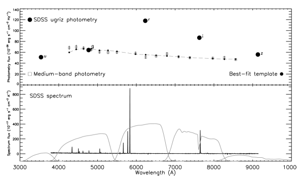
Figure 10: An example SED fit to a typical starforming Pea. The top panel shows both the original emission-line dominated SDSS $ugriz$ photometry (large black points), and the medium-band photometry derived from the emission-line subtracted spectrum used for the SED fit (open boxes). The best-fit template (small black points and dashed line) is plotted on top. In the bottom panel, we show the SDSS spectrum of this Pea together with the $ugriz$ filter transmission curves. The [OIII] line dominates the $r$-band flux and the $i$-band flux is significantly affected by H$\alpha$ emission. The SDSS broad-band photometry is dominated by emission lines to such an extent that fitting stellar templates to it cannot yield reliable results.

4.3 Metallicity

We measure gas phase metallicity for the Peas using [N II] $\lambda$6584 Å/ [O II] $\lambda\lambda$3726, 3729 Åto estimate log[O/H] + 12 (Kewley & Dopita, 2002). The average Peas has a metallicity of log[O/H] + 12 $\sim 8.7$. These metallicity measurements are broadly consistent with those determined from other line ratios for which we have lower (S/N) and fewer galaxies with measurements as well as with the location of the Peas on the BPT plot (Figure 6). We plot the Peas on the mass metallicity relation from Tremonti et al. (2004) in Figure 11. The lines are from Tremonti et al. (2004), enclosing 68% (dotted) and 95% (dashed) of the star-forming galaxies in the Tremonti et al. (2004) sample. Although we do not see a trend in the Peas’ metallicity with mass, they are roughly consistent with the mass-metallicity relation. The exception to this agreement is for the Peas with the largest masses, which have the same low metallicity as their lower-mass counterparts and therefore lie below the mass-metallicity relation. This is likely due to the uncertainty in the mass determinations rather than the measurement of gas phase metallicity. We include metallicity in Table 4, Column 8.

Overall, we find the Peas have log[O/H] + 12 $\sim 8.7$, sub-solar (Z${}_{\odot}\sim$0.5) as per measurements of Grevesse & Sauval (1998) and helioseismic measurements (Basu & Antia, 2008), but near the solar abundances of Asplund et al. (2005). These metallicities are common in low mass galaxies like the Peas.

Figure 11: The mass metallicity relation after Tremonti et al. (2004). The Peas are sub-solar metallicity. Although the Peas are in general consistent with the mass-metallicity relation, they depart from it at the highest mass end and thus do not follow the trend. The Peas selection selects galaxies with a range of masses, but a more uniform metallicity.

4.4 Specific Star Formation Rate

Combining the mass measurements with the star formation rates, we find extraordinarily high specific star formation rates for the Peas. “Specific” star formation rate (SSFR) refers to the star formation rate per solar mass in units of year^-1 and thus can be directly related to the time taken to double the stellar mass of a system (1/SSFR). In Figure 12 we compare the Peas to the Galaxy Zoo Merger Sample (Darg et al., 2009). Major mergers are frequently sites of active star formation, and yet the Peas are an order of magnitude higher in specific star formation rates than this comparison sample. These specific star formation rates imply doubling times between 100 Myr and $\sim 1$ Gyr. The uniformly high star forming rates of the Peas are not unexpected because their selection criteria targets strong emission lines. If the rates of star formation were lower, they would not be detected as “green” in the SDSS imaging. However, the SSFR we measure are unusually high for galaxies at z$\sim$0.2, which typically reach SSFR$\sim 10^{-9}$yr^-1 at most (Brinchmann et al., 2004; Bauer et al., 2005).

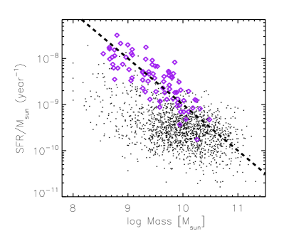
Figure 12: Specific star-formation rate vs. mass for the Peas (purple diamonds) and the Galaxy Zoo Mergers sample (black points). The Peas have low masses typical of dwarf galaxies and much higher specific star formation rates compared to the merging galaxies. The dashed line shows a constant star formation rate of 10 M_⊙yr^-1. Most of the Peas had SFRs between 3 and 30 M_⊙yr^-1 and hence follow this line closely.

4.5 UV Luminosity

The Peas are well spread throughout the 8,400 square degrees covered by the SDSS and not concentrated in any of the areas covered by deep multi-wavelength surveys. However, GALEX GR4 is well matched to SDSS in depth and area and 139 of the 251 Peas are detected in GALEX GR4 data (Morrissey et al., 2007). For the 57 of 80 star-forming Peas with Galex detections (S/N $\geq$ 3), the median luminosity is $3\times 10^{10}L_{\odot}$. We include L_FUV in Table 4, Column 6. The very high UV luminosities combined with low reddening (§4.1) are rare in local galaxies and are more typically found in galaxies at higher redshift.

5 Comparison with other samples of galaxies

5.1 Blue Compact Dwarfs

Blue compact dwarfs are a subset of the local dwarf population, first identified by Zwicky (1965) as star-like field galaxies on Palomar Sky Survey Plates. They are characterized by compact, gas-rich regions of high star formation rates (Papaderos et al., 2002; Vaduvescu et al., 2007), often lying inside an older stellar population of larger spatial extent containing a significant mass contribution of the galaxy as a whole (Loose & Thuan, 1986; Kunth et al., 1988; Papaderos et al., 1996; Aloisi et al., 2007). They are generally low-metallicity (7.12 $\leq$ 12+log(O/H) $\leq$ 8.4), evolved, gas-rich dwarfs undergoing recurrent starburst activity (Loose & Thuan, 1986; Papaderos et al., 1996; Gil de Paz & Madore, 2005; Papaderos et al., 2008). As a class Blue Compact Dwarfs cover a wide range in absolute magnitude and are often sub-classified by size (Ultra Compact Blue Dwarfs) or luminosity (Luminous Blue Compact Galaxies).

Ultra Compact Blue Dwarf galaxies are the smallest of the Blue Compact Dwarfs with physical diameters less than 1 kpc and low masses ($\sim$ $10^{7}-10^{9}$M_⊙; Corbin et al. 2006). Typically an order of magnitude less luminous than other BCGs, their optical spectra can be dominated by very strong emission lines (Guseva et al., 2004; Corbin et al., 2006) and they can contain substantial amounts of internal dust (eg. $E(B-V)\sim 0.28$ ; Corbin & Vacca 2002). Like other low mass galaxies, Ultra Blue Compact Dwarfs have very low metallicities, yet they still lie on an extrapolation of the Tremonti et al. (2004) mass-metallicity relation (Corbin et al., 2006). These galaxies can show asymmetric morphologies with multiple sub-clumps of active star-forming regions (Corbin & Vacca, 2002; Corbin et al., 2006). While their light is dominated by the compact, young ($\sim$1-10 Myr) stellar population, their stellar mass is dominated by an older, evolved ($\sim$10 Gyr) population. As a population, these galaxies tend to reside within voids (Corbin et al., 2006).

At the other end of the Blue Compact Dwarf category, Luminous Blue Compact Galaxies are the most luminous members with $M_{B}\leq-17.5$. They are more massive than their Ultra Compact counterparts, with average masses near 5$\times$10⁹ M_⊙ (Guzmán et al., 2003). As one might expect from a class of more massive galaxies, their metallicities are on average higher than the Ultra Blue Compact Dwarfs (7.7 $\leq$ 12+log(O/H) $\leq$ 8.4; Guseva et al. 2004; Hoyos et al. 2007). However, like their Ultra Compact Blue Dwarf counterparts, Luminous Blue Compact Galaxies show compact prominent regions of star formation, often with disturbed morphologies (Bergvall & Johansson, 1985) and star formation rates typically ranging from 1-5 M${\rm{}_{\odot}yr^{-1}}$. Underlying these young, star-forming regions, older stellar populations with the colours and stellar profiles of older, massive ellipticals are detected in near-IR imaging (Bergvall & Östlin, 2002). Examples of Luminous Blue Compact Galaxies are found at intermediate redshifts (Guzman et al., 1997; Phillips et al., 1997; Hoyos et al., 2004) and may contribute up to 50% of the star formation rate density in the Universe at z=1 (Guzman et al., 1997).

Because both the Peas and Blue Compact Dwarf galaxies contain strong emission lines originating in compact regions of star formation, we investigated their potential overlap as a class. Although the Peas are similar in morphology, environment and physical size to the z=0 Ultra Blue Compact Dwarfs, they appear to be a different class of galaxies. The Peas have significantly higher metallicities, typically more than 0.5 Z_⊙ compared to 0.02 Z_⊙ for the Ultra Compact Blue Dwarfs. Additionally, the stellar masses of the Peas are on average $\sim$10^9.5M_⊙, roughly an order of magnitude larger than similar measurements of Ultra Compact Blue Dwarfs (Corbin et al., 2006). While Ultra Compact Blue Dwarfs are found near $z\sim 0$, the Peas are detected at 0.113$\leq$z$\leq$0.36, meaning they have several Gyrs to grow and further increase their metallicity before reaching z=0, increasing the disparity in the measured masses and metallicities. In contrast, the largest of the Blue Compact Dwarfs, Luminous Blue Compact Galaxies have stellar masses and metallicities that match the measured values for the Peas. The luminosities of the Peas are easily as bright as this class of galaxies, with median $M_{B}\sim-20$. Additionally, studies of low-metallicity SDSS objects like Blue Compact Dwarfs find that they lie in the same location on the BPT plot shown in Figure 6 (Izotov et al., 2006) and [O III] 5007 / H$\beta$ line ratios for a sample of four Luminous Compact Blue Galaxies measured with STIS ($\log([OIII]\lambda 5007\AA~{}H\beta)\sim 0.5$; Hoyos et al. 2004) are similar to those we find here (Figure 6). Studies of the Peas at near-infrared wavelengths could potentially reveal older stellar populations, like those found in Luminous Blue Compact Galaxies. These older stellar populations could reveal additional stellar mass and potentially larger radii. Therefore, the Peas could potentially be classified as part of the heterogeneous Luminous Blue Compact Galaxies category.

We tentatively conclude that the Peas form a different class of galaxies than Ultra Blue Compact Dwarfs, but they are similar to the most luminous members of the Blue Compact Dwarfs category, Luminous Blue Compact Galaxies.

5.2 Local UV-Luminous Galaxies

Heckman et al. (2005) defined a sample of 215 ultraviolet-luminous galaxies (UVLGs) from the SDSS spectroscopic galaxy sample (DR3) and GALEX (GR1) with luminosities $L_{\rm FUV}\geq 2\times 10^{10}L_{\odot}$. We have 139 Peas with Galex detections (S/N $\geq$ 3), 44 of which meet Heckman et al. (2005)’s criteria ($L_{FUV}\geq 2\times 10^{10}L_{\odot}$, z$\leq$0.3 and SDSS pipeline spectral type identified as galaxy. Since GR4+DR7 cover a much larger area than GR1+DR3, we find only four overlapping sources between the Peas and the UVLG sample (Hoopes et al., 2007). However, we note that none of the other 211 UVLGs fall into the SDSS colour-selection wedge of the Peas.

The Peas selection includes many UV-luminous galaxies, but does not uncover the same population of galaxies as a selection based on UV luminosity. To illustrate this in Figure 13, we compare the [O III] equivalent width, as measured by the SDSS pipeline, for the galaxy sample described in Section 2.1 and the Heckman et al. (2005) UVLG sample to that of the Peas. Unsurprisingly, due to their selection, the Peas have much larger equivalent width measurements than either the UVLG sample or the general spectroscopic galaxy sample (§ 13). The Pea [O III] equivalent widths are due to the combination of both very high star formation rates and the faint continuum. The Peas form a sample of objects selected to have large [O III] equivalent widths, many of which also have large UV luminosities. As the UVLGs are currently one of the best local samples of galaxies analogous to high redshift Lyman-break galaxies (Hoopes et al., 2007), we now look into the comparison between the Peas and high redshift galaxy samples.

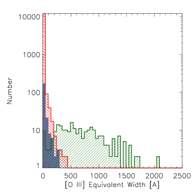
Figure 13: Neither the distribution of [O III] equivalent width for $\sim 10,0000$ comparison galaxies (§2.1; red lined histogram) nor the UVLG sample (blue solid histogram) have equivalent widths comparable to the Peas (green lined histogram). As a class the Peas have much larger [O III] equivalent widths than normal or UV-luminous galaxies. All equivalent widths displayed here are from the SDSS pipeline measurements.

5.3 UV-luminous High Redshift Galaxies

Peas are sites of extreme star-formation in the local Universe. They are both very compact and have low stellar masses, yet they have enormous star formation rates, as shown by their emission lines and their UV luminosity. This sample of galaxies is quite distinct from typical $z\sim 0$ star-forming galaxies, i.e., blue spiral galaxies or dusty irregulars (Kennicutt, 1998). Therefore, we look at the properties of higher redshift galaxies where the bulk of the star formation in the Universe is occurring (Madau et al., 1996; Lilly et al., 1996; Reddy & Steidel, 2009).

Various colour-selection techniques have been developed for selecting samples of high redshift galaxies, including the Lyman-break dropout technique, which selects $z\sim 3$ galaxies by identifying $U$-band dropouts in deep imaging (e.g., Steidel et al. 2003), and Ly$\alpha$ emission selection, which uses narrow-band imaging to select galaxies at various redshifts due to the excess emission of Ly$\alpha$ compared to the neighbouring continuum (Cowie & Hu, 1998; Thommes et al., 1998; Kudritzki et al., 2000; Steidel et al., 2000). Both techniques return a similar population of galaxies, but Ly$\alpha$ emitters are characterised by a fainter continuum and stronger equivalent widths in their emission lines (Giavalisco, 2002). Although both selection techniques have different biases, the galaxies showing Ly$\alpha$ in emission tend to be smaller and younger on average (Gawiser et al., 2007; Finkelstein et al., 2007). UV-luminous high redshift galaxies, like Ly-$\alpha$ emitters and Lyman-break galaxies, are characterized by a high UV luminosity and a relatively low obscuration by dust (Gawiser et al., 2006; Venemans et al., 2005). They are starburst galaxies with strong blue continua dominated by young, massive stars (Giavalisco, 2002). These techniques have been extended to other redshifts out to $z\sim 6$, using different photometric bands to select drop-out galaxies (e.g., Ouchi et al. 2001; Stanway et al. 2003; Giavalisco et al. 2004; Kakazu et al. 2007). In a broad sense, the Peas are an application of a Ly$\alpha$-like selection technique at much lower redshift and targeting the [O III] emission line.

UV-luminous, high-redshift galaxies are similar in size to the Peas, with half light radii $\mathrel{\hbox{\hbox to0.0pt{\hbox{\lower 4.0pt\hbox{$\sim$}}\hss}\hbox{$<$}}}$ 2 kpc (Giavalisco et al., 1996; Bremer et al., 2004; Pascarelle et al., 1998). Many of these high redshift galaxies show disturbed morphologies (Ravindranath et al., 2006; Lotz et al., 2006), like those seen in the HST images of the star-forming Peas in Figure 7. In Lyman-break galaxies, rest-frame equivalent widths of [O III] can reach up to hundreds of Å  (Pettini et al., 2001), although most are much lower. For Ly$\alpha$ emitters, most are selected to have EW of Ly$\alpha$ $\geq$ 20 Å and can range up to $\sim$240 Å  or more (Gawiser et al., 2006; Gronwall et al., 2007). In this way, the Peas are more like Ly$\alpha$ emitters, selected for their strong emission lines, and the subset of Lyman-break galaxies with large emission lines. Reddening measures of Lyman-break galaxies are low, similar to those we measure for the Peas, ${\rm E(B-V)}\mathrel{\hbox{\hbox to0.0pt{\hbox{\lower 4.0pt\hbox{$\sim$}}\hss}\hbox{$<$}}}0.2$ (Shapley et al., 2003; Giavalisco, 2002). The Ly$\alpha$ line is also easily suppressed by dust, making Ly$\alpha$ emitters similarly low in dust (Gawiser et al., 2006). Additionally they have high star formation rates of a few to tens of solar masses per year (Barmby et al., 2004; Lehmer et al., 2005; Coppin et al., 2007; Carilli et al., 2008; Mannucci et al., 2009; Pentericci et al., 2009), again similar to what we measure for the Peas. Peas are similar to UV-luminous high redshift galaxies in size, morphology, large emission lines, reddening and star formation rate.

Masses measured for high redshift UV-luminous galaxies are slightly larger than those for the average Pea, $\sim 10^{9}M_{\odot}-10^{11}M_{\odot}$ (Barmby et al., 2004; Coppin et al., 2007; Yabe et al., 2009; Mannucci et al., 2009; Pentericci et al., 2009). In terms of SSFR vs mass, Lyman Alpha Emitters lie just below the 10 M_⊙yr^-1 line (Figure 12, dashed line) (Gawiser et al., 2006; Castro Cerón et al., 2006). While LBGs range from 10 M_⊙yr^-1 to 100 M_⊙yr^-1, at masses below $10^{9}.5$ they are preferentially near 100M_⊙yr^-1 (Castro Cerón et al., 2006; Shapley et al., 2001; Barmby et al., 2004). Metallicities of Lyman-break galaxies are typically measured near 10-50% solar (Pettini et al., 2001; Mannucci et al., 2009), significantly lower than that of the lower redshift Peas. This is not surprising since the Peas have had significantly longer to enrich their gas. Finally, Lyman-break galaxies are known to be strongly clustered and found in the densest regions (Giavalisco, 2002) in contrast to the Peas. The peas are found in lower density regions, have lower masses and smaller specific star formation rates than the UV-luminous galaxies found at high redshift. The smaller mass and lower density environment of the Peas is consistent with a picture of downsizing (Cowie et al., 1996; Thomas et al., 2005) where smaller present day galaxies form their stars at later times in lower density environments.

Understanding the evolution of starburst galaxies over cosmic time is central to understanding the build up of stars in galaxies. At high redshift ($1.9\leq z\leq 3.4$), UV-luminous galaxies are responsible for the formation of a large fraction ($\sim 40\%$) of the present day stellar mass (Reddy & Steidel, 2009). Therefore, the Peas are potentially the remnants of a mode of star formation that was common in the early Universe. If that is the case, then the Peas are an ideal laboratory for understanding this mode of star formation, as their continuum properties are easily accessible with large ground-based telescopes. Additionally, their low redshifts allow optical and near-infrared telescopes to investigate potential underlying older stellar mass components. High redshift galaxies are both small and faint, even at HST resolution, but the galaxies at $z\sim 0.1-0.3$ can be imaged at higher physical resolution (Overzier et al., 2008). Studies of the morphologies of low dust, high star-forming galaxies in the local Universe can lend insight to the processes occurring at higher redshift where the morphologies cannot be as finely resolved. The X-ray luminosites of known Lyman-break galaxies are $\sim 10^{41}$ ergs/s, accessible at z$\sim$0.2 with snapshots from Chandra (Hornschemeier et al., 2008), allowing for studies of their star formation rates at X-ray wavelengths. The Peas may be the last remnants of a mode of star formation common in the early Universe, and therefore an excellent laboratory for understanding that mode.

6 Summary

We investigated a class of galaxies, known as Peas, discovered by the Galaxy Zoo project. These galaxies are characterised by a distinctly green colour in $gri$ imaging arising from a very large [O III] equivalent width.

• 251 Peas were collected from the SDSS spectroscopic database based on a colour selection in the redshift range $0.112\leq z\leq 0.360$.

• The Peas are unresolved in SDSS imaging, placing an upper limit on their physical radius of approximately 5 kpc.

• The median environmental density around the Peas is less than two-thirds of that around normal galaxies.

• The BPT spectral line diagnostic reveals that the majority of the Peas are star-forming galaxies, some of which show patchy morphology in HST imaging.

• We uncover 8 new Narrow Line Seyfert 1s from the SDSS archive. They lie below the M-$\sigma$ relation, similar to other samples of NLS1s.

• From a sample of 80 star-forming galaxies with high S/N spectral measurements, we find that the Peas have very large star formation rates (up to 30 M_⊙yr^-1), low stellar mass ($\sim 10^{9.5}$ M_⊙), low metallicity (log[O/H]+12$\sim$8.7) and large UV luminosities ($\sim 3\times 10^{10}$L_⊙).

• The Peas form a different class of galaxies than Ultra Blue Compact Dwarfs, but may be similar to the most luminous members of the Blue Compact Dwarfs category. Luminous Blue Compact Galaxies are similar to the Peas in their masses, morphologies, metallicities, luminosities and redshifts. It would be interesting to study the Peas at NIR wavelengths to see if they have older underlying stellar populations like those found in Luminous Blue Compact Galaxies.

• The Peas share properties similar to local UV-selected samples in Sloan, but uncover a different population with more extreme equivalent widths of [O III] emission line.

• The Peas are similar to UV-luminous high redshift galaxies such as Lyman-break Galaxies and Ly$\alpha$ emitters. However, these high redshift galaxies are higher in mass, lower in metallicity and found in the densest regions. The smaller mass and lower density environment of the Peas is consistent with a picture of downsizing, where smaller present day galaxies form their stars at later times in lower density environments. If the underlying processes occurring in the Peas is similar to that found in the UV-luminous high redshift galaxies, the Peas may be the last remnants of a mode of star formation common in the early Universe.

7 Acknowledgements

We wish to thank the “Peascorps” for all their hard work: including, Elisabeth Baeten, Gemma Coughlin, Dan Goldstein, Brian Legg, Mark McCallum, Christian Manteuffel, Richard Nowell, Richard Proctor, Alice Sheppard, Hanny van Arkel and Alice Sheppard for her help gathering information about the discovery of the Peas in Galaxy Zoo. We also thank Bethany Cobb for help with the editing of this paper. We would also like to thank Eric Gawiser, Pieter van Dokkum, Erin Bonning, Soo Lee, Sarbani Basu and Sugata Kaviraj for helpful comments and our anonymous referee for constructive and knowledgeable comments which have contributed to the discussion.

Support from NSF grant #AST0407295 and Yale University is gratefully acknowledged. CJL acknowledges support from the STFC Science in Society Programme.

Funding for the SDSS and SDSS-II has been provided by the Alfred P. Sloan Foundation, the Participating Institutions, the National Science Foundation, the U.S. Department of Energy, the National Aeronautics and Space Administration, the Japanese Monbukagakusho, the Max Planck Society, and the Higher Education Funding Council for England. The SDSS Web Site is http://www.sdss.org/.

The SDSS is managed by the Astrophysical Research Consortium for the Participating Institutions. The Participating Institutions are the American Museum of Natural History, Astrophysical Institute Potsdam, University of Basel, University of Cambridge, Case Western Reserve University, University of Chicago, Drexel University, Fermilab, the Institute for Advanced Study, the Japan Participation Group, Johns Hopkins University, the Joint Institute for Nuclear Astrophysics, the Kavli Institute for Particle Astrophysics and Cosmology, the Korean Scientist Group, the Chinese Academy of Sciences (LAMOST), Los Alamos National Laboratory, the Max-Planck-Institute for Astronomy (MPIA), the Max-Planck-Institute for Astrophysics (MPA), New Mexico State University, Ohio State University, University of Pittsburgh, University of Portsmouth, Princeton University, the United States Naval Observatory, and the University of Washington.

Table 4: Properties of Pea Star-Forming Galaxies

SDSSIDa	RAa	Deca	za	[O III] EWa	$L_{\rm FUV}$b		SFR c		log(O/H)+12d		Stellar Masse
	(J2000)	(J2000)		Å	[$10^{44}$ ergs ${\rm s^{-1}}$]		[M${}_{\odot}{\rm yr^{-1}}$]				[M⊙]
587725073921409255	146.242618	-0.762639	0.3002	312.8	1.04	( 0.21)	12.45	(0.52)	8.78	${}^{8.85}_{8.71}$	9.76
588848899919446344	195.546460	-0.087897	0.2255	834.4	0.19	( 0.04)	4.47	(0.22)	8.75	${}^{8.87}_{8.59}$	9.07
587725576962244831	261.776373	59.817273	0.3472	651.5		()	24.98	(1.48)	8.71	${}^{8.79}_{8.61}$	9.81
587731187273892048	351.413453	0.752012	0.2770	319.6	0.99	( 0.06)	11.11	(0.85)	8.70	${}^{8.79}_{8.59}$	9.38
587731513693503653	50.687082	0.745111	0.3043	282.1	1.09	( 0.27)	14.22	(0.80)	8.83	${}^{8.87}_{8.79}$	9.89
587724233716596882	22.292299	14.992956	0.2800	354.0	1.53	( 0.21)	13.37	(0.72)	8.77	${}^{8.83}_{8.71}$	9.46
587727179006148758	45.839226	-7.989791	0.1650	886.0		()	8.72	(0.64)	8.71	${}^{8.79}_{8.61}$	8.75
587724241767825591	51.556792	-6.586816	0.1621	822.9		()	11.44	(0.41)	8.76	${}^{8.80}_{8.72}$	9.48
587724240158589061	54.949128	-7.428132	0.2608	397.6	2.00	( 0.14)	28.96	(1.68)	8.78	${}^{8.84}_{8.72}$	9.74
587726032778559604	164.319700	2.535293	0.3028	348.5	1.35	( 0.14)	8.75	(0.57)	8.76	${}^{8.86}_{8.64}$	9.90
587726032253419628	191.097382	2.261231	0.2395	1151.4		()	25.24	(1.30)	8.70	${}^{8.76}_{8.63}$	9.44
588010360138367359	130.570630	3.635203	0.2194	567.5		()	6.60	(0.21)	8.55	${}^{8.66}_{8.40}$	9.71
587726102030451047	236.787938	3.603914	0.2314	891.8		()	9.83	(0.61)	8.74	${}^{8.81}_{8.64}$	8.96
587729155743875234	173.265848	65.228162	0.2414	475.2	1.61	( 0.18)	5.43	(0.24)	8.66	${}^{8.83}_{8.42}$	10.05
587728919520608387	212.938906	62.653138	0.2301	529.0	1.45	( 0.16)	12.80	(0.47)	8.67	${}^{8.75}_{8.59}$	10.18
587729229297090692	234.405309	58.794575	0.2143	851.6	0.44	( 0.06)	6.32	(0.20)	8.58	${}^{8.71}_{8.42}$	9.27
587725818034913419	235.209139	57.411652	0.2944	173.3	3.50	( 0.24)	16.81	(1.18)	8.91	${}^{8.92}_{8.89}$	10.31
587730774416883967	339.396081	13.613062	0.2936	438.3		()	24.78	(0.86)	8.55	${}^{8.68}_{8.37}$	10.10
587730774965354630	6.716985	15.460460	0.2136	754.2		()	3.32	(0.21)	8.81	${}^{8.89}_{8.73}$	9.58
587728906099687546	117.403215	33.621219	0.2733	339.2	2.04	( 0.26)	58.83	(2.61)	8.79	${}^{8.81}_{8.77}$	9.85
587725550133444775	156.563375	63.552363	0.3338	933.3	1.27	( 0.28)	3.76	(0.28)		${}^{...}_{...}$	9.05
588009371762098262	170.582224	61.912629	0.2045	960.7	0.40	( 0.07)	5.59	(0.23)	8.70	${}^{8.83}_{8.53}$	8.71
588011122502336742	181.772142	61.586621	0.2620	760.2	0.68	( 0.13)	13.02	(0.62)		${}^{...}_{...}$	9.85
588011103712706632	226.616617	56.450741	0.2786	341.9	1.08	( 0.17)	23.88	(0.93)	8.90	${}^{8.92}_{8.88}$	9.75
588013384341913605	141.501678	44.460044	0.1807	651.5	1.55	( 0.11)	14.35	(0.89)	8.62	${}^{8.73}_{8.48}$	9.08
587732134315425958	195.368010	51.080893	0.3479	554.4	3.20	( 0.26)	23.17	(1.74)	8.63	${}^{8.82}_{8.34}$	9.53
587729777439801619	204.299529	-2.434842	0.2737	399.2		()	8.63	(0.35)	8.76	${}^{8.85}_{8.64}$	9.94
587729777446945029	220.630713	-2.164466	0.2938	1456.6	1.61	( 0.19)	20.22	(0.80)	8.57	${}^{8.80}_{8.14}$	8.80
587732152555864324	116.991682	23.609113	0.1552	874.9		()	3.26	(0.07)		${}^{...}_{...}$	9.40
587732578845786234	157.912214	7.265701	0.2525	763.9	0.57	( 0.18)	6.04	(0.20)	8.52	${}^{8.64}_{8.38}$	9.02
587733080270569500	163.378431	52.631353	0.2526	418.2	3.61	( 0.26)	27.59	(1.09)	8.78	${}^{8.82}_{8.75}$	9.75
588297864714387604	131.975356	33.615227	0.3063	323.7	1.89	( 0.20)	21.46	(0.71)	8.81	${}^{8.86}_{8.74}$	9.50
587735695911747673	204.919632	55.461137	0.2291	42.1	1.41	( 0.16)	3.22	(0.13)	8.71	${}^{8.79}_{8.61}$	9.94
587735696987717870	213.630037	54.515587	0.2270	773.7		()	4.04	(0.10)	8.58	${}^{8.70}_{8.43}$	8.81
587733441055359356	251.527242	31.514859	0.2907	868.4	1.20	( 0.14)	6.56	(0.36)		${}^{...}_{...}$	8.76
588017605211390138	154.513517	41.105860	0.2371	1191.4	0.88	( 0.14)	8.83	(0.25)	8.68	${}^{8.79}_{8.54}$	9.82
588017114517536797	216.023868	42.279524	0.1848	1348.8	1.49	( 0.12)	19.66	(1.09)	8.78	${}^{8.81}_{8.73}$	9.00
588017116132540589	228.535985	38.868716	0.3324	632.5	1.77	( 0.22)	6.02	(0.36)		${}^{...}_{...}$	8.90
588018090541842668	235.755108	34.767079	0.1875	673.9		()	2.02	(0.05)		${}^{...}_{...}$	8.76
588018090013098618	251.898063	22.783002	0.3138	578.8		()	4.20	(0.49)	8.61	${}^{8.78}_{8.35}$	9.27
588016878295515268	137.879799	31.457439	0.2718	426.3	1.05	( 0.12)	9.18	(0.37)		${}^{...}_{...}$	9.27
587735661007863875	139.260529	31.872384	0.3002	219.7	2.08	( 0.18)	20.29	(1.51)	8.95	${}^{8.97}_{8.92}$	9.44
588016892783820948	148.712329	37.365500	0.2834	279.9	0.90	( 0.16)	8.42	(0.50)	8.78	${}^{8.84}_{8.70}$	9.67
587735663159738526	149.415718	37.702114	0.2867	235.3	1.96	( 0.23)	15.02	(0.63)		${}^{...}_{...}$	9.75
588018055114784812	220.041419	46.326930	0.3008	304.4	3.17	( 0.26)	31.50	(2.70)	8.72	${}^{8.78}_{8.65}$	9.83
588018055652769997	223.648271	45.482288	0.2687	463.0	1.23	( 0.13)	21.17	(2.67)	8.84	${}^{8.94}_{8.71}$	10.22
588017570848768137	192.144310	12.567480	0.2634	1055.8	1.30	( 0.04)	15.01	(0.75)	8.53	${}^{8.67}_{8.34}$	9.06
587736915687964980	241.152768	8.333082	0.3123	1388.3	0.55	( 0.13)	10.64	(0.58)	8.75	${}^{8.84}_{8.65}$	9.90
587736915687375248	239.858241	8.688655	0.2970	904.8	0.66	( 0.13)	3.44	(0.38)	8.64	${}^{8.83}_{8.33}$	8.74
587738410863493299	152.987850	13.139471	0.1439	2388.3		()	7.99	(0.22)	8.64	${}^{8.71}_{8.55}$	8.66
587735349111947338	184.766599	15.435698	0.1957	1487.9		()	7.47	(4.83)	8.82	${}^{8.93}_{8.67}$	8.66
587738570859413642	204.867933	15.278369	0.1921	1289.0	0.64	( 0.06)	18.81	(1.57)	8.83	${}^{8.90}_{8.74}$	9.96
587736940372361382	217.614622	34.154720	0.1911	586.8	0.31	( 0.06)	3.92	(0.15)		${}^{...}_{...}$	9.31
587739153352229578	117.990764	16.637010	0.2647	440.1	0.66	( 0.13)	6.29	(0.21)	8.65	${}^{8.76}_{8.51}$	9.96
587738947196944678	123.966679	21.939902	0.1410	1582.0	0.27	( 0.03)	3.96	(0.05)	8.55	${}^{8.69}_{8.37}$	8.72
587738371672178952	125.698590	22.695578	0.2163	1040.6	0.90	( 0.13)	37.41	(4.15)	8.81	${}^{8.85}_{8.76}$	9.33
588017978880950451	150.556494	34.704908	0.3210	222.1		()	4.43	(0.26)	8.64	${}^{8.82}_{8.36}$	9.58
587739408388980778	174.342249	35.407413	0.1945	647.2	1.88	( 0.08)	20.38	(0.91)	8.76	${}^{8.83}_{8.69}$	9.32
588017977277874181	171.657352	38.050810	0.2469	646.9	1.56	( 0.11)	24.18	(0.64)	8.56	${}^{8.63}_{8.47}$	9.79
587739406242742472	178.020352	34.013853	0.3420	1095.0		()	15.61	(0.91)		${}^{...}_{...}$	8.86
587739828742389914	224.396405	22.533833	0.1488	1563.1	0.45	( 0.06)	8.94	(0.29)	8.55	${}^{8.66}_{8.41}$	9.30
587739652107600089	238.041673	21.053410	0.2332	893.5		()	7.29	(0.44)	8.68	${}^{8.76}_{8.57}$	9.90
587739721387409964	249.330431	14.651378	0.2923	452.5		()	9.89	(0.17)	8.62	${}^{8.81}_{8.33}$	9.64
587741600420003946	181.252807	26.346595	0.3427	305.2	1.06	( 0.24)	18.45	(0.94)	8.81	${}^{8.88}_{8.73}$	9.66
587741421099286852	126.715863	18.347732	0.2972	774.4	0.57	( 0.18)	4.53	(0.20)	8.75	${}^{8.88}_{8.58}$	8.67
587741532770074773	133.350354	19.506280	0.2365	860.3		()	7.50	(0.41)	8.68	${}^{8.74}_{8.61}$	9.37
587741817851084830	137.805603	18.518936	0.2622	329.8	1.72	( 0.16)	26.17	(1.67)	8.89	${}^{8.92}_{8.87}$	9.93
587741391573287017	145.946756	26.345161	0.2366	12.6		()	3.15	(0.07)	8.72	${}^{8.79}_{8.64}$	10.26
587741392649781464	152.329151	29.272638	0.2219	1042.8	0.34	( 0.09)	4.51	(0.19)	8.69	${}^{8.80}_{8.57}$	8.55
587739648351076573	155.239428	29.624017	0.2555	378.8		()	6.17	(0.25)	8.82	${}^{8.85}_{8.79}$	9.51
587741490367889543	158.112322	27.298680	0.1924	840.9	0.56	( 0.09)	12.74	(0.41)	8.69	${}^{8.72}_{8.66}$	10.02
587741532781215844	159.779860	27.472509	0.2801	182.2	0.81	( 0.11)	4.57	(0.22)		${}^{...}_{...}$	9.58
587742014876745993	141.869487	17.671838	0.2883	760.7	0.86	( 0.16)	12.38	(0.36)	8.51	${}^{8.68}_{8.26}$	9.38
588023240745943289	140.705287	19.227629	0.3175	526.8	0.45	( 0.13)	14.38	(0.60)	8.59	${}^{8.76}_{8.33}$	10.48
587745243087372534	141.384863	14.053623	0.3013	1430.4	0.97	( 0.13)	18.73	(1.13)	8.73	${}^{8.83}_{8.61}$	9.08
587742628534026489	243.276317	9.496990	0.2993	215.7		()	14.14	(0.72)	8.70	${}^{8.80}_{8.59}$	9.65
587744874785145599	121.325174	9.425978	0.3304	534.6		()	21.67	(1.68)		${}^{...}_{...}$	10.24
587742013825941802	197.653081	21.804731	0.2832	273.8	1.08	( 0.10)	9.70	(0.68)	8.83	${}^{8.90}_{8.75}$	9.27
587742062151467120	196.734804	22.694003	0.2741	879.9	0.38	( 0.12)	8.83	(0.32)		${}^{...}_{...}$	10.10
587741727655919734	193.761316	25.935911	0.3119	660.3	0.99	( 0.13)	7.20	(0.43)		${}^{...}_{...}$	10.02

References

- Abazajian et al. (2009) Abazajian K. N., Adelman-McCarthy J. K., Agüeros M. A., Allam S. S., Allende Prieto C., An D., Anderson K. S. J., Anderson S. F., Annis J., Bahcall N. A., Bailer-Jones C. A. L., Barentine J. C., Bassett B. A., Becker A. C., Beers T. C., Bell E. F., Belokurov V., Berlind A. A., Berman E. F., Bernardi M., Bickerton S. J., Bizyaev D., Blakeslee J. P., Blanton M. R., Bochanski J. J., Boroski W. N., Brewington H. J., Brinchmann J., Brinkmann J., Brunner R. J., Budavári T., Carey L. N., Carliles S., Carr M. A., Castander F. J., Cinabro D., Connolly A. J., Csabai I., Cunha C. E., Czarapata P. C., Davenport J. R. A., de Haas E., Dilday B., Doi M., Eisenstein D. J., Evans M. L., Evans N. W., Fan X., Friedman S. D., Frieman J. A., Fukugita M., Gänsicke B. T., Gates E., Gillespie B., Gilmore G., Gonzalez B., Gonzalez C. F., Grebel E. K., Gunn J. E., Györy Z., Hall P. B., Harding P., Harris F. H., Harvanek M., Hawley S. L., Hayes J. J. E., Heckman T. M., Hendry J. S., Hennessy G. S., Hindsley R. B., Hoblitt J., Hogan C. J., Hogg D. W., Holtzman J. A., Hyde J. B., Ichikawa S.-i., Ichikawa T., Im M., Ivezić Ž., Jester S., Jiang L., Johnson J. A., Jorgensen A. M., Jurić M., Kent S. M., Kessler R., Kleinman S. J., Knapp G. R., Konishi K., Kron R. G., Krzesinski J., Kuropatkin N., Lampeitl H., Lebedeva S., Lee M. G., Lee Y. S., Leger R. F., Lépine S., Li N., Lima M., Lin H., Long D. C., Loomis C. P., Loveday J., Lupton R. H., Magnier E., Malanushenko O., Malanushenko V., Mandelbaum R., Margon B., Marriner J. P., Martínez-Delgado D., Matsubara T., McGehee P. M., McKay T. A., Meiksin A., Morrison H. L., Mullally F., Munn J. A., Murphy T., Nash T., Nebot A., Neilsen E. H., Newberg H. J., Newman P. R., Nichol R. C., Nicinski T., Nieto-Santisteban M., Nitta A., Okamura S., Oravetz D. J., Ostriker J. P., Owen R., Padmanabhan N., Pan K., Park C., Pauls G., Peoples J., Percival W. J., Pier J. R., Pope A. C., Pourbaix D., Price P. A., Purger N., Quinn T., Raddick M. J., Fiorentin P. R., Richards G. T., Richmond M. W., Riess A. G., Rix H.-W., Rockosi C. M., Sako M., Schlegel D. J., Schneider D. P., Scholz R.-D., Schreiber M. R., Schwope A. D., Seljak U., Sesar B., Sheldon E., Shimasaku K., Sibley V. C., Simmons A. E., Sivarani T., Smith J. A., Smith M. C., Smolčić V., Snedden S. A., Stebbins A., Steinmetz M., Stoughton C., Strauss M. A., Subba Rao M., Suto Y., Szalay A. S., Szapudi I., Szkody P., Tanaka M., Tegmark M., Teodoro L. F. A., Thakar A. R., Tremonti C. A., Tucker D. L., Uomoto A., Vanden Berk D. E., Vandenberg J., Vidrih S., Vogeley M. S., Voges W., Vogt N. P., Wadadekar Y., Watters S., Weinberg D. H., West A. A., White S. D. M., Wilhite B. C., Wonders A. C., Yanny B., Yocum D. R., York D. G., Zehavi I., Zibetti S., Zucker D. B., 2009, ApJS, 182, 543
- Aloisi et al. (2007) Aloisi A., Clementini G., Tosi M., Annibali F., Contreras R., Fiorentino G., Mack J., Marconi M., Musella I., Saha A., Sirianni M., van der Marel R. P., 2007, ApJ, 667, L151
- Asplund et al. (2005) Asplund M., Grevesse N., Sauval A. J., 2005, in Astronomical Society of the Pacific Conference Series, Vol. 336, Cosmic Abundances as Records of Stellar Evolution and Nucleosynthesis, Barnes III T. G., Bash F. N., eds., pp. 25–+
- Bamford et al. (2009) Bamford S. P., Nichol R. C., Baldry I. K., Land K., Lintott C. J., Schawinski K., Slosar A., Szalay A. S., Thomas D., Torki M., Andreescu D., Edmondson E. M., Miller C. J., Murray P., Raddick M. J., Vandenberg J., 2009, MNRAS, 393, 1324
- Barmby et al. (2004) Barmby P., Huang J.-S., Fazio G. G., Surace J. A., Arendt R. G., Hora J. L., Pahre M. A., Adelberger K. L., Eisenhardt P., Erb D. K., Pettini M., Reach W. T., Reddy N. A., Shapley A. E., Steidel C. C., Stern D., Wang Z., Willner S. P., 2004, ApJS, 154, 97
- Basu & Antia (2008) Basu S., Antia H. M., 2008, Physics Reports, 457, 217
- Bauer et al. (2005) Bauer A. E., Drory N., Hill G. J., Feulner G., 2005, ApJ, 621, L89
- Bergvall & Johansson (1985) Bergvall N., Johansson L., 1985, A&A, 149, 475
- Bergvall & Östlin (2002) Bergvall N., Östlin G., 2002, A&A, 390, 891
- Blanton et al. (2001) Blanton M. R., Dalcanton J., Eisenstein D., Loveday J., Strauss M. A., SubbaRao M., Weinberg D. H., Anderson Jr. J. E., Annis J., Bahcall N. A., et al., 2001, AJ, 121, 2358
- Bonning et al. (2005) Bonning E. W., Shields G. A., Salviander S., McLure R. J., 2005, ApJ, 626, 89
- Bremer et al. (2004) Bremer M. N., Lehnert M. D., Waddington I., Hardcastle M. J., Boyce P. J., Phillipps S., 2004, MNRAS, 347, L7
- Brinchmann et al. (2004) Brinchmann J., Charlot S., White S. D. M., Tremonti C., Kauffmann G., Heckman T., Brinkmann J., 2004, MNRAS, 351, 1151
- Calzetti et al. (2000) Calzetti D., Armus L., Bohlin R. C., Kinney A. L., Koornneef J., Storchi-Bergmann T., 2000, ApJ, 533, 682
- Cappellari & Emsellem (2004) Cappellari M., Emsellem E., 2004, PASP, 116, 138
- Cardelli et al. (1989) Cardelli J. A., Clayton G. C., Mathis J. S., 1989, ApJ, 345, 245
- Carilli et al. (2008) Carilli C. L., Lee N., Capak P., Schinnerer E., Lee K.-S., McCraken H., Yun M. S., Scoville N., Smolčić V., Giavalisco M., Datta A., Taniguchi Y., Urry C. M., 2008, ApJ, 689, 883
- Castro Cerón et al. (2006) Castro Cerón J. M., Michałowski M. J., Hjorth J., Watson D., Fynbo J. P. U., Gorosabel J., 2006, ApJ, 653, L85
- Coppin et al. (2007) Coppin K. E. K., Swinbank A. M., Neri R., Cox P., Smail I., Ellis R. S., Geach J. E., Siana B., Teplitz H., Dye S., Kneib J.-P., Edge A. C., Richard J., 2007, ApJ, 665, 936
- Corbin & Vacca (2002) Corbin M. R., Vacca W. D., 2002, ApJ, 581, 1039
- Corbin et al. (2006) Corbin M. R., Vacca W. D., Cid Fernandes R., Hibbard J. E., Somerville R. S., Windhorst R. A., 2006, ApJ, 651, 861
- Cowie & Hu (1998) Cowie L. L., Hu E. M., 1998, AJ, 115, 1319
- Cowie et al. (1996) Cowie L. L., Songaila A., Hu E. M., Cohen J. G., 1996, AJ, 112, 839
- Darg et al. (2009) Darg D. W., Kaviraj S., Lintott C. J., Schawinski K., Sarzi M., Bamford S., Silk J., Andreescu D., Murray P., Nichol R. C., Raddick M. J., Slosar A., Szalay A. S., Thomas D., Vandenberg J., 2009, ArXiv:0903.5057
- Finkelstein et al. (2007) Finkelstein S. L., Rhoads J. E., Malhotra S., Pirzkal N., Wang J., 2007, ApJ, 660, 1023
- Fukugita et al. (1996) Fukugita M., Ichikawa T., Gunn J. E., Doi M., Shimasaku K., Schneider D. P., 1996, AJ, 111, 1748
- Gawiser et al. (2007) Gawiser E., Francke H., Lai K., Schawinski K., Gronwall C., Ciardullo R., Quadri R., Orsi A., Barrientos L. F., Blanc G. A., Fazio G., Feldmeier J. J., Huang J.-s., Infante L., Lira P., Padilla N., Taylor E. N., Treister E., Urry C. M., van Dokkum P. G., Virani S. N., 2007, ApJ, 671, 278
- Gawiser et al. (2006) Gawiser E., van Dokkum P. G., Gronwall C., Ciardullo R., Blanc G. A., Castander F. J., Feldmeier J., Francke H., Franx M., Haberzettl L., Herrera D., Hickey T., Infante L., Lira P., Maza J., Quadri R., Richardson A., Schawinski K., Schirmer M., Taylor E. N., Treister E., Urry C. M., Virani S. N., 2006, ApJ, 642, L13
- Giavalisco (2002) Giavalisco M., 2002, ARA&A, 40, 579
- Giavalisco et al. (2004) Giavalisco M., Dickinson M., Ferguson H. C., Ravindranath S., Kretchmer C., Moustakas L. A., Madau P., Fall S. M., Gardner J. P., Livio M., Papovich C., Renzini A., Spinrad H., Stern D., Riess A., 2004, ApJ, 600, L103
- Giavalisco et al. (1996) Giavalisco M., Livio M., Bohlin R. C., Macchetto F. D., Stecher T. P., 1996, AJ, 112, 369
- Gil de Paz & Madore (2005) Gil de Paz A., Madore B. F., 2005, ApJS, 156, 345
- Grevesse & Sauval (1998) Grevesse N., Sauval A. J., 1998, Space Science Reviews, 85, 161
- Gronwall et al. (2007) Gronwall C., Ciardullo R., Hickey T., Gawiser E., Feldmeier J. J., van Dokkum P. G., Urry C. M., Herrera D., Lehmer B. D., Infante L., Orsi A., Marchesini D., Blanc G. A., Francke H., Lira P., Treister E., 2007, ApJ, 667, 79
- Guseva et al. (2004) Guseva N. G., Papaderos P., Izotov Y. I., Noeske K. G., Fricke K. J., 2004, A&A, 421, 519
- Guzman et al. (1997) Guzman R., Gallego J., Koo D. C., Phillips A. C., Lowenthal J. D., Faber S. M., Illingworth G. D., Vogt N. P., 1997, ApJ, 489, 559
- Guzmán et al. (2003) Guzmán R., Östlin G., Kunth D., Bershady M. A., Koo D. C., Pahre M. A., 2003, ApJ, 586, L45
- Heckman et al. (2005) Heckman T. M., Hoopes C. G., Seibert M., Martin D. C., Salim S., Rich R. M., Kauffmann G., Charlot S., Barlow T. A., Bianchi L., Byun Y.-I., Donas J., 2005, ApJ, 619, L35
- Hoopes et al. (2007) Hoopes C. G., Heckman T. M., Salim S., Seibert M., Tremonti C. A., Schiminovich D., Rich R. M., Lee Y.-W., Madore B. F., Milliard B., Szalay A. S., Welsh B. Y., Yi S. K., 2007, ApJS, 173, 441
- Hornschemeier et al. (2008) Hornschemeier A. E., Heckman T., Ptak A., Grimes J., Strickland D., Salim S., Rich R. M., Mallery R., 2008, in American Institute of Physics Conference Series, Vol. 1010, A Population Explosion: The Nature & Evolution of X-ray Binaries in Diverse Environments, Bandyopadhyay R. M., Wachter S., Gelino D., Gelino C. R., eds., pp. 291–297
- Hoyos et al. (2004) Hoyos C., Guzmán R., Bershady M. A., Koo D. C., Díaz A. I., 2004, AJ, 128, 1541
- Hoyos et al. (2007) Hoyos C., Guzmán R., Díaz A. I., Koo D. C., Bershady M. A., 2007, AJ, 134, 2455
- Izotov et al. (2006) Izotov Y. I., Stasińska G., Meynet G., Guseva N. G., Thuan T. X., 2006, A&A, 448, 955
- Kakazu et al. (2007) Kakazu Y., Cowie L. L., Hu E. M., 2007, ApJ, 668, 853
- Kauffmann et al. (2003) Kauffmann G., Heckman T. M., Tremonti C., Brinchmann J., Charlot S., White S. D. M., Ridgway S. E., Brinkmann J., Fukugita M., Hall P. B., Ivezić Ž., Richards G. T., Schneider D. P., 2003, MNRAS, 346, 1055
- Kennicutt (1998) Kennicutt Jr. R. C., 1998, ARA&A, 36, 189
- Kewley & Dopita (2002) Kewley L. J., Dopita M. A., 2002, ApJS, 142, 35
- Kewley et al. (2001) Kewley L. J., Dopita M. A., Sutherland R. S., Heisler C. A., Trevena J., 2001, ApJ, 556, 121
- Kewley et al. (2006) Kewley L. J., Groves B., Kauffmann G., Heckman T., 2006, MNRAS, 372, 961
- Komossa et al. (2008) Komossa S., Xu D., Zhou H., Storchi-Bergmann T., Binette L., 2008, ApJ, 680, 926
- Kriek et al. (2009) Kriek M., van Dokkum P. G., Labbe I., Franx M., Illingworth G. D., Marchesini D., Quadri R. F., 2009, ArXiv e-prints
- Kudritzki et al. (2000) Kudritzki R.-P., Méndez R. H., Feldmeier J. J., Ciardullo R., Jacoby G. H., Freeman K. C., Arnaboldi M., Capaccioli M., Gerhard O., Ford H. C., 2000, ApJ, 536, 19
- Kunth et al. (1988) Kunth D., Maurogordato S., Vigroux L., 1988, A&A, 204, 10
- Land et al. (2008) Land K., Slosar A., Lintott C., Andreescu D., Bamford S., Murray P., Nichol R., Raddick M. J., Schawinski K., Szalay A., Thomas D., Vandenberg J., 2008, MNRAS, 388, 1686
- Lehmer et al. (2005) Lehmer B. D., Brandt W. N., Alexander D. M., Bauer F. E., Conselice C. J., Dickinson M. E., Giavalisco M., Grogin N. A., Koekemoer A. M., Lee K.-S., Moustakas L. A., Schneider D. P., 2005, AJ, 129, 1
- Lequeux (2005) Lequeux J., 2005, The interstellar medium. The interstellar medium, Translation from the French language edition of: Le Milieu Interstellaire by James Lequeux, EDP Sciences, 2003 Edited by J. Lequeux. Astronomy and astrophysics library, Berlin: Springer, 2005
- Lilly et al. (1996) Lilly S. J., Le Fevre O., Hammer F., Crampton D., 1996, ApJ, 460, L1+
- Lintott et al. (2008) Lintott C. J., Schawinski K., Slosar A., Land K., Bamford S., Thomas D., Raddick M. J., Nichol R. C., Szalay A., Andreescu D., Murray P., Vandenberg J., 2008, MNRAS, 389, 1179
- Lintott (2009) Lintott C. J. e. a., 2009, in prep,
- Loose & Thuan (1986) Loose H.-H., Thuan T. X., 1986, ApJ, 309, 59
- Lotz et al. (2006) Lotz J. M., Madau P., Giavalisco M., Primack J., Ferguson H. C., 2006, ApJ, 636, 592
- Lupton et al. (2001) Lupton R., Gunn J. E., Ivezić Z., Knapp G. R., Kent S., 2001, in Astronomical Society of the Pacific Conference Series, Vol. 238, Astronomical Data Analysis Software and Systems X, Harnden Jr. F. R., Primini F. A., Payne H. E., eds., pp. 269–+
- Madau et al. (1996) Madau P., Ferguson H. C., Dickinson M. E., Giavalisco M., Steidel C. C., Fruchter A., 1996, MNRAS, 283, 1388
- Mannucci et al. (2009) Mannucci F., Cresci G., Maiolino R., Marconi A., Pastorini G., Pozzetti L., Gnerucci A., Risaliti G., Schneider R., Lehnert M., Salvati M., 2009, ArXiv:0902.2398
- Maraston (1998) Maraston C., 1998, MNRAS, 300, 872
- Maraston (2005) —, 2005, MNRAS, 362, 799
- Marconi et al. (2008) Marconi A., Axon D. J., Maiolino R., Nagao T., Pastorini G., Pietrini P., Robinson A., Torricelli G., 2008, ApJ, 678, 693
- McLure & Jarvis (2002) McLure R. J., Jarvis M. J., 2002, MNRAS, 337, 109
- Morrissey et al. (2007) Morrissey P., Conrow T., Barlow T. A., Small T., Seibert M., Wyder T. K., Budavári T., Rich R. M., Szalay A. S., Welsh B. Y., Yi S. K., 2007, ApJS, 173, 682
- Noll (2007) Noll K., 2007, in HST Proposal, pp. 11113–+
- Osterbrock & Pogge (1985) Osterbrock D. E., Pogge R. W., 1985, ApJ, 297, 166
- Ouchi et al. (2001) Ouchi M., Shimasaku K., Okamura S., Doi M., Furusawa H., Hamabe M., Kimura M., Komiyama Y., Miyazaki M., Miyazaki S., Nakata F., Sekiguchi M., Yagi M., Yasuda N., 2001, ApJ, 558, L83
- Overzier et al. (2008) Overzier R. A., Heckman T. M., Kauffmann G., Seibert M., Rich R. M., Basu-Zych A., Lotz J., Aloisi A., Charlot S., Hoopes C., Martin D. C., Schiminovich D., Madore B., 2008, ApJ, 677, 37
- Papaderos et al. (2008) Papaderos P., Guseva N. G., Izotov Y. I., Fricke K. J., 2008, A&A, 491, 113
- Papaderos et al. (2002) Papaderos P., Izotov Y. I., Thuan T. X., Noeske K. G., Fricke K. J., Guseva N. G., Green R. F., 2002, A&A, 393, 461
- Papaderos et al. (1996) Papaderos P., Loose H.-H., Fricke K. J., Thuan T. X., 1996, A&A, 314, 59
- Pascarelle et al. (1998) Pascarelle S. M., Lanzetta K. M., Fernández-Soto A., 1998, ApJ, 508, L1
- Pentericci et al. (2009) Pentericci L., Grazian A., Fontana A., Castellano M., Giallongo E., Salimbeni S., Santini P., 2009, A&A, 494, 553
- Pettini et al. (2001) Pettini M., Shapley A. E., Steidel C. C., Cuby J.-G., Dickinson M., Moorwood A. F. M., Adelberger K. L., Giavalisco M., 2001, ApJ, 554, 981
- Phillips et al. (1997) Phillips A. C., Guzman R., Gallego J., Koo D. C., Lowenthal J. D., Vogt N. P., Faber S. M., Illingworth G. D., 1997, ApJ, 489, 543
- Ravindranath et al. (2006) Ravindranath S., Giavalisco M., Ferguson H. C., Conselice C., Katz N., Weinberg M., Lotz J., Dickinson M., Fall S. M., Mobasher B., Papovich C., 2006, ApJ, 652, 963
- Reddy & Steidel (2009) Reddy N. A., Steidel C. C., 2009, ApJ, 692, 778
- Richards et al. (2005) Richards G. T., Croom S. M., Anderson S. F., Bland-Hawthorn J., Boyle B. J., De Propris R., Drinkwater M. J., Fan X., Gunn J. E., Ivezić Ž., Jester S., Loveday J., Meiksin A., Miller L., et al., 2005, MNRAS, 360, 839
- Ryan et al. (2007) Ryan C. J., De Robertis M. M., Virani S., Laor A., Dawson P. C., 2007, ApJ, 654, 799
- Sarzi et al. (2006) Sarzi M., Falcón-Barroso J., Davies R. L., Bacon R., Bureau M., Cappellari M., de Zeeuw P. T., Emsellem E., Fathi K., Krajnović D., Kuntschner H., McDermid R. M., Peletier R. F., 2006, MNRAS, 366, 1151
- Schawinski et al. (2009) Schawinski K., Lintott C., Thomas D., Sarzi M., Andreescu D., Bamford S. P., Kaviraj S., Khochfar S., Land K., Murray P., Nichol R. C., Raddick M. J., Slosar A., Szalay A., Vandenberg J., Yi S. K., 2009, MNRAS, 690
- Schawinski et al. (2007) Schawinski K., Thomas D., Sarzi M., Maraston C., Kaviraj S., Joo S.-J., Yi S. K., Silk J., 2007, MNRAS, 382, 1415
- Schmitt (2006) Schmitt H., 2006, in HST Proposal, pp. 10880–+
- Shapley et al. (2001) Shapley A. E., Steidel C. C., Adelberger K. L., Dickinson M., Giavalisco M., Pettini M., 2001, ApJ, 562, 95
- Shapley et al. (2003) Shapley A. E., Steidel C. C., Pettini M., Adelberger K. L., 2003, ApJ, 588, 65
- Skibba et al. (2008) Skibba R. A., Bamford S. P., Nichol R. C., Lintott C. J., Andreescu D., Edmondson E. M., Murray P., Raddick M. J., Schawinski K., Slosar A., Szalay A. S., Thomas D., Vandenberg J., 2008, ArXiv:0811.3970
- Slosar et al. (2009) Slosar A., Land K., Bamford S., Lintott C., Andreescu D., Murray P., Nichol R., Raddick M. J., Schawinski K., Szalay A., Thomas D., Vandenberg J., 2009, MNRAS, 392, 1225
- Spergel et al. (2007) Spergel D. N., Bean R., Doré O., Nolta M. R., 2007, ApJS, 170, 377
- Stanway et al. (2003) Stanway E. R., Bunker A. J., McMahon R. G., 2003, MNRAS, 342, 439
- Steidel et al. (2000) Steidel C. C., Adelberger K. L., Shapley A. E., Pettini M., Dickinson M., Giavalisco M., 2000, ApJ, 532, 170
- Steidel et al. (2003) —, 2003, ApJ, 592, 728
- Stoughton et al. (2002) Stoughton C., Lupton R. H., Bernardi M., Blanton M. R., Burles S., Castander F. J., Connolly A. J., York D. G., Zehavi I., Zheng W., 2002, AJ, 123, 485
- Strauss et al. (2002) Strauss M. A., Weinberg D. H., Lupton R. H., 2002, AJ, 124, 1810
- Taniguchi (2004) Taniguchi Y., 2004, in Studies of Galaxies in the Young Universe with New Generation Telescope, Arimoto N., Duschl W. J., eds., pp. 107–111
- Thomas et al. (2005) Thomas D., Maraston C., Bender R., Mendes de Oliveira C., 2005, ApJ, 621, 673
- Thommes et al. (1998) Thommes E., Meisenheimer K., Fockenbrock R., Hippelein H., Roeser H.-J., Beckwith S., 1998, MNRAS, 293, L6
- Tremaine et al. (2002) Tremaine S., Gebhardt K., Bender R., Bower G., Dressler A., Faber S. M., Filippenko A. V., Green R., Grillmair C., Ho L. C., Kormendy J., Lauer T. R., Magorrian J., Pinkney J., Richstone D., 2002, ApJ, 574, 740
- Tremonti et al. (2004) Tremonti C. A., Heckman T. M., Kauffmann G., Brinchmann J., Charlot S., White S. D. M., Seibert M., Peng E. W., Schlegel D. J., Uomoto A., Fukugita M., Brinkmann J., 2004, ApJ, 613, 898
- Vaduvescu et al. (2007) Vaduvescu O., McCall M. L., Richer M. G., 2007, AJ, 134, 604
- Veilleux & Osterbrock (1987) Veilleux S., Osterbrock D. E., 1987, ApJS, 63, 295
- Venemans et al. (2005) Venemans B. P., Röttgering H. J. A., Miley G. K., Kurk J. D., De Breuck C., Overzier R. A., van Breugel W. J. M., Carilli C. L., Ford H., Heckman T., Pentericci L., McCarthy P., 2005, A&A, 431, 793
- Voges et al. (1999) Voges W., Aschenbach B., Boller T., Bräuninger H., Trümper J., Zimmermann H. U., 1999, A&A, 349, 389
- Williams et al. (2002) Williams R. J., Pogge R. W., Mathur S., 2002, AJ, 124, 3042
- Yabe et al. (2009) Yabe K., Ohta K., Iwata I., Sawicki M., Tamura N., Akiyama M., Aoki K., 2009, ApJ, 693, 507
- Yasuda et al. (2001) Yasuda N., Fukugita M., Narayanan V. K., Lupton R. H., 2001, AJ, 122, 1104
- York et al. (2000) York D. G., Adelman J., Anderson Jr. J. E., Anderson S. F., Annis J., Bahcall N. A., Bakken J. A., 2000, AJ, 120, 1579
- Zhou et al. (2006) Zhou H., Wang T., Yuan W., Lu H., Dong X., Wang J., Lu Y., 2006, ApJS, 166, 128
- Zwicky (1965) Zwicky F., 1965, ApJ, 142, 1293