Soft and Supersoft X-ray Sources in Symbiotic Stars¹

Abstract

Assuming that soft X-ray sources in symbiotic stars result from strong thermonuclear runaways, and supersoft X-ray sources from weak thermonuclear runaways or steady hydrogen burning symbiotic stars, we investigate the Galactic soft and supersoft X-ray sources in symbiotic stars by means of population synthesis. The Galactic occurrence rates of soft X-ray sources and supersoft X-ray sources are from $\sim$ 2 to 20 $\rm yr^{-1}$, and $\sim$ 2 to 17 $\rm yr^{-1}$, respectively. The numbers of X-ray sources in symbiotic stars range from 2390 to 6120. We simulate the distribution of X-ray sources over orbital periods, masses and mass-accretion rates of white dwarfs. The agreement with observations is reasonable.

^b

1 Introduction

Symbiotic stars (SySs) are usually interacting binaries, composed of a cool star, a hot component and a nebula. The cool component is a red giant which is a first giant branch (FGB) or an asymptotic giant branch (AGB) star. The hot component is a white dwarf (WD), a subdwarf, an accreting low-mass main-sequence star, or a neutron star (Kenyon & Webbink, 1984; Mürset et al., 1991). The peculiar optical spectrum of SySs is a very important and interesting phenomenon, and offers some exciting observational facts (Kenyon, 1986; Mürset & Schmid, 1999; Belczy$\rm\acute{n}$ski et al., 2000; Mikołajewska, 2003). Mürset et al. (1997) showed that the majority of the known galactic SySs are detectable X-ray sources. According to ROSAT observations of SySs, Mürset et al. (1997) divided X-ray sources into three distinct classes: $\alpha$-type X-ray sources in which the photon energies are below 0.4 keV; $\beta$-type X-ray sources in which the photon energies are roughly between 0.1 and 10 keV and the peak at about 0.8 keV; and $\gamma$-type relatively hard X-ray sources like GX 1+4. Following van den Heuvel et al. (1992), Yungelson et al. (1996) and Mürset et al. (1997), we call $\alpha$-type X-ray sources as super-soft X-ray sources (SSSs), $\beta$-type X-ray sources as soft X-sources (SSs)(Mürset et al., 1997). Due to hard X-ray sources resulting from accreting neutron stars (van den Heuvel et al., 1992; Mürset et al., 1997; Orio et al., 2007), we do not discuss them in the present paper.

In general, SSSs result from the steady hydrogen burning on accreting WD in binary systems. While for SSs, it was widely believed that they are arisen from the colliding winds from the giant and WD (Leahy & Volk, 1995; Mürset et al., 1997). In recent years, many theoretical studies on SySs have been published, e.g. Yungelson et al. (1995); Han et al. (1995a); Iben & Tutukov (1996); Hurley et al. (2002); Lü et al. (2006, 2007, 2008). However, there are few detailed theoretical studies about the Galactic population of X-ray sources in SySs. Yungelson et al. (1996) investigated the Galactic binary SSSs with white dwarf accretors by means of a population synthesis. They considered that SSSs in SySs result from the steady hydrogen burning and thermonuclear runaways, but they did not distinguish SSs from SSSs.

In the present paper we model possible formation paths for the Galactic population of SSs and SSSs in SySs with white dwarf accretors. In Section 2, we present our assumptions and describe some details of the algorithm. In Section 3, we discuss the main results. In Section 4, the main conclusions are given.

2 The model

For binary evolution, we use a rapid binary star evolution (BSE) code of Hurley et al. (2002). Below we describe our algorithm from several aspects.

2.1 Symbiotic stars

SySs are complex binary systems, and can be divided into two subgroups: ‘ordinary’ SySs, which are assumed to burn hydrogen steadily; and symbiotic novae, which experience thermonuclear runaways in their surface hydrogen layers (Tutukov & Yungelson, 1976; Mikołajewska, 2003). There are many uncertain physical parameters which can affect the population of SySs. Lü et al. (2006) showed that the numbers of SySs and the occurrences of symbiotic novae are greatly affected by the algorithm of common envelope evolution, the terminal velocity of stellar wind $v(\infty)$ and the critical ignition mass $\Delta M_{\rm crit}^{\rm WD}$ which is necessary mass accreted by WD for a thermonuclear runaway. The structure factor of the stellar wind velocity $\alpha_{\rm W}$ and an optically thick wind give a small uncertainty. In this work, we use the models of SySs in Lü et al. (2006) and discuss the Galactic population of SSs and SSSs in SySs.

Common envelope: Following Nelemans & Tout (2005) and Lü et al. (2006), we use two algorithms ($\alpha$-algorithm and $\gamma$-algorithm) for common envelope evolution. The $\alpha$-algorithm results in much shorter binary separation after undergoing common envelope phase than the $\gamma$-algorithm. In this work, we take the ‘combined’ parameter $\alpha_{\rm ce}\lambda_{\rm ce}$ as 0.5 for $\alpha$-algorithm. $\lambda_{\rm ce}$ is a structure parameter that depends on the evolutionary stage of the donor. For $\gamma$-algorithm, $\gamma=1.75$.

$v({\infty})$: It is difficult to determine the terminal velocity of stellar wind $v({\infty})$. Lü et al. (2006) used two completely different $v({\infty})$s:
(i)$v(\infty)=\frac{1}{2}v_{\rm esc}$, where $v_{\rm esc}$ is the escape velocity. With ascent of star along giant branch, the stellar radius becomes larger and larger, which results in the lower $v(\infty)$.
(ii)Using the relation between the mass-loss rates and the terminal wind velocities fitted by Winters et al. (2003):

$$\log_{10}(\dot{M}/M_{\odot}{\rm yr}^{-1})=-7.40+\frac{4}{3}\log_{10}(v({\infty})/{\rm km\,s^{-1}}).$$ (1)

With ascent of star along giant branch, the mass-loss rate becomes higher and higher, which results in the higher $v(\infty)$. However, Eq. (1) is valid for $\dot{M}$ close to $10^{-6}M_{\odot}$ yr^-1. For a mass-loss rate higher than $10^{-6}M_{\odot}$ yr^-1, Eq. (1) gives too high $v(\infty)$. Based on the models of Winters et al. (2000), we assume $v(\infty)=30{\rm km\,s^{-1}}$ if $v(\infty)\geq 30{\rm km\,s^{-1}}$.

$\Delta M_{\rm crit}^{\rm WD}$: The critical ignition mass of the nova depends mainly on the mass of accreting WD, its temperature and material accreting rate. Following Lü et al. (2006), we use $\Delta M_{\rm crit}^{\rm WD}$s by Eq. (A1) of Nelson et al. (2004) and Eq. (16) of Yungelson et al. (1995). As far as whole populations of SySs are considered, the former gives lower $\Delta M_{\rm crit}^{\rm WD}$ than the latter (Lü et al., 2006).

Table 1: Parameters of the models for the population of SSs and SSSs in SySs. The first column gives the model number. Columns 2, 3 and 4 show the algorithm of the common envelope, the terminal velocity and the critical ignition mass, respectively.

Cases	Common envelope	$v(\infty)$	$\Delta M_{\rm crit}^{\rm WD}$
Case 1	$\alpha_{\rm ce}\lambda_{\rm ce}=0.5$	$\frac{1}{2}v_{\rm esc}$	Eq.(A1) in Nelson et al. (2004)
Case 2	$\gamma=1.75$	$\frac{1}{2}v_{\rm esc}$	Eq.(A1) in Nelson et al. (2004)
Case 3	$\alpha_{\rm ce}\lambda_{\rm ce}=0.5$	Eq.(1)	Eq.(A1) in Nelson et al. (2004)
Case 4	$\alpha_{\rm ce}\lambda_{\rm ce}=0.5$	$\frac{1}{2}v_{\rm esc}$	Eq.(16) in Yungelson et al. (1995)

2.2 X-ray sources

van den Heuvel et al. (1992) explained super-soft X-ray emissions by steady nuclear burning of hydrogen accreted onto WD. Most of the known SySs are sufficiently bright X-ray sources. As mentioned in Introduction, Mürset et al. (1997) divided X-ray sources into SSSs, SSs and relatively hard X-ray resources. It is well known that the SSSs in SySs are hot WDs whose photospheres can produce sufficiently hard ($h\nu\approx 0.2$kev) photons. For SSs in SySs, Jordan et al. (1994), Formiggini et al. (1995) and Mürset et al. (1997) suggested that they originate from the collision of two stellar winds. During some strong thermonuclear runaways, WD can eject some materials with high velocity ($\sim$ 1000 km s^-1). Cool giant usually has a high mass-loss rate with a low velocity (5—30 km s^-1). Therefore, a violent collision of the stellar winds is unavoidable in the strong thermonuclear runaways of SySs. An eruption of the recurrent nova RS Oph on February 12, 2006 provided the opportunity to perform comprehensive X-ray observations. Nelson et al. (2008) showed its X-ray spectroscopy from 0.33 to 10 kev. The spectra indicated a collisionally dominated plasma with a broad range of temperature and an energy-dependent velocity structure. Sokolooski et al. (2006) and Orlando et al. (2009) suggested that most of the early X-ray emission of the 2006 outburst of RS Oph originates from the interaction between the high-velocity ejecta from WD and the circumstellar medium which results mainly from the stellar wind of the cool giant in SyS.

The high-velocity ejecta is a key factor for producing soft X-ray emissions in SySs. According to Yaron et al. (2005), Lü et al. (2006) divided the thermonuclear runaways in SySs into two varieties: weak symbiotic nova in which most of the accreted mater is deposited at the surface of the WD accretors; strong symbiotic nova in which WD accretors eject the majority of the accreted mater via high velocity wind. We assume SSs in SySs stem from the strong symbiotic novae, and the steady hydrogen burning ‘ordinary’ SySs and weak symbiotic novae result in SSSs.

The strength of a thermonuclear runaway depends on the mass and the mass accretion rate of the WD. Using the results in Yaron et al. (2005), Lü et al. (2006) roughly defined the boundary between strong and weak symbiotic nova via the mass accretion rate and the mass of WD. We adopt the descriptions in Lü et al. (2006). Following Yungelson et al. (1996), we take the time which takes the WD to decline by 3 mag in its bolometric luminosity, $t_{\rm 3bol}$, as the lifetime of SSSs. For SSs which originate from the interaction between the high-velocity ejecta from WD and the circumstellar medium, we take the duration of mass loss during strong symbiotic nova, $t_{\rm ml}$, as the their lifetime. One should note that $t_{\rm 3bol}$ and $t_{\rm ml}$ are only a zero-order approximation. By a bilinear interpolation (Press et al., 1992) of Table 3 in Yaron et al. (2005), $t_{\rm 3bol}$ and $t_{\rm ml}$ are calculated from the models in which the temperature of WD equals $10\times 10^{6}$ K. If the mass or the mass accretion rate of the WD in SSs are not in the range of the bilinear interpolation, they are taken as the most vicinal those.

2.3 Basic parameters of the Monte Carlo simulation

We carry out binary population synthesis via Monte Carlo simulation technique in order to obtain the properties of SSs and SSSs’ population in SySs. For the population synthesis of binary stars, the main input model parameters are: (i) the initial mass function (IMF) of the primaries; (ii) the mass-ratio distribution of the binaries; (iii) the distribution of orbital separations; (iv) the eccentricity distribution; (v) the metallicity $Z$ of the binary systems.

We take IMF in Kroupa et al. (1993) as the primary mass distribution. The lower and the upper mass cut-offs of the primaries are $0.8M_{\odot}$ and $8M_{\odot}$, respectively. For the mass-ratio distribution of binary systems, we consider only a constant distribution(Kraicheva et al., 1979; Mazeh et al., 1992; Goldberg & Mazeh, 1994).

The distribution of separations is given by

$$\log a=5X+1,$$ (2)

where $X$ is a random variable uniformly distributed in the range [0,1] and $a$ is in $R_{\odot}$.

In our work, the metallicity $Z$=0.02 is adopted. We assume that all binaries have initially circular orbits, and we follow the evolution of both components by BSE code, including the effect of tides on binary evolution (Hurley et al., 2002).

We assume that one binary with primary mass more massive than 0.8 $M_{\odot}$ is formed annually in the Galaxy to calculate the birthrate of SSs and SSSs in SySs (Yungelson et al., 1994; Han et al., 1995a, b).

3 Results

We construct a set of models in which we vary different input parameters relevant to the population of SSSs and SSs in SySs. Table LABEL:tab:case gives all cases considered in this work. Many observational evidences showed that the terminal velocity of stellar wind $v(\infty)$ increases when a star ascends along the AGB (Olofsson et al., 2002; Winters et al., 2003; Bergeat & Chevallier, 2005). In this work, we take $v(\infty)$ calculated by Eq. (1) as the standard terminal velocity of stellar wind.

We take $1\times 10^{6}$ initial binary systems for each case. For every simulation with $1\times 10^{6}$ binaries, the relative errors for the symbiotic systems are lower than 1%. Thus, $1\times 10^{6}$ initial binaries appear to be an acceptable sample for our study. The main results of our study are given in Table 2 and in Figures 1 - 4.

3.1 Population of X-ray sources

Table 2: Different models of the population of SSSs and SSs in SySs. The first column gives case number according to Table LABEL:tab:case. Columns 2, 3 and 4 give the occurrence rate of SSs which have undergone channel I, II and III, respectively. Column 5 shows the total occurrence rate of SSs. Columns 6, 7 and 8 give the numbers of SSSs which have undergone channel I, II and III, respectively. Column 9 shows the total number of SSSs. In these columns, the numbers in parentheses mean SSSs which originate from weak symbiotic novae. Columns 10, 11 and 12 show the occurrence rate of SSSs which originate from weak symbiotic novae and have undergone channel I, II and III, respectively. Column 13 shows the total occurrence rate of SSSs which originate from weak symbiotic novae.

Cases	SSs				SSSs (weak symbiotic novae or stable hydrogen burning)
	Occurrence rate($\rm yr^{-1}$)				Number				Occurrence rate ($\rm yr^{-1}$)
	(strong symbiotic novae)								(weak symbiotic novae)
	I	II	III	Total	I	II	III	Total	I	II	III	Total
1	2	3	4	5	6	7	8	9	10	11	12	13
Case 1	0.5	1.5	2.1	4	0(0)	1440(124)	1110(83)	2550(207)	0	2.6	3.6	6
Case 2	9.9	1.5	2.1	14	3570(380)	1440(124)	1110(82)	6120(596)	10.3	2.6	3.6	17
Case 3	0.2	3.2	16.3	20	0(0)	530(80)	2340(540)	2870(620)	0	2.9	6.1	8
Case 4	0.4	0.7	1.0	2	0(0)	1340(28)	1050(18)	2390(46)	0	0.7	1.0	2

According to Yungelson et al. (1995) and Lü et al. (2006), all progenitors of SySs pass through one of the three routes:
(i) Channel I: unstable Roche lobe overflow (RLOF) with formation of a common envelope;
(ii)Channel II: stable RLOF;
(iii)Channel III: formation of a white dwarf+red giant pair without RLOF.
Table 2 gives the results of SSs’ and SSSs’ populations in SySs which have undergone channels I, II or III, respectively.

In our model, SSs in SySs result from strong symbiotic novae. As Table 2 shows, the Galactic occurrence rate of SSs in SySs is from about 2 (case 4) to 20 (case 3) $\rm yr^{-1}$. Channels I, II and III can produce SSs. According to Yaron et al. (2005), the typical duration of mass loss ($t_{\rm ml}$) for a strong outburst is about dozens of days. Therefore, SSs are transitory X-ray sources. SSSs in SySs result from weak symbiotic novae or steady hydrogen burning ‘ordinary’ SySs. For SSSs from the former, their number is between 46 (case 4) and 620 (case 3), and their occurrence rate is from 2 (case 4) to 17 $\rm yr^{-1}$ (case 2). For SSSs from the latter, their formation rate [between 0.01 (cases 1, 3 and 4) and 0.03 (case 2) $\rm yr^{-1}$] is very low and is not shown in Table 2. However, the lifetime of SSSs from steady hydrogen burning is very long, which results in large numbers [ between 2244 (case 4) and 5537 (case 2)]. Due to $\gamma$-algorithm which gives wide binary separation after common envelope evolution, SSSs in case 2 can be produced by channel I. While, SSSs in other cases do not undergo channel I.

As the above descriptions, the input physical parameters (the algorithm of the common envelope, terminal velocity of the stellar wind $v(\infty)$ and the critical ignition mass $\Delta M_{\rm crit}^{\rm WD}$) have great effects on the population of SSs and SSSs in SySs. For SSs, $v(\infty)$ is a key factor, and the Galactic occurrence rate of SSs in case 3 are about 5 times of those in case 1. For SSSs from weak symbiotic novae, $\Delta M_{\rm crit}^{\rm WD}$ affects their Galactic number and occurrence rate within a factor of 4; for SSSs from ‘ordinary’ SySs, the algorithm of the common envelope affects their Galactic number and formation rate within a factor of 2.4. A detailed analysis for the effects of these parameters can be seen in Lü et al. (2006).

According to Lü et al. (2006), the Galactic numbers of SySs in the cases with the same input physical parameters are 5400 in case 1 and 4300 in case 4. The number ratios of the X-ray sources including SSs and SSSs to SySs are $\sim$ 50% in case 1 and $\sim$ 60% in case 4. $v(\infty)$ in case 3 is unfavorable for the formation of stable hydrogen burning ‘ordinary’ SySs (Lü et al., 2006), the number ratio is about 20%. Mürset et al. (1997) found that 60% of the known Galactic SySs are sufficiently X-ray bright to be detected. This result is agreement with our result. On comparing our results with observations, one should note that the number of X-ray sources depends greatly on the lifetime of the thermonuclear runaways as X-ray sources.

In addition, it is very difficult to detect SSs and SSSs. The main reason is that dominant interaction with interstellar matter for X-rays between 0.1 keV and 10 keV is photoelectric absorption, and the cross section increases rapidly at lower energies, scaling approximately as $E^{-3}$ (McCammon & Wilton, 1990). According to Motch et al. (1994), SSSs have to be closer than $\sim$ 2 kpc to the Sun in order to be detected. This means that only about $\frac{4}{225}$ of SSSs can be observed. There are 4 SSSs whose distances from the Sun are shorter than 2.6 kpc in Mürset et al. (1997). Hence, the Galactic number of SSSs in SySs is about 200 if 4 SSSs in SySs are a completed sample within 2.6 kpc from the Sun. However, the orbital motion, the magnetic field and the gravitational influence of the companions in SySs can complicate the structure of circumstellar material. The nova ejecta and winds from the cool components in SySs act as shielding agents. Therefore, 4 SSSs are a uncompleted sample. A detailed work on X-ray spectrum absorptions by circumstellar material and interstellar medium is very difficult and beyond the scope of this work.

3.2 Properties of X-ray sources

In this subsection, we describe potentially observable physical quantities of SSSs and SSs in SySs.

Figure 1: Number distributions of X-ray sources in the Galactic SySs as a function of orbital periods (all numbers are normalized to 1). The solid, dashed and dotted lines represent SSs, SSSs from weak symbiotic novae and from steady hydrogen burning ‘ordinary’ SySs, respectively.

Figure 1 gives the distributions of X-ray sources in the Galactic SySs over orbital periods. As we can see from case 1, SSSs have periods between 100 and 100000 days. SSSs from steady hydrogen burning ‘ordinary’ SySs and from weak symbiotic novae have strong peaks at 7000 days and 11000 days, respectively. While SSs have orbital periods from 10 to 1000000 days, with a typical peak at 36000 days. According to Yungelson et al. (1995) and Lü et al. (2006), SySs via channel I have short orbital periods, while they via channel III have long orbital periods. As Table 2 shows, SSs can be produced via channels I, II and III, but SSSs can be done via channels II and III (except case 2). Therefore, SSs span wider range of orbital periods than SSSs.

Figure 2: Number distributions of X-ray sources in the Galactic SySs as a function of WD mass (all numbers are normalized to 1). The solid, dashed and dotted lines represent SSs, SSSs from weak symbiotic novae and steady hydrogen burning ‘ordinary’ SySs, respectively.

Figure 2 shows the distributions of numbers of the modeled X-ray sources in SySs each as a function of WD mass. The distribution for case 2 is wider than that in other cases. The main reason is that $\gamma$ algorithm for common envelope can form SySs with low-mass WD accretors (Lü et al., 2006). For all models, the distributions have typical masses in the 0.5-0.8$M_{\odot}$ range, but the peaks of the distributions are different from each type of X-ray sources. For example, in case 1, SSs have a peak at about 0.7$M_{\odot}$. While, SSSs have a peak at about 0.6$M_{\odot}$, which is in agreement with the results in Yungelson et al. (1996). According to Lü et al. (2006) and Yaron et al. (2005), massive WD favors to produce strong thermonuclear outburst. Mikołajewska (2003) gave the distribution of the measured masses of the WD in SySs. The peak is at about 0.5 $M_{\odot}$ regardless of Mikołajewska (2003) estimating low limits (Lü et al., 2006). Iben (2003) showed average mass of WD in symbiotic novae systems which are SSs is 0.73$M_{\odot}$. It looks likely that WD accretors in SSs have masses slightly larger than those in SSSs. Our results are compatible with the observations.

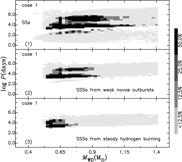
Figure 3: Gray-scale maps of WD’s mass vs. orbital period distributions for SSs and SSSs in SySs for case 1. The gradations of gray-scale correspond to the regions where the number density of systems is, respectively, within 1 – 1/2, 1/2 – 1/4, 1/4 – 1/8, 1/8 – 0 of the maximum of ${{{\partial^{2}{N}}\over{\partial{\log P}}{\partial{M_{\rm WD}}}}}$, and blank regions do not contain any stars.

Figure 3 shows the distributions of SSs and SSSs in case 1, in the “ WD’s mass – orbital period” plane. The ranges of orbital periods and WD’s masses in SSs are wider than those in SSSs. The main reason is that producing SSSs needs higher mass accretion rates and the critical ignition mass $\Delta M_{\rm crit}^{\rm WD}$ than producing SSs. As the top panel in Figure 3 shows, the distribution in SSs is cut into two regions. The low region represents these SSs which have undergone channel I, while the top region is for SSs which have undergone channels II and III.

Figure 4: Number distributions of X-ray sources in the Galactic SySs as a function of the mass accretion rate of WD (all numbers are normalized to 1). The solid, dashed and dotted lines represent SSs, SSSs from weak symbiotic novae and from steady hydrogen burning ‘ordinary’ SySs, respectively.

The distributions of numbers of X-ray sources in the Galactic SySs over the mass accretion rate of WD, $\dot{M}_{\rm acc}$, is given in Figure 4. According to our model, $\dot{M}_{\rm acc}$ determines the strength of the hydrogen burning. For low $\dot{M}_{\rm acc}$, the accreting WD experiences the strong thermonuclear outburst which results in SSs. For high $\dot{M}_{\rm acc}$, the accreting WD can undergo stable hydrogen burning. Therefore, the peaks of magnitude of $\dot{M}_{\rm acc}$ in Figure 4 are $10^{-9}$, $10^{-8}$ and $10^{-7}$$M_{\odot}\rm yr^{-1}$ for SSs, SSSs from weak symbiotic novae and from ‘ordinary’ SySs, respectively. In Iben (2003), theoretically estimated $\dot{M}_{\rm acc}$ of five SSs is between $10^{-9}$ and $10^{-8}M_{\odot}\rm yr^{-1}$, which is in good agreement with our results.

4 Conclusions

Assuming that SSs in SySs result from the violent collisions of the stellar winds during strong symbiotic novae, and SSSs from weak symbiotic novae or steady hydrogen burning SySs, we investigate the Galactic population of SSs and SSSs in SySs. The Galactic occurrence rates of SSs and SSSs are from $\sim$ 2 to 20 $\rm yr^{-1}$, and $\sim$ 2 to 17 $\rm yr^{-1}$, respectively. The numbers of X-ray sources in SySs range from 2390 to 6120. The percentage of the X-ray sources in all SySs is between $\sim$ 20% and 60%, which is in agreement with the observations.

In the present paper we do not model the X-ray spectra emissions of SSs and SSSs, and do not consider the interstellar medium’s absorptions for X-ray spectra. Our work only shows some primary results. It is necessary for a detailed model of SSs and SSSs to simulate X-ray spectra emissions and interstellar medium’s absorptions. We will consider them in the next paper.

References

- Belczyski et al. (2000) Belczyski K., Mikołajewska J., Munari U., Ivison R.J., Friedjung M., 2000, A&AS, 146, 407.
- Bergeat & Chevallier (2005) Bergeat J., Chevallier L., 2005, A&A, 429, 235.
- Formiggini et al. (1995) Formiggini L., Contini M., Leibowitz E. M., 1995, MNRAS, 277, 1071.
- Goldberg & Mazeh (1994) Goldberg D., Mazeh T., 1994, A&A, 282, 801.
- Han et al. (1995a) Han Z., Eggleton P.P., Podsiadlowski P., Tout C.A., 1995a, MNRAS, 277, 1443.
- Han et al. (1995b) Han Z., Podsiadlowski P., Eggleton P.P., 1995b, MNRAS, 272, 800.
- Hurley et al. (2002) Hurley J.R., Tout C.A., Pols R., 2002, MNRAS, 329, 897.
- Iben (2003) Iben I.Jr., 2003, ASP Conference Series, 303, 177.
- Iben & Tutukov (1996) Iben I.Jr., Tutukov A.V., 1996, ApJS, 105, 145.
- Jordan et al. (1994) Jordan S., Mürset U., Werner K., 1994, A&A, 283, 475.
- Kenyon (1986) Kenyon S.J., 1986, The Symbiotic Stars, Cambridge, Cambridge Univ.Press.
- Kenyon & Webbink (1984) Kenyon S.J., Webbink R.F., 1984, ApJ, 279, 252.
- Kraicheva et al. (1979) Kraicheva Z. T., Popova E. I., Tutukov A. V., Yungelson L. R., 1979, Soviet Astronomy, 23, 290.
- Kroupa et al. (1993) Kroupa P., Tout C.A., Gilmore G., 1993, MNRAS, 262, 545.
- Leahy & Volk (1995) Leahy D.A., Volk K., 1995, ApJ, 440, 847.
- Lü et al. (2006) Lü G.L., Yungelson L., Han Z., 2006, MNRAS, 372,1389.
- Lü et al. (2007) Lü G.L., Zhu C.H., Han Z., 2007, Chin. J. Astron. Astrophys., 7, 101.
- Lü et al. (2008) Lü G.L., Zhu C.H., Han Z., Wang Z.J., 2008, ApJ, 683, 990.
- Mazeh et al. (1992) Mazeh T., Goldberg D., Duquennoy A., Mayor M., 1992, ApJ, 401, 265.
- McCammon & Wilton (1990) McCammon D., Sanders W. T., 1990, ARA&A, 28, 657.
- Mikołajewska (2003) Mikołajewska J., 2003, in Corradi R.L.M., Mikołajewska J., Mahoney T.J., eds, ASP Conf. Ser. Vol.303, Symbiotic stars probing stellar evolution. Astron. Soc. Pac., San Francisco, p.9.
- Motch et al. (1994) Motch C., Hasinger G., Pietch W., 1994, A&A, 284, 827.
- Mürset et al. (1991) Mürset U., Nussbaumer H., Schmid H.M., Vogel M., 1991, A&A, 248, 458.
- Mürset & Schmid (1999) Mürset U., Schmid H.M., 1999, A&A, 137, 473.
- Mürset et al. (1997) Mürset U., Wolff B., Jordan S., 1997, A&A, 319, 201.
- Nelemans & Tout (2005) Nelemans G., Tout C.A., 2005, MNRAS, 356, 753.
- Nelson et al. (2004) Nelson L.A., MacCannell K.A., Dubeau E., 2004, ApJ, 602, 938.
- Nelson et al. (2008) Nelson T., Orio M., Cassinelli J. P., Still M., Leibowitz E., Mucciarelli P., 2008, ApJ, 673, 1067.
- Olofsson et al. (2002) Olofsson H., González Delgado D., Kerschbaum F., Schöier F.L., 2002, A&A, 391, 1053.
- Orlando et al. (2009) Orlando S., Drake J. J., Laming J. M., 2009, A&A, 493, 1049.
- Orio et al. (2007) Orio M., Zezas A., Munari U., Siviero A., Tepedelenlioglu E., 2007, ApJ, 661, 1105.
- Press et al. (1992) Press W. H., Teukolsky S. A., Vetterling W. T., Flannery B. P., 1992, Numerical Recipes In Fortran 77. The Art of Scientific Computing Second Edition. Cambridge Univ. Press, Combridge.
- Sokolooski et al. (2006) Sokoloski J. L., Luna G. J. M., Mukai K., Kenyon S. J., 2006, Nat., 442, 276.
- Tutukov & Yungelson (1976) Tutukov A.V., Yungelson L. R., 1976, Astrophysics, 12, 321.