Semiconjugate Factorization and Reduction of Order

in Difference Equations

H. SEDAGHAT*

Abstract. We discuss a general method by which a higher order difference equation on a group is transformed into an equivalent triangular system of two difference equations of lower orders. This breakdown into lower order equations is based on the existence of a semiconjugate relation between the unfolding map of the difference equation and a lower dimensional mapping that unfolds a lower order difference equation. Substantial classes of difference equations are shown to possess this property and for these types of equations reductions of order are obtained. In some cases a complete semiconjugate factorization into a triangular system of first order equations is possible.

1 Introduction

There are a number of known methods by which a difference equation can be transformed into equations with lower orders. These methods are almost universally adapted from the theory of differential equations and can be divided into two major categories. One category uses symmetries in the solutions of a difference equation to obtain coordinate transformations that lead to a reduction in order; see, e.g., [3], [10], [13], [14]. The second category consists of methods (e.g., operator methods) that rely on the algebraic and analytical properties of the difference equation itself; see, e.g., [7], [11]. For historical reasons the first of these categories has been developed considerably more than the second.

In this article we introduce a general new method that falls into the second category. This method uses the existence of a semiconjugate relation to break down a given difference equation into an equivalent pair of lower order equations whose orders add up to the order of the original equation. A salient feature of the equivalent system of two equations is its “triangular” nature; see [1] for a formal definition as well as a study of the periodic structure of solutions. Also see [26] for additional information and a list of references. Such a system is uncoupled in the sense that one of the two equations is independent of the other.

In some cases (e.g., linear equations) we use the semiconjugate relation repeatedly to transform a higher order difference equation into an equivalent system of first order equations with triangular uncoupling. In the specific case of linear equations, the system of first order equations explicitly reveals all of the eigenvalues of the higher order equation.

Semiconjugate-based reduction in order uses only patterns or symmetries inherent in the form of the difference equation itself. For this reason, we do not limit ourselves to equations defined on real numbers. Allowing more general types of objects not only improves the applicability of the method to areas where discrete modeling naturally occurs (e.g., dynamics on networks, see for instance, [15]) but it is actually helpful in identifying form symmetries even within the context of real numbers where more than one algebraic operation is defined. After defining the basic idea of semiconjugate factorization and laying some groundwork we discuss applications of the method to reduction of order in several classes of difference equations.

2 Difference equations and semiconjugacy

Difference equations of order greater than one that are of the following type

$$x_{n+1}=f_{n}(x_{n},x_{n-1},\ldots,x_{n-k})$$ (1)

determine the forward evolution of a variable $x_{n}$ in discrete time. As is customary, the time index or the independent variable $n$ is integer-valued, i.e., $n\in\mathbb{Z}$. The number $k$ is a fixed positive integer and $k+1$ represents the order of the difference equation (1). If the underlying space of variables $x_{n}$ is labled $G$ then $f_{n}:G^{k+1}\rightarrow G$ is a given function for each $n\geq 1$. If $f_{n}=f$ does not explicitly depend on $n$ then (1) is said to be autonomous. A solution of Eq.(1) is any function $x:\mathbb{Z}\rightarrow G$ that satisfies the difference equation. A forward solution is a sequence $\{x_{n}\}_{n=-k}^{\infty}$ that is recursively generated by (1) from a set of $k+1$ initial values $x_{0},x_{-1},\ldots,x_{-k}\in G.$ Forward solutions have traditionally been of greater interest in discrete models that are based on Eq.(1).

If the functions $f_{n}$ do not have any singularities in $G$  for all $n$ then clearly the existence of forward solutions is guaranteed from any given set of initial values. Otherwise, sets of initial values that upon a finite number of iterations lead to a singularity of $f_{n}$ for some $n$ must either be specified or avoided. In this paper we do not discuss the issue of singularities broadly but deal with them as they occur in various examples.

We assume that the underlying space $G$ of variables $x_{n}$ is endowed with an algebraic group structure; for a study of semiconjugacy in a topological context see [24] or [25]. Often there are multiple group operations defined on a given set $G$. This feature turns out to be quite useful. Compatible topologies (making group operation(s) continuous) may exist on $G$ and often occur in applications. Topological or metric concepts may be used explicitly in defining certain form symmetries and are required in discussing the asymptotic behaviors of solutions with unknown closed forms in infinite sets.

We “unfold” each $f_{n}$ in the usual way using the functions $F_{n}:G^{k+1}\rightarrow G^{k+1}$ defined as

$$F_{n}(u_{0},\ldots,u_{k})=[f_{n}(u_{0},\ldots,u_{k}),u_{0},\ldots,u_{k-1}],\quad u_{j}\in G\text{ for }j=0,1,\ldots,k.$$ (2)

The unfoldings (or associated vector maps) $F_{n}$ determine the equation

$$(y_{0,n+1},y_{1,n+1},\ldots,y_{k,n+1})=F_{n}(y_{0,n},y_{1,n},\ldots,y_{k,n})$$

in $G^{k+1}$ or equivalently, the system of equations

$$y_{j,n+1}=\left\{\begin{array}[c]{l}f_{n}(y_{0,n},y_{1,n},\ldots,y_{k,n}),\text{ if }j=0\\ y_{j-1,n},\text{ for }j=1,\ldots,k\end{array}\right..$$

In this context we refer to $(y_{0,n},y_{1,n},\ldots,y_{k,n})$ as the state of the system at time $n$ and to $G^{k+1}$ as the state space of the system, or of (1).

Definition 1

Let $S$ and $M$ be arbitrary nonempty sets and let $F,\Phi$ be self maps of $S$ and $M$, respectively. If there is a surjective (onto) mapping $H:S\rightarrow M$ such that

$$H\circ F=\Phi\circ H$$ (3)

then we say that the mapping $F$ is semiconjugate to $\Phi$ and write $F\trianglerighteq\Phi$. We refer to $\Phi$ as a semiconjugate (SC) factor of $F$. The function $H$ may be called a link map. If $H$ is a bijection (one to one and onto) then we call $F$ and $\Phi$ conjugates and alternatively write

$$\Phi=H\circ F\circ H^{-1}.$$ (4)

We use the notation $F\simeq\Phi$ when $F$ and $\Phi$ are conjugates. Straightforward arguments show that $\simeq$ is an equivalence relation for self maps and that $\trianglerighteq$ is a transitive relation.

As our first example shows, the fact that the link map $H$ is not injective or one-to-one is essential for reduction of order. Such a non-conjugate map often exists where conjugacy does not.

Example 2

Consider the following self maps of the plane $\mathbb{R}^{2}$:

$$F_{1}(u,v)=[u^{2}+v^{2},2uv],\quad F_{2}(u,v)=[u^{2}-v^{2},2uv].$$

Note that $u^{2}+v^{2}+2uv=(u+v)^{2}$ so let $H_{1}(u,v)=u+v$ to obtain

$$H_{1}(F_{1}(u,v))=(u+v)^{2}=[H_{1}(u,v)]^{2}.$$

It follows that $F_{1}$ is semiconjugate to $\Phi(t)=t^{2}$ on $\mathbb{R}.$ For $F_{2}$ define $H_{2}(u,v)=(u^{2}+v^{2})^{1/2}$ to get

$$H_{2}(F_{2}(u,v))=\sqrt{\left(u^{2}-v^{2}\right)^{2}+4u^{2}v^{2}}=u^{2}+v^{2}=[H_{2}(u,v)]^{2}.$$

Therefore, $F_{2}$ is also semiconjugate to $\Phi(t)=t^{2}$ though this time on $[0,\infty)$ since $H_{2}(u,v)\geq 0$ for all $(u,v)\in$ $\mathbb{R}^{2}$.

In the next example we determine all possible semiconjugates for a difference equation on a finite field.

Example 3

Consider the following autonomous difference equation of order 2 on $\mathbb{Z}_{2}=\{0,1\}$

$$x_{n+1}=(x_{n}+1)x_{n-1},\quad x_{0},x_{-1}\in\{0,1\}$$

Note that $\mathbb{Z}_{2}$ is a field under addition modulo 2 and ordinary multiplication of integers. The unfolding of the defining map $f(u,v)=(u+1)v$ is given by $F(u,v)=[(u+1)v,u]$. In order to determine the semiconjugates of $F$ on $\mathbb{Z}_{2}^{2}$ first we list the four possible self maps of $\mathbb{Z}_{2}$, i.e.,

$$\phi_{0} \equiv 0,\quad\phi_{1}\equiv 1\quad\text{(constant functions)}$$

$$\iota(t) =t\quad\text{(the identity function)}$$

$$\phi(t) =t+1.$$

Next, there are 16 link maps $H:\mathbb{Z}_{2}^{2}\rightarrow\mathbb{Z}_{2}$ of which the 14 non-constant ones are surjective. We list these 14 maps succinctly as follows:

$$\begin{array}[c]{cccc}H_{1}=(0,0,0,1)&H_{2}=(0,0,1,0)&H_{3}=(0,0,1,1)&H_{4}=(0,1,0,0)\\ H_{5}=(0,1,0,1)&H_{6}=(0,1,1,0)&H_{7}=(0,1,1,1)&H_{8}=(1,0,0,0)\\ H_{9}=(1,0,0,1)&H_{10}=(1,0,1,0)&H_{11}=(1,0,1,1)&H_{12}=(1,1,0,0)\\ H_{13}=(1,1,0,1)&H_{14}=(1,1,1,0)&&\end{array}$$

In the above list, for instance $H_{14}$ is defined by the rule

$$H_{14}:(0,0)\rightarrow 1,\ (0,1)\rightarrow 1,\ (1,0)\rightarrow 1,\ (1,1)\rightarrow 0$$

and can be written in algebraic form as $H_{14}(u,v)=uv+1.$ The other link maps are defined in the same way. Now writing $F$ as

$$F:(0,0)\rightarrow(0,0),\ (0,1)\rightarrow(1,0),\ (1,0)\rightarrow(0,1),\ (1,1)\rightarrow(0,1)$$

and calculating the compositions $H_{j}\circ F$ for $j=1,\ldots,14$ the following results are obtained:

$$H_{1}\circ F =(0,0,0,0)=\phi_{0}\circ H_{1},\quad H_{14}\circ F=(1,1,1,1)=\phi_{1}\circ H_{14}$$

$$H_{7}\circ F =(0,1,1,1)=H_{7}\circ\iota,\quad H_{8}\circ F=(1,0,0,0)=H_{8}\circ\iota.$$

Therefore, $F$ is semiconjugate to each of $\phi_{0},\phi_{1}$ and $\iota$ but not to $\phi$ (but also see Example 7 below).

It is worth noting that the maps $H_{7}$ and $H_{8}$ are invariants (see, e.g., [2], [9], [16]) because the factor map is the identity function ($\iota$ here). It is easy to check that in algebraic form the two invariants can be written as

$$H_{7}(u,v)=uv+u+v,\quad H_{8}(u,v)=uv+u+v+1=(u+1)(v+1).$$

3 Semiconjugate factorization

In this section we define the concepts needed to present our results in subsequent sections.

3.1 Form symmetries, factors and cofactors

To make the transition from semiconjugate maps to reduction of order in difference equations, let $k$ be a non-negative integer and $G$ a nonempty set. Let $\{F_{n}\}$ be a family of functions $F_{n}:G^{k+1}\rightarrow G^{k+1}$ where $F_{n}=[f_{1,n},\ldots,f_{k+1,n}]$  and $f_{j,n}:G\rightarrow G$ are the component functions of $F_{n}$ for all $j$ and all $n.$

Let $m$ be an integer, $1\leq m\leq k+1$ and assume that each $F_{n}$ is semiconjugate to a map $\Phi_{n}:G^{m}\rightarrow G^{m}$. Let $H:G^{k+1}\rightarrow G^{m}$ be the link map such that for every $n,$

$$H\circ F_{n}=\Phi_{n}\circ H.$$ (5)

Suppose that

$$H(u_{0},\ldots,u_{k}) =[h_{1}(u_{0},\ldots,u_{k}),\ldots,h_{m}(u_{0},\ldots,u_{k})]$$

$$\Phi_{n}(t_{1},\ldots,t_{m}) =[\phi_{1,n}(t_{1},\ldots,t_{m}),\ldots,\phi_{m,n}(t_{1},\ldots,t_{m})]$$

where $h_{j}:G^{k+1}\rightarrow G$ and $\phi_{j,n}:G\rightarrow G$ are the corresponding component functions for $j=1,2,\ldots,m$. Then identity (5) is equivalent to the system of equations

$$h_{j}(f_{1,n}(u_{0},\ldots,u_{k}),\ldots,f_{k+1,n}(u_{0},\ldots,u_{k}))=$$

$$\phi_{j,n}(h_{1}(u_{0},\ldots,u_{k}),\ldots,h_{m}(u_{0},\ldots,u_{k})),\quad j=1,2,\ldots,m.$$ (6)

If the functions $f_{j,n}$ are given then (6) is a system of functional equations whose solutions $h_{j},\phi_{j,n}$ give the maps $H$ and $\Phi_{n}.$ Note that if $m<k+1$ then the functions $\Phi_{n}$ on $G^{m}$ define a system with lower dimension than that defined by the functions $F_{n}$ on $G^{k+1}.$ We now proceed to find a solution set for (6).

Let $G$ be a group and denote its operation by $\ast.$ If $F_{n}$ is the unfolding of the function $f_{n}$ as in (2) and $F_{n}$ satisfies (5) then it need not follow that the maps $\Phi_{n}$ are of scalar type similar to $F_{n}.$ To ensure that each $\Phi_{n}$ is also of scalar type we define the first component function of $H$ as

$$h_{1}(u_{0},\ldots,u_{k})=u_{0}\ast h(u_{1},\ldots,u_{k})$$ (7)

where $h:G^{k}\rightarrow G$ is a function to be determined.

Using (7) in the first equation in (6) gives

$$f_{n}(u_{0},\ldots,u_{k})\ast h(u_{0},\ldots,u_{k-1})=$$ (8)

$$g_{n}(u_{0}\ast h(u_{1},\ldots,u_{k}),h_{2}(u_{0},\ldots,u_{k}),\ldots,h_{m}(u_{0},\ldots,u_{k}))$$

where the abbreviation $g_{n}$ is used for $\phi_{1,n}:G^{m}\rightarrow G.$

Eq.(8) is a functional equation in which the functions $h,h_{j},g_{n}$ may be determined in terms of the given functions $f_{n}$. Our aim is to extract a scalar equation of order $m$ such as

$$t_{n+1}=g_{n}(t_{n},\ldots,t_{n-m+1})$$ (9)

from (8) in such a way that the maps $\Phi_{n}$ will be of scalar type. The basic framework for carrying out this process is already in place; let $\{x_{n}\}$ be a solution of Eq.(1) and define

$$t_{n}=x_{n}\ast h(x_{n-1},\ldots,x_{n-k}).$$

Then the left hand side of (8) is

$$x_{n+1}\ast h(x_{n},\ldots,x_{n-k+1})=t_{n+1}.$$ (10)

which gives the initial part of the difference equation (9). In order that the right hand side of (8) coincide with that in (9) it is necessary to define the component functions in (8) as

$$h_{j}(x_{n},\ldots,x_{n-k}) =t_{n-j+1}=x_{n-j+1}\ast h(x_{n-j},\ldots,x_{n-k-j+1}),$$ (11)

$$\text{for }j =2,\ldots,m.$$

Since the left hand side of (11) does not depend on the terms

$$x_{n-k-1},\ldots,x_{n-k-j+1}$$

it follows that the function $h_{j}$ must be constant in its last few coordinates. Since $h$ does not depend on $j,$ the number of its constant coordinates is found from the last function $h_{m}.$ Specifically, we have

$$h_{m}(x_{n},\ldots,x_{n-k})=x_{n-m+1}\ast h(\underset{k-m+1\text{ variables}}{\underbrace{x_{n-m},\ldots,x_{n-k}}},\underset{m-1\text{ terms with }h\text{ constant}}{\underbrace{x_{n-k-1},\ldots,x_{n-k-m+1}}})$$ (12)

The preceding condition leads to the necessary restrictions on $h$ and every $h_{j}$ for a consistent derivation of (9) from (8). Therefore, (12) is a consistency condition. Now from (11) and (12) we obtain for $(u_{0},\ldots,u_{k})\in G^{k+1}$

$$h_{j}(u_{0},\ldots,u_{k})=u_{j-1}\ast h(u_{j},u_{j+1}\ldots,u_{j+k-m}),\quad j=1,\ldots,m.$$ (13)

With this definition for the coordinate functions $h_{j}$ we rewrite (8) for later reference as

$$f_{n}(u_{0},\ldots,u_{k})\ast h(u_{0},\ldots,u_{k-m})=$$

$$g_{n}(u_{0}\ast h(u_{1},\ldots,u_{k-m+1}),u_{1}\ast h(u_{2},\ldots,u_{k-m+2}),\ldots,u_{m-1}\ast h(u_{m},\ldots,u_{k}))$$ (14)

We now define a natural form symmetry concept for the recursive difference equation (1).

Definition 4

The function $H=[h_{1},\ldots,h_{m}]$ whose components $h_{j}$ are defined by (13) is a (recursive) form symmetry for Eq.(1). Since the range of $H$ has a lower dimension $m$ than the dimension $k+1$ of its domain, we say that $H$ is an order-reducing form symmetry.

For each solution $\{x_{n}\}$ of (1) according to (8), (10) and (13) the sequence

$$t_{n}=x_{n}\ast h(x_{n-1},\ldots,x_{n-k+m-1})$$

is a solution of (9) with initial values

$$t_{-j}=x_{-j}\ast h(x_{-j-1},\ldots,x_{-j-k+m-1}),\quad j=0,\ldots,m-1.$$ (15)

Thus, the following pair of lower order equations are satisfied:

$$t_{n+1} =g_{n}(t_{n},\ldots,t_{n-m+1}),$$ (16)

$$x_{n+1} =t_{n+1}\ast[h(x_{n},\ldots,x_{n-k+m})]^{-1}$$ (17)

where $-1$ denotes group inversion in $G.$ The pair of equations (16) and (17) is uncoupled in the sense that (16) is independent of (17). Such a pair forms a triangular system as defined in [1] and [26].

Definition 5

Eq.(16) is a factor of Eq.(1) since it is derived from the semiconjugate factor $\Phi_{n}.$ Eq.(17) that links the factor to the original equation is a cofactor of Eq.(1). We refer to the system of equations (16) and (17) as a semiconjugate (SC) factorization of Eq.(1). Note that orders $m$ and $k+1-m$ of (16) and (17) respectively, add up to the order of (1).

3.2 The factorization theorem

We are now ready for the following fundamental result, i.e., the equivalence of Eq.(1) with the system of equations (16) and (17).

Theorem 6

Let $k\geq 1$, $1\leq m\leq k$ and suppose that there are functions $h:G^{k-m+1}\rightarrow G$ and $g_{n}:G^{m}\rightarrow G$ that satisfy equations (8) and (13).

(a) With the order-reducing form symmetry

$$H(u_{0},\ldots,u_{k})=[u_{0}\ast h(u_{1},\ldots,u_{k+1-m}),\ldots,u_{m-1}\ast h(u_{m},\ldots,u_{k})]$$ (18)

Eq.(1) is equivalent to the SC factorization consisting of the triangular system of equations (16) and (17).

(b) The function $H:G^{k+1}\rightarrow G^{m}$ defined by (18) is surjective.

(c) For each $n$, the SC factor map $\Phi_{n}:G^{m}\rightarrow G^{m}$ in (5) is the unfolding of Eq.(16). In particular, each $\Phi_{n}$ is of scalar type.

Proof. (a) To show that the SC factorization system consisting of equations (16) and (17) is equivalent to Eq.(1) we show that: (i) each solution $\{x_{n}\}$ of (1) uniquely generates a solution of (16) and (17) and conversely (ii) each solution $\{(t_{n},y_{n})\}$ of the system (16) and (17) correseponds uniquely to a solution $\{x_{n}\}$ of (1). To establish (i), let $\{x_{n}\}$ be the unique solution of (1) corresponding to a given set of initial values $x_{0},\ldots x_{-k}\in G.$ Define the sequence

$$t_{n}=x_{n}\ast h(x_{n-1},\ldots,x_{n-k+m-1})$$ (19)

for $n\geq-m+1.$ Then for each $n\geq 0$ using (14)

$$x_{n+1} =f_{n}(x_{n},\ldots,x_{n-k})$$

$$=g_{n}(x_{n}\ast h(x_{n-1},\ldots,x_{n-k+m-1}),\ldots,x_{n-m+1}\ast h(x_{n-m},\ldots,x_{n-k}))\ast$$

$$\hskip 216.81pt[h(x_{n},\ldots,x_{n-k+m})]^{-1}$$

$$=g_{n}(t_{n},\ldots,t_{n-m+1})\ast[h(x_{n},\ldots,x_{n-k+m})]^{-1}$$

Therefore, $g_{n}(t_{n},\ldots,t_{n-m+1})=x_{n+1}\ast h(x_{n},\ldots,x_{n-k+m})=t_{n+1}$ so that $\{t_{n}\}$ is the unique solution of the factor equation (16) with initial values

$$t_{-j}=x_{-j}\ast h(x_{-j-1},\ldots,x_{-j-k+m-1}),\quad j=0,\ldots,m-1.$$

Further, by (19) for $n\geq 0$ we have $x_{n+1}=t_{n+1}\ast[h(x_{n},\ldots,x_{n-k+m})]^{-1}$ so that $\{x_{n}\}$ is the unique solution of the cofactor equation (17) with initial values $y_{-i}=x_{-i}$ for $i=0,1,\ldots,k-m$ and $t_{n}$ as obtained above.

To establish (ii), let $\{(t_{n},y_{n})\}$ be a solution of the factor-cofactor system with initial values

$$t_{0},\ldots,t_{-m+1},y_{-m},\ldots y_{-k}\in G.$$

Note that these numbers determine $y_{-m+1},\ldots,y_{0}$ through the cofactor equation

$$y_{-j}=t_{-j}\ast[h(y_{-j-1},\ldots,y_{-j-1-k+m})]^{-1},\quad j=0,\ldots,m-1.$$ (20)

Now using (14) for $n\geq 0$ we obtain

$$y_{n+1} =t_{n+1}\ast[h(y_{n},\ldots,y_{n-k+m})]^{-1}$$

$$=g_{n}(t_{n},\ldots,t_{n-m+1})\ast[h(y_{n},\ldots,y_{n-k+m})]^{-1}$$

$$=g_{n}(y_{n}\ast h(y_{n-1},\ldots,y_{n-k+m-1}),\ldots,y_{n-m+1}\ast h(y_{n-m},\ldots,y_{n-k}))\ast$$

$$\hskip 216.81pt[h(y_{n},\ldots,y_{n-k+m})]^{-1}$$

$$=f_{n}(y_{n},\ldots,y_{n-k})$$

Thus $\{y_{n}\}$ is the unique solution of Eq.(1) that is generated by the initial values (20) and $y_{-m},\ldots y_{-k}.$ This completes the proof of (a).

(b) Choose an arbitrary point $[v_{1},\ldots,v_{m}]\in G^{m}$ and set

$$u_{m-1}=v_{m}\ast h(u_{m},u_{m+1}\ldots,u_{k})^{-1}$$

where $u_{m}=u_{m+1}=\ldots u_{k}=\bar{u}$ where $\bar{u}$ is a fixed element of $G,$ e.g., the identity. Then

$$v_{m} =u_{m-1}\ast h(\bar{u},\bar{u}\ldots,\bar{u})$$

$$=u_{m-1}\ast h(u_{m},u_{m+1}\ldots,u_{k})$$

$$=h_{m}(u_{0},\ldots,u_{k})$$

$$=h_{m}(u_{0},\ldots,u_{m-2},v_{m}\ast h(\bar{u},\bar{u}\ldots,\bar{u})^{-1},\bar{u}\ldots,\bar{u}).$$

for any choice of points $u_{0},\ldots,u_{m-2}\in G.$ Similarly, define

$$u_{m-2}=v_{m-1}\ast h(u_{m-1},u_{m}\ldots,u_{k-1})^{-1}$$

so as to get

$$v_{m-1} =u_{m-2}\ast h(u_{m-1},u_{m}\ldots,u_{k-1})$$

$$=h_{m-1}(u_{0},\ldots,u_{k})$$

$$=h_{m-1}(u_{0},\ldots,u_{m-3},v_{m-1}\ast h(u_{m-1},\bar{u}\ldots,\bar{u})^{-1},u_{m-1},\bar{u}\ldots,\bar{u})$$

for any choice of $u_{0},\ldots,u_{m-3}\in G.$ Continuing in this way, induction leads to selection of $u_{m-1},\ldots,u_{0}$ such that

$$v_{j}=h_{j}(u_{0},\ldots,u_{m-1},\bar{u}\ldots,\bar{u}),\quad j=1,\ldots,m.$$

Therefore, $H(u_{0},\ldots,u_{m-1},\bar{u}\ldots,\bar{u})=[v_{1},\ldots,v_{m}]$ and it follows that $H$ is onto $G^{m}.$

(c) It is necessary to prove that each coordinate function $\phi_{j,n}$ is the projection into coordinate $j-1$ for $j>1.$ Suppose that the maps $h_{j}$ are given by (13). For $j=2$ (6) gives

$$\phi_{2,n}(h_{1}(u_{0},\ldots,u_{k}),\ldots,h_{m}(u_{0},\ldots,u_{k})) =h_{2}(f_{n}(u_{0},\ldots,u_{k}),u_{0},\ldots,u_{k-1})$$

$$=u_{0}\ast h(u_{1},u_{2}\ldots,u_{k-m+1})$$

$$=h_{1}(u_{0},\ldots,u_{k}).$$

Therefore, $\phi_{2,n}$ projects into coordinate 1. Generally, for $j\geq 2$ we have

$$\phi_{j,n}(h_{1}(u_{0},\ldots,u_{k}),\ldots,h_{m}(u_{0},\ldots,u_{k})) =h_{j}(f_{n}(u_{0},\ldots,u_{k}),u_{0},\ldots,u_{k-1})$$

$$=u_{j-2}\ast h(u_{j-1},u_{j}\ldots,u_{j+k-m-1})$$

$$=h_{j-1}(u_{0},\ldots,u_{k}).$$

Therefore, for each $n$ and for every $(t_{1},\ldots,t_{m})\in H(G^{k+1})$ we have

$$\Phi_{n}(t_{1},\ldots,t_{m})=[g_{n}(t_{1},\ldots,t_{m}),t_{1},\ldots,t_{m-1}]$$

i.e., $\Phi_{n}|_{H(G^{k+1})}$ is of scalar type. Since by Part (b) $H(G^{k+1})=G^{m}$ it follows that $\Phi_{n}$ is of scalar type.   

We point out that the SC factorization in Theorem 6(a) does not require the determination of $\phi_{j,n}$ for $j\geq 2.$ However, as seen in Parts (b) and (c) of the theorem the rest of the picture fits together properly.

We discuss several applications of Theorem 6 in later sections below. The following example gives an application in finite settings.

Example 7

Let $G$ be any nontrivial abelian group (e.g., $\mathbb{Z}_{2}$ in Example 3 viewed as an additive group) and consider the following difference equation of order two

$$x_{n+1}=x_{n-1}+a,\quad a,x_{0},x_{-1}\in G,\ a\not=0.$$ (21)

The unfolding of Eq.(21) is the map $F(u,v)=[v+a,u].$ Note that the function $H(u,v)=u+v$ is of type $u+h(v)$ with $h$ being the identity function on $G$ ($H$ is the same as $H_{6}$ in Example 3). With this $H$ we have

$$H(F(u,v))=u+v+a=\phi(H(u,v))$$

where $\phi:G\rightarrow G$ is defined as $\phi(t)=t+a$. Therefore, $F\trianglerighteq\phi.$ Using Theorem 6 we obtain the SC factorization of Eq.(21) as

$$t_{n+1} =\phi(t_{n})=t_{n}+a,\ t_{0}=H(x_{0},x_{-1})=x_{0}+x_{-1}$$

$$x_{n+1} =t_{n+1}-x_{n}=t_{n+1}+x_{n}.$$

3.3 Reduction types and chains

Theorem 6 leads to a natural classification scheme for order reduction which we discuss in this section. We begin with a definition.

Definition 8

The SC factorization of Eq.(1) into (16) and (17) gives a type-($m,k+1-m$) order reduction (or just type-($m,k+1-m$) reduction) for (1). We also say that (1) is a type-($m,k+1-m$) equation in this case.

A second-order difference equation ($k=1$) can have only the type-(1,1) order reduction into two first order equations. A third-order equation has two order reduction types, namely (1,2) and (2,1), a fourth order equation has three order reduction types (1,2), (2,2) and (2,1) and so on. Of the $k$ possible order reduction types

$$(1,k),\ (2,k-1),\cdots,(k-1,2),\ (k,1)$$

for an equation of order $k+1$ the two extreme ones, namely $(1,k)$ and $(k,1)$ have the extra appeal of having an equation of order 1 as either a factor or a cofactor.

Eq.(1) may admit repeated reductions of order through its factor equation, its cofactor equation or both as follows:

$$\text{Eq.(\ref{dek})}\rightarrow\left\{\begin{array}[c]{ll}\underset{\text{factor equation}}{\underbrace{t_{n+1}=g_{n}(t_{n},\ldots,t_{n-m+1})}}\quad\rightarrow&\left\{\begin{array}[c]{l}\text{factor\ }\rightarrow\cdots\\ \text{cofactor }\rightarrow\cdots\end{array}\right.\\ \underset{\text{cofactor equation}}{\underbrace{x_{n+1}=t_{n+1}\ast h(x_{n},\ldots,x_{n-k+m})^{-1}}}\,\rightarrow&\left\{\begin{array}[c]{l}\text{factor }\rightarrow\cdots\\ \text{cofactor }\rightarrow\cdots\end{array}\right.\end{array}\right.$$

In the above binary tree structure, we call each branch a reduction chain. If a reduction chain consists only of factor (or cofactor) equations then it is a factor (or cofactor) chain. In particular, we show later (Corollary 20 below) that a linear difference equation of order $k+1$ has a full cofactor chain leading to a system of $k+1$ linear first order equations, as discussed earlier in the introduction. The next example exhibits a full factor chain.

Example 9

Consider the following reduction chain:

$$x_{n+1}=x_{n}+\frac{a(x_{n}-x_{n-1})^{2}}{x_{n-1}-x_{n-2}}\rightarrow\left\{\begin{array}[c]{ll}t_{n+1}=\dfrac{at_{n}^{2}}{t_{n-1}}\ \rightarrow&\left\{\begin{array}[c]{l}s_{n+1}=as_{n}\\ t_{n+1}=s_{n+1}t_{n}\end{array}\right.\\ x_{n+1}=t_{n+1}+x_{n}&\end{array}\right.$$ (22)

The 3rd order equation is reduced by substituting $t_{n}=x_{n}-x_{n-1}$, then the 2nd order factor equation is reduced by the substitution $s_{n}=t_{n}/t_{n-1}$ (see Definition 13 below and the comments that follow it). The factor chain in this example has length three as follows:

$$x_{n+1}=x_{n}+\frac{a(x_{n}-x_{n-1})^{2}}{x_{n-1}-x_{n-2}}\rightarrow t_{n+1}=\dfrac{at_{n}^{2}}{t_{n-1}}\rightarrow s_{n+1}=as_{n}.$$

Since a first order difference equation does not have order-reducing form symmetries the SC factorization process of an equation of order $k+1$ must stop in at most $k$ steps. The result then is a system of $k+1$ first order equations that mark the ends of factor/cofactor chains. In (22) the three first order equations that mark the ends of factor/cofactor chains can be arranged as follows:

$$s_{n+1} =as_{n}$$

$$t_{n+1} =as_{n}t_{n}$$ (23)

$$x_{n+1} =as_{n}t_{n}+x_{n}.$$

Since each equation depends on the variables in the equations above it, (23) is a “triangular system.” In principle, a triangular system can be solved by solving the top-most equation and then using that solution to solve the next equation and so on. In the case of (23) since the equations are linear (including the nonautonomous and nonhomogenous versions) an explicit formula for solutions of the system can be determined; in particular, the third order equation (22) is integrable. Whether a complete SC factorization as a triangular system exists for each higher order difference equation of type (1) is a difficult question that is equivalent to the apparently more basic problem of existence of semiconjugate relations for (1).

4 Reduction of order of difference equations

In this section we use the methods of the previous section to obtain reductions in orders of various classes of difference equations.

4.1 Equations with type-$(k,1)$ reductions

For type-$(k,1)$ reductions of Eq.(1) $m=k$. Therefore, the function $h:G\rightarrow G$ in (13) is of one variable and yields the form symmetry

$$H(u_{0},\ldots,u_{k})=[u_{0}\ast h(u_{1}),u_{1}\ast h(u_{2})\ldots,u_{k-1}\ast h(u_{k})].$$ (24)

Theorem 6 gives the SC factorization as the pair

$$t_{n+1} =g_{n}(t_{n},t_{n-1},\ldots,t_{n-k+1})$$ (25)

$$x_{n+1} =t_{n+1}\ast[h(x_{n})]^{-1}.$$ (26)

The functions $g_{n}:G^{k}\rightarrow G$ are determined by the given functions $f_{n}$ in (1) as in the previous sections. From the semiconjugate relation it follows that a type-($k,1$) reduction with a form symmetry of type (24) exists if and only if there are functions $g_{n}$ such that

$$g_{n}(u_{0}\ast h(u_{1}),u_{1}\ast h(u_{2}),\ldots,u_{k-1}\ast h(u_{k}))=f_{n}(u_{0},u_{1},\ldots,u_{k})\ast h(u_{0}).$$ (27)

Remark 1. The order of the factor equation (25) is one less than the order of (1). If a solution $t_{n+1}$ of (25) is known then by the factorization theorem the corresponding solution $x_{n}$ of (1) is obtained by solving the cofactor equation (26), which has order one. For this reason we may refer to Eq.(25) as an order reduction for Eq.(1).

4.1.1 Invertibility criterion

The next result from [19] gives a necessary and sufficient condition for the existence of $\phi_{n}$ when the function $h$ above is invertible. We repeat the proof for the reader’s convenience.

Notation: the symbol $h^{-1}(\cdot)$ denotes the inverse of $h$ as a function and the symbol $h(\cdot)^{-1}$ denotes group inversion.

Theorem 10

(Invertibility criterion) Let $h:G\rightarrow G$ be a bijection. For $u_{0},v_{1},\ldots,v_{k}\in G$ let $\zeta_{0}=u_{0}$ and define

$$\zeta_{j}=h^{-1}(\zeta_{j-1}^{-1}\ast v_{j}),\quad j=1,\ldots,k.$$ (28)

Then Eq.(1) has the form symmetry (24) with SC factors $\phi_{n}$ satisfying (27) if and only if the quantity

$$f_{n}(u_{0},\zeta_{1},\ldots,\zeta_{k})\ast h(u_{0})$$ (29)

is independent of $u_{0}$ for every $n$.

Proof. First assume that the quantity in (29) is independent of $u_{0}$ for all $v_{1},\ldots,v_{k}$ so that the function

$$g_{n}(v_{1},\ldots,v_{k})=f_{n}(u_{0},\zeta_{1},\ldots,\zeta_{k})\ast h(u_{0})$$ (30)

is well defined. Next, if $H$ is given by (24) then for all $u_{0},u_{1},\ldots,u_{k}$

$$g_{n}(H(u_{0},u_{1},\ldots,u_{k}))=g_{n}(u_{0}\ast h(u_{1}),u_{1}\ast h(u_{2}),\ldots,u_{k-1}\ast h(u_{k})).$$

Define

$$v_{j}=u_{j-1}\ast h(u_{j}),\quad j=1,\ldots,k.$$ (31)

Then by (28)

$$\zeta_{1}=h^{-1}(u_{0}^{-1}\ast v_{1})=h^{-1}(u_{0}^{-1}\ast u_{0}\ast h(u_{1}))=u_{1}.$$

In fact $\zeta_{j}=u_{j}$ for every $j,$ for if by way of induction $\zeta_{l}=u_{l}$ for $1\leq l<j$ then

$$\zeta_{j}=h^{-1}(\zeta_{j-1}^{-1}\ast v_{j})=h^{-1}(u_{j-1}^{-1}\ast u_{j-1}\ast h(u_{j}))=u_{j}.$$

Now by (30)

$$g_{n}(H(u_{0},u_{1},\ldots,u_{k}))=f_{n}(u_{0},\ldots,u_{k})\ast h(u_{0})$$

so if $F_{n}$ and $\Phi_{n}$ are the unfoldings of $f_{n}$ and $g_{n}$ respectively, then

$$H(F_{n}(u_{0},\ldots,u_{k})) =[f_{n}(u_{0},\ldots,u_{k})\ast h(u_{0}),u_{0}\ast h(u_{1}),\ldots,u_{k-2}\ast h(u_{k-1})]$$

$$=[g_{n}(H(u_{0},u_{1},\ldots,u_{k})),u_{0}\ast h(u_{1}),\ldots,u_{k-2}\ast h(u_{k-1})]$$

$$=\Phi_{n}(H(u_{0},\ldots,u_{k}))$$

Finally, to show that $H$ is a semiconjugate link for Eq.(1) we show that $H$ is onto $G^{k}.$ Let $(v_{1},\ldots,v_{k})\in G^{k}$ and let $u_{k}$ be any element of $G,$ e.g., the identity. Define

$$u_{j-1}=v_{j}\ast[h(u_{j})]^{-1},\quad j=k,k-1,\ldots,1$$

and note that

$$H(u_{0},\ldots,u_{k}) =[u_{0}\ast h(u_{1}),u_{1}\ast h(u_{2})\ldots,u_{k-1}\ast h(u_{k})]$$

$$=[v_{1},v_{2},\ldots,v_{k}]$$

i.e., $H$ is onto $G^{k}$ as claimed.

Conversely, if $H$ as given by (24) is a form symmetry then the semiconjugate relation implies that there are functions $g_{n}$ such that

$$f_{n}(u_{0},\ldots,u_{k})\ast h(u_{0})=g_{n}(u_{0}\ast h(u_{1}),\ldots,u_{k-1}\ast h(u_{k})).$$ (32)

For every $v_{1},\ldots,v_{k}$ in $G$ and with $\zeta_{j}$ as defined in (28),

$$f_{n}(u_{0},\zeta_{1},\ldots,\zeta_{k})\ast u_{0} =g_{n}(u_{0}\ast h(\zeta_{1}),\zeta_{1}\ast h(\zeta_{2}),\ldots,\zeta_{k-1}\ast h(\zeta_{k}))$$

$$=g_{n}(v_{1},\ldots,v_{k})$$

which is clearly independent of $u_{0}.$   

It is worth noting that (28) is a backwards version of the cofactor equation (26) that is obtained by solving it for $x_{n}$ instead of $x_{n+1}.$ To do this we required $h$ to be invertible. Of course, in (28) it is necessary to iterate only $k$ times.

4.1.2 Identity and inversion form symmetries

We now examine two of the simplest possible form symmetries within the context of the previous section that are based on the scalar maps

$$h_{1}(u)=u\quad\text{and}\quad h_{-1}(u)=u^{-1}.$$

Each of $h_{\pm 1}$ is invertible and equals itself (self-inverse maps).

Definition 11

The form symmetry of type (24) that is generated by $h_{1}$ is the identity form symmetry and that generated by $h_{-1}$ is the inversion form symmetry.

The next result is an immediate consequence of Theorem 10.

Corollary 12

(a) For every $u_{0},v_{1},\ldots,v_{k}\in G$ let $\zeta_{0}=u_{0}$ and define $\zeta_{j}=\zeta_{j-1}^{-1}\ast v_{j}$ for $j=1,\ldots,k.$ Then Eq.(1) has the identity form symmetry if and only if the quantity

$$f_{n}(u_{0},\zeta_{1},\ldots,\zeta_{k})\ast u_{0}$$ (33)

is independent of $u_{0}$ for every $n$.

(b) For every $u_{0},v_{1},\ldots,v_{k}\in G$ let $\zeta_{0}=u_{0}$ and define $\zeta_{j}=v_{j}^{-1}\ast\zeta_{j-1}$ for $j=1,\ldots,k.$ Then Eq.(1) has the inversion form symmetry if and only if the quantity

$$f_{n}(u_{0},\zeta_{1},\ldots,\zeta_{k})\ast u_{0}^{-1}$$ (34)

is independent of $u_{0}$ for every $n$.

For the inversion form symmetry we can improve on Corollary 12(b) considerably. In fact, there is a simple characterization of functions $f_{n}$ which satisfy (34).

Definition 13

Equation (1) is homogeneous of degree one (HD1) if for every $n=0,1,2,\ldots$ the functions $f_{n}$ are all homogeneous of degree one relative to the group $G,$ i.e.,

$$f_{n}(u_{0}\ast t,\ldots,u_{k}\ast t)=f_{n}(u_{0},\ldots,u_{k})\ast t\text{ }$$

$$\text{for all }t,u_{i}\in G,\ i=0,\ldots,k,\ \text{and all }n\geq 0.$$

Note that the third order equation in Example 9 is HD1 with respect to the additive group of real numbers while its second order factor is HD1 with respect to the multiplicative group of nonzero real numbers.

There is an abundance of HD1 functions on groups. For instance, if $G$ is a nontrivial group, $k$ a positive integer and $g:G^{k}\rightarrow G$ is any given function, then it is easy to verify that the mappings $\bar{g}_{j}:G^{k+1}\rightarrow G$ defined by

$$\bar{g}_{j}(u_{0},\ldots,u_{k})=g(u_{0}\ast u_{1}^{-1},u_{1}\ast u_{2}^{-1},\ldots,u_{k-1}\ast u_{k}^{-1})\ast u_{j}$$

are HD1 functions for every $j=0,1,\ldots,k$. Further, if $g_{1},g_{2}:$ $G^{k+1}\rightarrow G$ and $f:G^{2}\rightarrow G$ are HD1 then so is the composition

$$f(g_{1}(u_{0},\ldots,u_{k}),g_{2}(u_{0},\ldots,u_{k})).$$

The next result was proved by direct arguments in [18]; also see [22]. Here we give a different proof using Corollary 12(b) and Theorem 6.

Corollary 14

Eq.(1) has the inversion form symmetry if and only if $f_{n}$ is HD1 relative to $G$ for all $n$. In this case, (1) has a type-($k,1$) order-reduction with the SC factorization

$$t_{n+1} =f_{n}(1,t_{n}^{-1},(t_{n}\ast t_{n-1})^{-1},\ldots,(t_{n}\ast t_{n-1}\ast\cdots\ast t_{n-k+1})^{-1})$$ (35)

$$x_{n+1} =t_{n+1}\ast x_{n}.$$ (36)

Proof. First if $\zeta_{j}=$ $v_{j}^{-1}\ast\zeta_{j-1}$ as in Corollary 12(b) then by straightforward iteration

$$\zeta_{j}=v_{j}^{-1}\ast\cdots\ast v_{1}^{-1}\ast u_{0},\quad j=1,\ldots,m.$$ (37)

Now if $f_{n}$ is HD1 for every $n$ then

$$f_{n}(u_{0},\zeta_{1},\ldots,\zeta_{k})\ast u_{0}^{-1}=f_{n}(1,\zeta_{1}\ast u_{0}^{-1},\ldots,\zeta_{k}\ast u_{0}^{-1})$$

which by (37) is independent of $u_{0}.$ Thus by Corollary 12(b) Eq.(1) has the inversion form symmetry.

Conversely, assume that (1) has the inversion form symmetry. Then by Corollary 12(b) for every $u_{0},v_{1},\ldots,v_{k}\in G$ the quantity in (34) is independent of $u_{0}.$ Thus there are functions $\phi_{n}$ where

$$f_{n}(u_{0},\zeta_{1},\ldots,\zeta_{k})\ast u_{0}^{-1} =\phi_{n}(v_{1},\ldots,v_{k})$$ (38)

$$=\phi_{n}(\zeta_{0}\ast\zeta_{1}^{-1},\ldots,\zeta_{k-1}\ast\zeta_{k}^{-1}).$$

Note that (38) holds for arbitrary values of $u_{0},\zeta_{1},\ldots,\zeta_{k}$ since $v_{1},\ldots,v_{k}$ are arbitrary. Thus for all $t,s_{0},\ldots,s_{k}\in G$ and all $n$,

$$f_{n}(s_{0}\ast t,\ldots,s_{k}\ast t) =\phi_{n}((s_{0}\ast t)\ast(s_{1}\ast t)^{-1},\ldots,(s_{k-1}\ast t)\ast(s_{k}\ast t)^{-1})\ast(s_{0}\ast t)$$

$$=[\phi_{n}(s_{0}\ast s_{1}^{-1},\ldots,s_{k-1}\ast s_{k}^{-1})\ast s_{0}]\ast t$$

$$=f_{n}(s_{0},\ldots,s_{k})\ast t.$$

It follows that $f_{n}$ is HD1 relative to $G$ for all $n$.

Finally, the inversion form symmetry

$$H(u_{0},\ldots,u_{k})=[u_{0}\ast u_{1}^{-1},\ldots,u_{k-1}\ast u_{k}^{-1}]$$

yields a semiconjugate relation that changes variables to $t_{n}=x_{n}/x_{n-1}$ and the SC factorization (35) and (36) is obtained by Theorem 6.   

Example 15

Consider the 3rd order difference equation

$$x_{n+1}=\frac{x_{n}x_{n-1}}{a_{n}x_{n}+b_{n}x_{n-2}},\quad a_{n},b_{n}>0.$$ (39)

Here for all $n$, $f_{n}(u_{0},u_{1},u_{2})=u_{0}u_{1}/(a_{n}u_{0}+b_{n}u_{2})$ is HD1 on $(0,\infty)$ under ordinary multiplication. By Corollary 14 Eq.(39) has the following SC factorization

$$t_{n+1} =\frac{t_{n-1}}{a_{n}t_{n}t_{n-1}+b_{n}}$$ (40)

$$x_{n+1} =t_{n+1}x_{n}.$$

Next, consider the factor equation (40) again on $(0,\infty)$ under ordinary multiplication. This equation has order two and represents the order reduced form of Eq.(39) in the sense of Remark 1. Note that (40) is not HD1; however, substituting $\zeta_{1}=v_{1}/u_{0}$ in the functions $\phi_{n}(u_{0},u_{1})=u_{1}/(a_{n}u_{0}u_{1}+b_{n})$ gives

$$\phi_{n}\left(u_{0},\frac{v_{1}}{u_{0}}\right)u_{0}=\frac{v_{1}/u_{0}}{a_{n}u_{0}v_{1}/u_{0}+b_{n}}u_{0}=\frac{v_{1}}{a_{n}v_{1}+b_{n}}$$

which is independent of $u_{0}.$ Thus Corollary 12 implies that Eq.(40) has the identity form symmetry. Its SC factorization is easily found using Theorem 6 upon substituting $r_{n}=t_{n}t_{n-1}$ to get

$$r_{n+1} =\frac{r_{n}}{a_{n}r_{n}+b_{n}}$$ (41)

$$t_{n+1} =\frac{r_{n+1}}{t_{n}}.$$

The further substitution $s_{n}=1/r_{n}$ in (41) produces a linear equation $s_{n+1}=a_{n}+b_{n}s_{n}$ and yields a full factorization of Eq.(39) into the following triangular system of first order equations

$$s_{n+1} =a_{n}+b_{n}s_{n}$$

$$t_{n+1} =\frac{1}{s_{n+1}t_{n}}$$

$$x_{n+1} =t_{n+1}x_{n}.$$

The factorizations in the preceding example were used in analyzing the global behavior of Eq.(39) in [20]. SC factorization of HD1 equations has also been used in [5] and [12] to study the global behavior of difference equations of order two.

Corollary 16

Let $\mathcal{F}$ be a nontrivial algebraic field and $a_{1},\ldots,a_{k}\in\mathcal{F}$ with $a_{k}\not=0.$ Each linear homogeneous difference equation

$$x_{n+1}=a_{1}x_{n}+\cdots+a_{k}x_{n-k}$$

of order $k+1$ is HD1 on the mulitplicative group $\mathcal{F}\backslash\{0\}$. Thus it admits a type-$(k,1)$ reduction with factor equation

$$t_{n+1}=a_{1}+\frac{a_{2}}{t_{n}}+\cdots+\frac{a_{k}}{t_{n}t_{n-1}\cdots t_{n-k+1}}.$$

The factor equation in Corollary 16 is known as the Riccati difference equation of order $k;$ see [4].

4.1.3 The linear form symmetry

In practice, the one-variable function $h$ is often defined using structures that are more complex than a group. In particular, on a field $\mathcal{F}$ the function

$$h(u)=-\alpha u$$

where $\alpha$ is a fixed nonzero element of the field defines a form symmetry

$$H(u_{0},u_{1},\ldots,u_{k})=[u_{0}-\alpha u_{1},u_{1}-\alpha u_{2},\ldots,u_{k-1}-\alpha u_{k}].$$ (42)

For convenience, we represent the field operations here by the ordinary addition and multiplication symbols. We call $H$ defined in (42) the linear form symmetry. Relative to the additive group of a field, the linear form symmetry generalizes both the identity form symmetry ($\alpha=-1$) and the inversion form symmetry ($\alpha=1$).

The linear form symmetry is characterized by a change of variables to

$$t_{n}=x_{n}-\alpha x_{n-1}.$$

The factor and cofactor equations for the SC factorization of (1) with the linear form symmetry are given by (25) and (26) as

$$t_{n+1} =\phi_{n}(t_{n},\ldots,t_{n-k+1}),$$ (43)

$$x_{n+1} =t_{n+1}+\alpha x_{n}$$ (44)

For a given sequence $\{t_{n}\}$ in $\mathcal{F}$ the general solution of the linear cofactor equation (44) is easily found to be

$$x_{n}=\alpha^{n}x_{0}+\sum_{j=1}^{n}\alpha^{n-j}t_{j},\quad n\geq 1.$$ (45)

This equation gives a solution of Eq.(1) if $\{t_{n}\}$ is a solution of (43) with the form symmetry (42). Difference equations possessing the linear form symmetry have been studied in [6] and [21] where the SC factorization above has been used to reduce equations of order 2 to pairs of equations of order 1.

The following corollary of Theorem 10 gives a condition for verifying whether Eq.(1) has the linear form symmetry. For easier reading we denote the multiplicative field inversion by the reciprocal notation.

Corollary 17

For arbitrary $u_{0},v_{1},\ldots,v_{k}$ in a field $\mathcal{F}$ define $\zeta_{0}=u_{0}$ and

$$\zeta_{j}=\frac{u_{0}}{\alpha^{j}}-\sum_{i=1}^{j}\frac{v_{i}}{\alpha^{j-i+1}},\quad j=1,\ldots,k.$$ (46)

Then Eq.(1) has the linear form symmetry (42) if and only if the quantity

$$f_{n}(u_{0},\zeta_{1},\ldots,\zeta_{k})-\alpha u_{0}$$

is independent of $u_{0}.$

Note that (46) defines $\zeta_{j}$ in Corollary 17 explicitly rather than recursively. It is obtained from the recursive definition (28) by a simple calculation; since

$$\zeta_{j}=h^{-1}(\zeta_{j-1}^{-1}\ast v_{j})=-\frac{1}{\alpha}(-\zeta_{j-1}+v_{j})=\frac{\zeta_{j-1}-v_{j}}{\alpha}$$

equality (46) can be established by direct iteration. The next example illustrates Corollary 17.

Example 18

Let $\mathcal{F}$ be a field and $g_{n}:\mathcal{F}\rightarrow\mathcal{F}$ be a given sequence of functions. Consider the difference equation

$$x_{n+1}=ax_{n-j}+g_{n}(x_{n}+cx_{n-k})$$ (47)

where $c\not=0$, $0\leq j\leq k$ and we define $f_{n}(u_{0},u_{1},\ldots,u_{k})=au_{j}+g_{n}(u_{0}+cu_{k}).$ Using (46) we obtain

$$f_{n}\left(u_{0},\frac{u_{0}-v_{1}}{\alpha},\ldots,\frac{u_{0}}{\alpha^{k}}-\sum_{i=1}^{k}\frac{v_{i}}{\alpha^{k-i+1}}\right)-\alpha u_{0}$$

$$=\left(-\alpha+\frac{a}{\alpha\,^{j}}\right)u_{0}-\sum_{i=1}^{j}\frac{av_{i}}{\alpha^{j-i+1}}+g_{n}\left(u_{0}\left[1+\frac{c}{\alpha^{k}}\right]-\sum_{i=1}^{k}\frac{cv_{i}}{\alpha^{k-i+1}}\right).$$

If there is $\alpha\in\mathcal{F}$ such that

$$-\alpha+\frac{a}{\alpha\,^{j}}=0\text{ or }a=\alpha^{j+1}\quad\text{and\quad}c=-\alpha^{k}$$ (48)

then by Corollary 17 Eq.(47) has the linear form symmetry with a SC factorization

$$t_{n+1} =-\sum_{i=1}^{j}\alpha^{i}t_{n-i+1}+g_{n}\left(\sum_{i=1}^{k}\alpha^{i-1}t_{n-i+1}\right),$$ (49)

$$x_{n+1} =t_{n+1}+\alpha x_{n}=\alpha^{n}x_{0}+\sum_{j=1}^{n}\alpha^{n-j}t_{j}.$$

Remark. The above example in particular shows that the nature of the field $\mathcal{F}$ is important in obtaining SC factorizations. For example, the difference equation

$$x_{n+1}=x_{n}+g_{n}(x_{n}+x_{n-k})$$

satisfies (48) on $\mathbb{Z}_{2}$ but not on $\mathbb{C}$.

4.2 Equations with type-$(1,k)$ reductions

In this section we obtain type-$(1,k)$ reductions for a class of equations on the field $\mathbb{C}$ of complex numbers that includes all linear nonhomogeneous difference equations with constant coefficients as well as some interesting nonlinear equations.

For a type-$(1,k)$ reduction $m=1.$ Therefore, $h:G^{k}\rightarrow G$ and the form symmetry has the scalar form

$$H(u_{0},\ldots,u_{k})=u_{0}\ast h(u_{1},\ldots,u_{k}).$$ (50)

This form symmetry gives the SC factorization

$$t_{n+1} =g_{n}(t_{n})$$ (51)

$$x_{n+1} =t_{n+1}\ast[h(x_{n},\ldots,x_{n-k+1})]^{-1}.$$ (52)

Remark 2. The order of the cofactor equation (52) is one less than the order of (1). We can obtain the solution $t_{n+1}$ of the factor equation (25), which has order one, either explicitly or determine its asymptotic properties. For this reason we may refer to Eq.(52) as an order reduction for Eq.(1).

4.2.1 Form symmetries and SC factorizations of separable equations

Consider the additively separable difference equation

$$x_{n+1}=\alpha_{n}+\phi_{0}(x_{n})+\phi_{1}(x_{n-1})+\cdots\phi_{k}(x_{n-k})$$ (53)

where $k\geq 1$ is a fixed integer and (53) is defined over a nontrivial subfield $\mathcal{F}$ of $\mathbb{C}$, the set of complex numbers. Specifically, we assume that

$$x_{-j},\alpha_{n}\in\mathcal{F},\quad\phi_{j}:\mathcal{F}\rightarrow\mathcal{F},\quad j=0,1,\ldots,k,\ n=0,1,2,\ldots$$ (54)

We use subfields of $\mathbb{C}$ rather than its subgroups because the results below require closure under multiplication. The subfield that is most often encountered in this context is the field of all real numbers $\mathbb{R}$. The unfolding of Eq.(53) is defined as

$$F_{n}(z_{0},z_{1},\ldots,z_{k})=[\alpha_{n}+\phi_{0}(z_{0})+\cdots+\phi_{k}(z_{k}),z_{0},\ldots,z_{k-1}].$$

Based on the additive nature of Eq.(53) we look for a form symmetry of type

$$H(z_{0},z_{1},\ldots,z_{k})=z_{0}+h_{1}(z_{1})+\cdots+h_{k}(z_{k})$$ (55)

where $h_{j}:\mathcal{F}\rightarrow\mathbb{C}$ for all $j;$ we do not require that $\mathcal{F}$ be invariant under the maps $h_{j}.$

With these assumptions, equality (8) takes the form

$$\alpha_{n}+\phi_{0}(z_{0})+\cdots+\phi_{k}(z_{k})+h_{1}(z_{0})+\cdots+h_{k}(z_{k-1})=g_{n}(z_{0}+h_{1}(z_{1})+\cdots+h_{k}(z_{k}))$$ (56)

where $g_{n}:\mathbb{C}\rightarrow\mathbb{C}.$ Note that if (56) holds and the subfield $\mathcal{F}$ is invariant under $h_{j}$ for all $j$ then $\mathcal{F}$ is invariant under $g_{n}$ also; i.e., $g_{n}(\mathcal{F})\subset\mathcal{F}$ for all $n.$

Our aim is to determine the functions $h_{j}$ and $g_{n}$ that satisfy the functional equation (56). To simplify calculations first we assume that the functions $\phi_{i}$ and $h_{j}$ are all differentiable on $\mathcal{F}$. The differentiability assumption can be dropped once the form symmetry is calculated.

Take partial derivatives of both sides of (56) for each of the $k+1$ variables $z_{0},z_{1},\ldots,z_{k}$ to obtain the following system of $k+1$ partial differential equations:

$$\phi_{0}^{\prime}(z_{0})+h_{1}^{\prime}(z_{0}) =g_{n}^{\prime}(z_{0}+h_{1}(z_{1})+\cdots+h_{k}(z_{k}))$$ (57)

$$\phi_{1}^{\prime}(z_{1})+h_{2}^{\prime}(z_{1}) =g_{n}^{\prime}(z_{0}+h_{1}(z_{1})+\cdots+h_{k}(z_{k}))h_{1}^{\prime}(z_{1})$$ (58)

$$\vdots$$

$$\phi_{k-1}^{\prime}(z_{k-1})+h_{k}^{\prime}(z_{k-1}) =g_{n}^{\prime}(z_{0}+h_{1}(z_{1})+\cdots+h_{k}(z_{k}))h_{k-1}^{\prime}(z_{k-1})$$

$$\phi_{k}^{\prime}(z_{k}) =g_{n}^{\prime}(z_{0}+h_{1}(z_{1})+\cdots+h_{k}(z_{k}))h_{k}^{\prime}(z_{k}).$$ (59)

Taking equations (57) and (58) together, we may eliminate $g_{n}^{\prime}$ to obtain

$$\phi_{0}^{\prime}(z_{0})+h_{1}^{\prime}(z_{0})=\frac{\phi_{1}^{\prime}(z_{1})+h_{2}^{\prime}(z_{1})}{h_{1}^{\prime}(z_{1})}.$$ (60)

The variables $z_{0}$ and $z_{1}$ are separated on different sides of PDE (60) so each side must be equal to a constant $c\in\mathbb{C}.$ The left hand side of (60) gives

$$\phi_{0}^{\prime}(z)+h_{1}^{\prime}(z)=c\Rightarrow h_{1}(z)=cz-\phi_{0}(z).$$ (61)

Similarly, from the right hand side of (60) we get

$$\frac{\phi_{1}^{\prime}(z)+h_{2}^{\prime}(z)}{h_{1}^{\prime}(z)}=c\Rightarrow h_{2}(z)=ch_{1}(z)-\phi_{1}(z).$$

Note that from (57) and (61) it follows that

$$g_{n}^{\prime}(z_{0}+h_{1}(z_{1})+\cdots+h_{k}(z_{k}))=c.$$ (62)

It is evident that this calculation can be repeated for equations 3 to $k-1$ in the above system of PDE’s and the following functional recursion is established by induction

$$h_{j}=ch_{j-1}-\phi_{j-1},\quad j=1,\ldots,k,\ h_{0}(z)\doteq z.$$ (63)

Finally, the last PDE (59) gives

$$ch_{k}=\phi_{k}.$$ (64)

On the other hand, setting $j=k$ in (63) gives $h_{k}=ch_{k-1}-\phi_{k-1}$ so equality (64) implies that there must be a restriction on the functions $\phi_{j}.$ To determine this restriction precisely, first notice that by (64) and (63)

$$c^{2}h_{k-1}(z)-c\phi_{k-1}(z)-\phi_{k}(z)=0\quad\text{for all }z.$$

Now, applying (63) repeatedly $k-1$ more times removes the functions $h_{j}$ to give the following identity

$$c^{k+1}z-c^{k}\phi_{0}(z)-c^{k-1}\phi_{1}(z)-\cdots-c\phi_{k-1}(z)-\phi_{k}(z)=0\quad\text{for all }z.$$ (65)

This equality shows that the existence of form symmetries of type (55) requires that the given maps $\phi_{0},\phi_{1},\ldots,\phi_{k}$ plus the identity function form a linearly dependent set. Equivalently, (65) determines any one of the functions $\phi_{0},\phi_{1},\ldots,\phi_{k}$ as a linear combination of the identity function and the other $k$ functions; e.g.,

$$\phi_{k}(z)=c^{k+1}z-c^{k}\phi_{0}(z)-c^{k-1}\phi_{1}(z)-\cdots-c\phi_{k-1}(z).$$ (66)

Thus if there is $c\in\mathbb{C}$ such that (65) or (66) hold then Eq.(53) has a form symmetry of type (55). This form symmetry $H$ can now be calculated as follows: Using the recursion (63) repeatedly gives

$$h_{j}(z)=c^{j}z-c^{j-1}\phi_{0}(z)-\cdots-\phi_{j-1}(z),\quad j=1,\ldots k.$$ (67)

Therefore,

$$H(z_{0},z_{1},\ldots,z_{k}) =z_{0}+h_{1}(z_{1})+\cdots+h_{k}(z_{k})$$

$$=z_{0}+\sum_{j=1}^{k}[c^{j}z_{j}-c^{j-1}\phi_{0}(z_{j})-\cdots-\phi_{j-1}(z_{j})].$$

With the form symmetry calculated, we now proceed with the SC factorization of Eq.(53). To determine the first order factor equation, from (62) we gather that $g_{n}(z)$ is a linear non-homogeneous function of $z$. The precise formula for $g_{n}$ can be determined from (56), (63) and (64) as follows: First, note that if the constant $c$ is in the subfield $\mathcal{F}$ then by (67) $\mathcal{F}$ is invariant under all $h_{j}$ and thus also under all $g_{n}.$ In this case, the function $H(z_{0},z_{1},\ldots,z_{k})$ is onto $\mathcal{F},$ i.e., $H(\mathcal{F}^{k+1})=\mathcal{F}.$ This is easy to see, since for each $z\in\mathcal{F}$ and arbitrary $z_{1},\ldots,z_{k}\in\mathcal{F}$ we may choose $z_{0}=z-[h_{1}(z_{1})+\cdots+h_{k}(z_{k})]\in\mathcal{F}$ so that $z=H(z_{0},z_{1},\ldots,z_{k}).$ On the other hand, if $c\notin\mathcal{F}$ then a similar argument proves that $H$ is onto $\mathbb{C}.$ Now, we calculate $g_{n}$ on $\mathcal{F}$ or on all of $\mathbb{C}$ as

$$g_{n}(z) =g_{n}(z_{0}+h_{1}(z_{1})+\cdots+h_{k}(z_{k}))$$

$$=\alpha_{n}+\sum_{j=1}^{k}[\phi_{j-1}(z_{j-1})+h_{j}(z_{j-1})]+\phi_{k}(z_{k})$$

$$=\alpha_{n}+c[z_{0}+h_{1}(z_{1})+\cdots+h_{k}(z_{k})]$$

$$=\alpha_{n}+cz.$$

This determines the factor equation (51) for Eq.(53); the cofactor equation is given by (52). Therefore, the SC factorization is

$$z_{n+1} =\alpha_{n}+cz_{n},\quad z_{0}=x_{0}+h_{1}(x_{-1})+\cdots+h_{k}(x_{-k})$$ (68)

$$x_{n+1} =z_{n+1}-h_{1}(x_{n})-\cdots-h_{k}(x_{n-k+1}).$$ (69)

Note that the functions $h_{j}$ do not involve the derivatives of $\phi_{i}$ and we showed that the form symmetry $H$ is a semiconjugate link without using derivatives. Therefore, the SC factorization is valid even if $\phi_{i}$ are not differentiable. The following result summarizes the discussion above.

Theorem 19

Eq.(53) has a separable form symmetry (55) if there is $c\in\mathbb{C}$ such that (65) holds. In this case, (53) reduces to the system of equations (68) and (69) of lower orders with functions $h_{j}$ given by (67).

4.2.2 Complete factorization of linear equations

A significant feature of Eq.(69), which by Remark 2 represents a reduction of order for Eq.(53), is that (69) is of the same separable type as (53). Thus if the functions $h_{1},\ldots,h_{k}$ satisfy the analog of (65) for some constant $c^{\prime}\in\mathbb{C}$ then Theorem 19 can be applied to (69). In the important case of linear difference equations this process can be continued until we are left with a system of first order linear equations, as seen in the next result (for its proof and related comments see [22])

Corollary 20

The linear non-homogeneous difference equation of order $k+1$ with constant coefficients

$$x_{n+1}+b_{0}x_{n}+b_{1}x_{n-1}+\cdots+b_{k}x_{n-1}=\alpha_{n}$$ (70)

where $b_{0},\ldots,b_{k}$, $a_{n}\in\mathbb{C}$ is equivalent to the following system of $k+1$ first order linear non-homogeneous equations

$$z_{0,n+1} =\alpha_{n}+c_{0}z_{0,n},$$

$$z_{1,n+1} =z_{0,n+1}+c_{1}z_{1,n}$$

$$\vdots$$

$$z_{k,n+1} =z_{k-1,n+1}+c_{k}z_{k,n}$$

in which $z_{k,n}=x_{n}$ is the solution of Eq.(70) and the complex constants $c_{0},c_{1},\ldots,c_{k}$ are the eigenvalues of the homogeneous part of (70), i.e., they are roots of the characteristic polynomial

$$P(z)=z^{k+1}+b_{0}z^{k}+b_{1}z^{k-1}+\cdots+b_{k-1}z+b_{k}.$$ (71)

The preceding result shows that the classical reduction of order technique through operator factorization is also a consequence of semiconjugacy. Indeed, even the eigenvalues can be explained via semiconjugacy. Corollary 20 also shows that the complete factorization of the linear equation (70) results in a cofactor chain of length $k+1.$

4.2.3 Multiplicative forms

As another application of Theorem 19 we consider the following difference equation on the positive real line

$$y_{n+1}=\beta_{n}\psi_{0}(y_{n})\psi_{1}(y_{n-1})\cdots\psi_{k}(y_{n-k}),$$ (72)

$$\beta_{n},y_{-j}\in(0,\infty),\ \psi_{j}:(0,\infty)\rightarrow(0,\infty),\ j=0,\ldots k.$$

This difference equation is separable in a multiplicative sense, i.e., with $(0,\infty)$ as a multiplicative group. Taking the logarthim of Eq.(72) changes it to an additive equation. Specifically, by defining

$$x_{n}=\ln y_{n},\ y_{n}=e^{x_{n}},\ \ln\beta_{n}=\alpha_{n},\ \phi_{j}(r)=\ln\psi_{j}(e^{r}),\ j=0,\ldots k,\ r\in\mathbb{R}$$

we can transform (72) into (53). Then Theorem 19 implies the following:

Corollary 21

Eq.(72) has a form symmetry

$$H(t_{0},t_{1},\ldots,t_{k})=t_{0}h_{1}(t_{1})\cdots h_{k}(t_{k})$$ (73)

if there is $c\in\mathbb{C}$ such that the following is true for all $t>0,$

$$\psi_{0}(t)^{c^{k}}\psi_{1}(t)^{c^{k-1}}\cdots\psi_{k}(t)=t^{c^{k+1}}.$$ (74)

The functions $h_{j}$ in (73) are given as

$$h_{j}(t)=t^{c^{j}}\psi_{0}(t)^{-c^{j-1}}\cdots\psi_{j-1}(t),\quad j=1,\ldots k$$ (75)

and the form symmetry in (73) and (75) yields the type-$(1,k)$ order reduction

$$r_{n+1} =\beta_{n}r_{n}^{c},\quad r_{0}=y_{0}h_{1}(y_{-1})\cdots h_{k}(y_{-k})$$ (76)

$$y_{n+1} =\frac{r_{n+1}}{h_{1}(y_{n})\cdots h_{k}(y_{n-k+1})}.$$ (77)

For a different and direct proof of the above corollary when $k=1$ see [23]. The next example applies Corollary 21 to an interesting difference equation. In particular, it shows that the global behavior of a population model discussed in [8] is much more varied than previously thought.

Example 22

(A simple equation with complicated multistable solutions). Equations of type (53) or (72) are capable of exhibiting complex behavior, e.g., coexisting stable solutions of many different types that range from periodic to chaotic. Consider the following second-order equation

$$x_{n+1}=x_{n-1}e^{a-x_{n}-x_{n-1}},\quad x_{-1},x_{0}>0.$$ (78)

Note that Eq.(78) has up to two isolated fixed points. One is the origin which is repelling if $a>0$ (eigenvalues of linearization are $\pm e^{a/2}$) and the other fixed point is $\bar{x}=a/2$. If $a>4$ then $\bar{x}$ is unstable and non-hyperbolic because the eigenvalues of the linearization of (78) are $-1$ and $1-a/2$. Figure 1 shows the bifurcation of numerically generated solutions of this equation with $a=4.6$. One initial value $x_{-1}=2.3$ is fixed and the other initial value $x_{0}$ ranges from 2.3 to 4.8; i.e., approaching (or moving away from) the fixed point $\bar{x}=2.3$ on a straight line segment in the plane.

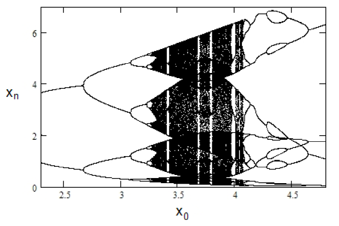
Figure 1: Bifurcations of solutions of Eq.(78) with a changing initial value; $a=4.6$ is fixed.

Stable solutions with periods 2, 4, 8, 12 and 16 can be easily identified in Figure 1. All of the solutions that appear in this figure represent coexisting stable orbits of Eq.(78). There are also periodic and non-periodic solutions which do not appear in Figure 1 because they are unstable (e.g., the fixed point $\bar{x}=2.3$). Additional bifurcations of both periodic and non-periodic solutions occur outside the range 2.3-4.8 which are not shown.

Understanding the global behaviors of solutions of Eq.(78) is relatively easy if we examine its SC factorization given by (76) and (77). Here $k=1$ and

$$\psi_{0}(t)=e^{-t},\quad\psi_{1}(t)=te^{-t},\quad\beta_{n}=e^{a}\text{ for all }n.$$

Thus (74) takes the form

$$\psi_{0}(t)^{c}\psi_{1}(t) =t^{c^{2}}\text{ for all }t>0$$

$$e^{-ct}te^{-t} =t^{c^{2}}\text{ for all }t>0$$

The last equality is true if $c=-1,$ which leads to the form symmetry

$$h_{1}(t)=t^{-1}\psi_{0}(t)^{-1}=\frac{1}{te^{-t}}\Rightarrow H(u_{0},u_{1})=\frac{u_{0}}{u_{1}e^{-u_{1}}}$$

and SC factorization

$$r_{n+1} =\frac{e^{a}}{r_{n}},\quad r_{0}=x_{0}h_{1}(x_{-1})=\frac{x_{0}}{x_{-1}e^{-x_{-1}}}$$ (79)

$$x_{n+1} =\frac{r_{n+1}}{h_{1}(x_{n})}=r_{n+1}x_{n}e^{-x_{n}}.$$ (80)

All positive solutions of (79) with $r_{0}\neq e^{a/2}$ are periodic with period 2:

$$\left\{r_{0},\frac{e^{a}}{r_{0}}\right\}=\left\{\frac{x_{0}}{x_{-1}e^{-x_{-1}}},\frac{x_{-1}e^{a-x_{-1}}}{x_{0}}\right\}.$$

Hence the orbit of each nontrivial solution $\{x_{n}\}$ of (78) in the plane is restricted to the pair of curves

$$\xi_{1}(t)=\frac{e^{a}}{r_{0}}te^{-t}\quad\text{and\quad}\xi_{2}(t)=r_{0}te^{-t}.$$ (81)

Now, if $x_{-1}$ is fixed and $x_{0}$ changes, then $r_{0}$ changes proportionately to $x_{0}$. These changes in initial values are reflected as changes in parameters in (80). The orbits of the one dimensional map $bte^{-t}$ where $b=r_{0}$ or $e^{a}/r_{0}$ exhibit a variety of behaviors as the parameter $b$ changes according to well-known rules such as the fundamental ordering of cycles and the occurrence of chaotic behavior with the appearance of period-3 orbits when $b$ is large enough. Eq.(80) splits the orbits evenly over the pair of curves (81) as the initial value $x_{0}$ changes and coexisting, qualitatively different stable solutions appear.

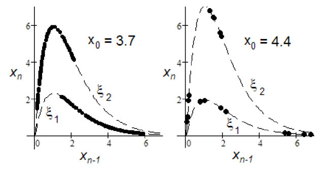
Figure 2: Two of the orbits in Figure 1 shown here on their loci of two curves $\xi_{1}$, $\xi_{2}$ in the state space.

Figure 2 shows the orbits of (78) for two different initial values $x_{0}$ with $a=4.6;$ the first 100 points of each orbit are discarded in these images so as to highlight the asymptotic behavior of each orbit.

5 Concluding remarks

In this article we covered the basic theory of reduction of order in higher order difference equations by semiconjugate factorization. Needless to say, a great deal more remains to be done in this area before a sufficient level of maturity is reached. It is necessary to generalize and extend various ideas discussed above. In addition, a more detailed theory is necessary for a full discussion of type-$(m,k)$ reductions for all $m$.

The list of things needing proper attention is clearly too long for a research article. An upcoming book [17] is devoted to the topic of semiconjugate factorizations and reduction of order. This book consolidates the existing literature on the subject and offers in-depth discussions, more examples, additional theory and lists of problems for further study.

References

• [1] Alseda, L. and Llibre, J., Periods for triangular maps, Bull. Austral. Math. Soc., 47 (1993) 41-53.
• [2] Bourgault, S. and Thomas, E.S., A note on the existence of invariants, J. Difference Eqs. and Appl., 7 (2001) 403-412.
• [3] Byrnes, G.B., Sahadevan, R., Quispel, G.R.W., Factorizable Lie symmetries and the linearization of difference equations, Nonlinearity, 8 (1995) 443-459.
• [4] Dehghan, M., Mazrooei-Sebdani, R. and Sedaghat, H., Global behavior of the Riccati difference equation of order two, J. Difference Eqs. and Appl., to appear.
• [5] Dehghan, M., Kent, C.M., Mazrooei-Sebdani, R., Ortiz, N.L. and Sedaghat, H., Monotone and oscillatory solutions of a rational difference equation containing quadratic terms, J. Difference Eqs. and Appl., 14 (2008) 1045-1058.
• [6] Dehghan, M., Kent, C.M., Mazrooei-Sebdani, R., Ortiz, N.L. and Sedaghat, H., Dynamics of rational difference equations containing quadratic terms, J. Difference Eqs. and Appl., 14 (2008) 191-208.
• [7] Elaydi, S.N., An Introduction to Difference Equations (2nd ed.) Springer, New York, 1999.
• [8] Franke, J.E., Hoag, J.T. and Ladas, G., Global attractivity and convergence to a two cycle in a difference equation, J. Difference Eqs. and Appl., 5 (1999) 203-209.
• [9] Grove, E.A., Kocic, V.L. and Ladas, G., Classification of invariants for certain difference equations, in Advances in Difference Equations, Proceedings of the second conference on difference equations and applications, Gordon and Breach, 1997, 289-294.
• [10] Hydon, P.E., Symmetries and first integrals of ordinary difference equations, Proc. R. Soc. Lond. A 456 (2000) 2835-2855.
• [11] Jordan, C., Calculus of Finite Differences, Chelsea, New York, 1965.
• [12] Kent, C.M. and Sedaghat, H., Convergence, periodicity and bifurcations for the two-parameter absolute difference equation, J. Difference Eqs. and Appl., 10 (2004) 817-841.
• [13] Levi, D., Trembley, S. and Winternitz, P., Lie point symmetries of difference equations and lattices, J. Phys. A: Math. Gen., 33 (2000) 8507-8523.
• [14] Maeda, S., The similarity method for difference equations, IMA J. Appl. Math., 38 (1987) 129-134.
• [15] Mortveit, H.S., Reidys, C.M., An Introduction to Sequential Dynamical Systems, Springer, New York, 2008.
• [16] Sahadevan, R., On invariants for difference equations and systems of difference equations, J. Math. Analy. Appl. 233 (1999) 498-507.
• [17] Sedaghat, H., Form Symmetries and Reduction of Order in Difference Equations (forthcoming) CRC Press, Boca Raton, 2010.
• [18] Sedaghat, H., Every homogeneous difference equation of degree one admits a reduction in order, J. Difference Eqs. and Appl., 15 (2009) 621-624.
• [19] Sedaghat, H., Reduction of order in difference equations by semiconjugate factorizations, Int. J. Pure and Appl. Math., 53 (2009) 377-384.
• [20] Sedaghat, H., Global behaviors of rational difference equations of orders two and three with quadratic terms, J. Difference Eqs. and Appl., 15 (2009) 215-224.
• [21] Sedaghat, H., Periodic and chaotic behavior in a class of second order difference equations, Adv. Stud. Pure Math., 53 (2009) 321-328.
• [22] Sedaghat, H., Order-Reducing Form Symmetries and Semiconjugate Factorizations of Difference Equations (2008) http://arxiv.org/abs/0804.3579
• [23] Sedaghat, H., Reduction of order of separable second order difference equations with form symmetries, Int. J. Pure and Appl. Math., 27 (2008) 155-163.
• [24] Sedaghat, H., Nonlinear Difference Equations: Theory with Applications to Social Science Models, Kluwer, Dordrecht, 2003.
• [25] Sedaghat, H., Semiconjugates of one-dimensional maps, J. Difference Eqs. and Appl., 8 (2002) 649-666.
• [26] Smital, J., Why it is important to understand the dynamics of triangular maps, J. Difference Eqs. and Appl., 14 (2008) 597-606.