$p$–wave pion production from nucleon-nucleon collisions

Abstract

We investigate $p$-wave pion production in nucleon-nucleon collisions up to next-to-next-to-leading order in chiral effective field theory. In particular, we show that it is possible to describe simultaneously the $p$-wave amplitudes in the $pn\to pp\pi^{-}$, $pp\to pn\pi^{+}$, $pp\to d\pi^{+}$ channels by adjusting a single low-energy constant accompanying the short-range operator which is available at this order. This study provides a non-trivial test of the applicability of chiral effective field theory to reactions of the type $NN\to NN\pi$.

I Introduction

With the advent of chiral perturbation theory (ChPT), the low-energy effective field theory (EFT) of QCD, high accuracy calculations for hadronic reactions with a controlled error estimation have become possible chpt1 ; chpt2 . In that framework, $\pi\pi$ pipi and $\pi N$ piN scattering observables and nuclear forces NN are calculated based on a perturbative expansion in $q/\Lambda_{\chi}$ with $q$ referring to either a generic momentum of external particles or the pion mass $m_{\pi}$, and $\Lambda_{\chi}\sim$ 1 GeV being the chiral symmetry breaking scale. An extension of this scheme to pion production in nucleon-nucleon ($NN$) collisions turned out to be considerably more difficult. A straightforward application of the power counting proposed by Weinberg Weinberg:1990rz ; Weinberg:1991um to the reactions $NN\to NN\pi$ NNpi ; NNpicharged failed badly (see also Ref. BKMnovel where it was pointed out that the naive power counting using the heavy baryon formalism is not applicable above the pion production threshold). Indeed, for neutral pion production in $pp$ collisions, the corrections due to the next-to-leading order (NLO) increased the discrepancy with the data and, moreover, the next-to-next-to-leading order (NNLO) contributions turned out to be even larger than the NLO terms NNpiloops . The origin of these difficulties was identified quite early by Cohen et al. bira1 , see also rocha , who stressed that the additional new scale, inherent in reactions of the type $NN\to NN\pi$, needs to be accounted for in the power counting. Since the two nucleons in the initial state need to have sufficiently high kinetic energy to produce the onshell pion in the final state, the initial center-of-mass momentum needs to be larger than

$$p_{\rm thr}=\sqrt{M_{N}\,m_{\pi}}\,,\quad\mbox{with}\quad\frac{p_{\rm thr}}{\Lambda_{\chi}}\simeq\ 0.4\,,$$ (1)

where $m_{\pi}$ and $M_{N}$ refer to the the pion and nucleon mass, respectively. The proper way to include this scale was presented in Ref. ch3body and implemented in Ref. withnorbert , see Ref. report for a review article. As a result, pion $p$-wave production is governed by the tree-level diagrams up to NNLO in the modified power counting scheme of Ref. ch3body . On the other hand, for pion $s$-wave production, pion loops start to contribute already at NLO. It was demonstrated in Ref. lensky2 that all irreducible loop contributions at NLO cancel altogether, and the net effect of going to NLO was shown to increase the most important operator for charged pion production, first investigated in Ref. koltunundreitan , by a factor of 4/3. This was sufficient to overcome the apparent discrepancy with the data in that channel. But the neutral pion channel is more challenging — it still calls for a calculation of subleading loop contributions. First steps in this direction were taken in Refs. subloops . We further emphasize that the $\Delta$(1232) isobar should be taken into account explicitly as a dynamical degree of freedom bira1 because the Delta-nucleon mass difference, $\Delta M$, is also of the order of $p_{thr}$. This general argument was confirmed numerically in phenomenological calculations jouni ; ourdelta ; ourpols .

Pion $p$-wave production in $NN$ collisions receives an important contribution from the leading $(\bar{N}N)^{2}\pi$ contact term in the effective Lagrangian, which also figures importantly in the three-nucleon force ch3body ; pdchiral . In addition, the same operator also contributes to the processes $\gamma d\to\pi NN$ gammad ; gammad_nn and $\pi d\to\gamma NN$ gardestig ; gardestig2 as well as to weak reactions such as, e.g., tritium beta decay and proton-proton $(pp)$ fusion park2 ; phillips , as visualized in Fig. 1.

Figure 1: Illustration of the various reactions, where the leading $(N\bar{N})^{2}\pi$-contact term contributes.

Notice that this operator appears in the above reactions in very different kinematics, ranging from very low energies for both incoming and outgoing $NN$ pairs in $pd$ scattering and the weak reactions up to relatively high initial energies for the $NN$ induced pion production. In Ref. gazit it was shown that both the ³H and ³He binding energies and the triton $\beta$-decay can be described with the same contact term. However, an apparent discrepancy between the strength of the contact term needed in $pp\to pn\pi^{+}$ and in $pp\to de^{+}\nu_{e}$ was reported in Ref. nakamura . If the latter observation were true, it would certainly question the applicability of chiral EFT to the reactions $NN\to NN\pi$.

To better understand the discrepancy reported in Ref. nakamura , in this paper we simultaneously analyze different pion production channels. In particular, we calculate the $p$-wave amplitudes for the reactions $pn\to pp\pi^{-}$, $pp\to pn\pi^{+}$, and $pp\to d\pi^{+}$. Note that even in these channels the contact term occurs in entirely different dynamical regimes. For the first channel $p$-wave pion production goes along with the slowly moving protons in the ${{}^{1}\!}S_{0}$ final state whereas for the other two channels the ${{}^{1}\!}S_{0}$ $pp$ state is to be evaluated at the relatively large initial momentum. Notwithstanding, all three channels of the reaction $NN\to NN\pi$ seem to give consistent results for the low-energy constant (LEC) $d$ that represents the strength of the contact term, as we will show in the present paper. We discuss which additional data are needed to further support this conclusion. We argue that the origin of the discrepancy reported in Ref. nakamura is not due to the different kinematics of $NN\to NN\pi$ and $pp$ fusion, but rather in the inconsistency in the partial wave amplitudes used in the analysis. In addition, we also comment on technical issues related to the work of Ref. nakamura .

Our manuscript is organized as follows: In Sec. II we discuss the general features and the relevant observables for $p$-wave pion production. In Sec. III the power counting is outlined with special emphasis on the $p$-wave amplitudes. Our results for the various pion production channels are presented in Sec. IV. Here, we also discuss the role of the leading $\pi N$ scattering parameters, $c_{3}$ and $c_{4}$, for the $p$-wave pion production amplitudes. We close with a short Summary.

II General Remarks

It is not obvious, a priori, that with just a single contact term, which contributes to the various reactions shown in Fig. 1, a consistent description of all these channels can be achieved. The purpose of the contact term is twofold: it should, on the one hand, absorb any sensitivities to the employed $NN$ wave functions and in this way remove the model dependence in the evaluation of the observables. On the other hand, it provides a parameterization of the short-range physics that contributes to the process being considered. Thus, the strength of the contact term is necessarily dependent on the method applied to regularize the integrals (typically a cut-off) and also on the $NN$ interaction that is used for generating the wave functions.

For the case at hand the contact term connects $NN$ $S$-waves in the initial state with $NN$ $S$-waves in the final state. Since the contact term is a local four-nucleon operator, after including the NN distortions its contribution scales as the product of the initial and final NN wave functions at the origin. Each of these wave functions, in turn, may be represented by the inverse of the corresponding Jost function goldbergerwatson . The reason why it is expected to be possible that the same contact term can be used in all reactions listed above is that the energy dependence of the Jost function is fixed by the onshell $NN$ data and is therefore independent of the unknown short range physics. Specifically, the $NN$ distortions can be represented as an integral over the relevant phase shifts by means of the so-called Omnès function Omnes — see also the discussion in Ref. Ashot . This is correct up to contributions from the left-hand cuts and the high energy behaviour of the $NN$ interaction, both are expected to be of higher order in the expansion. As opposed to the energy dependence, the overall scale of the distortions can be shown to be sensitive to things like the $NN$ interaction and the cut-off employed withkanzo . Clearly, what needs to be assumed in the argument given is that there is a proper separation of scales in the problem. Note that the expansion parameter $p_{\rm thr}/\Lambda_{\chi}\sim 0.4$ is quite large. In this sense a consistent description of all mentioned reactions with the same contact term provides a non-trivial test of the applicability of the chiral expansion to pion production in $NN$ collisions.

One might ask why we take the effort of this study, since in Ref. nakamura it was already shown that a consistent description is not possible. The answer is twofold: first of all, we found that the partial wave decomposition of Ref. Flammang , the result of which was used in Ref. nakamura , is not correct (see discussion in Sec.IV.3) — this is why we decided to directly compare to the data in the present work. Secondly, there is also a conceptual problem in the work of Ref. nakamura : as was outlined above, as long as different phase-equivalent $NN$ interactions are used, it should be possible to absorb the model dependence of the calculation in a single counter term up to higher-order corrections. However, in Ref. nakamura pion production from initial $NN$ and $N\Delta$ states is not treated on equal footing. Rather the contribution from the $\Delta$ isobar excitation is added on top of and independently of the employed $NN$ interactions. Thus, it is quite possible that the utilized $NN\to N\Delta$ transition potential is too strong. Specifically, it is not constrained by the empirical $NN$ phase shifts as it is the case when considering the $NN$ and $N\Delta$ amplitudes consistently within a coupled-channel (Lippmann-Schwinger-like) scattering equation jouni . In this sense, it should not come as a surprise that it was not possible to absorb the model dependencies in a single counter term within the scheme used in Ref. nakamura . To avoid this problem, in this work we employ the coupled-channel $NN$ model of Ref. CCF which involves the $NN\to N\Delta$ transition potential.

Eventually all reactions shown in Fig. 1 should be analysed consistently. This would, however, require a calculation to third order in the chiral expansion of the process $\gamma d\to\pi NN$ and $\pi d\to\gamma NN$ or a rather involved three-nucleon calculation for the tritium beta decay which goes beyond the scope of this work. Instead, as a next step in this ambitious program, we analyse here in detail various pion production channels. Notice that although these reactions appear to have similar kinematics, the relevant transition for the reaction $pn\to pp\pi^{-}$ involves very low momenta in the $NN$ ${}^{1\!}S_{0}$ state and considerably higher momenta ($\sim p_{\rm thr}$) in the ${}^{3\!}S_{1}$ channel while the situation is just opposite for the reactions $pp\to(d/pn)\pi^{+}$. Thus, a simultaneous description of these reaction with a single short-range operator indeed provides a highly nontrivial consistency test of our approach. Notice further that the $(N\bar{N})^{2}\pi$ short-range operator we are interested in here does not contribute to the $pp\to pp\pi^{0}$ transition which is, therefore, not considered in the present work. Thus, the only reactions of interest for this study are $pp\to(pn/d)\pi^{+}$ and $pn\to pp\pi^{-}$. Here the relevant transitions are ${{}^{1\!}}S_{0}\to{{}^{3\!}}S_{1}p$ for the former and $({{}^{3\!}}S_{1}-{{}^{3\!}}D_{1})\to{{}^{1\!}}S_{0}p$ for the latter, where the small letter labels the pion angular momentum. Since the main focus of this work is on the role of the contact term, we will concentrate on observables where the final $NN$ system is in an $S$-wave — which largely simplifies the numerical work. However, as outlined below, the contribution of $NN$ $P$-waves to observables might be relevant for the reaction $pp\to pn\pi^{+}$. This potential problem renders this channel not very convenient for the extraction of the counter term, as will be discussed in Sec. IV.

To be specific, we calculate in this work the differential cross sections and analyzing powers for the reactions $pp\to d\pi^{+}$, $pp\to pn\pi^{+}$, and $pn\to(pp)_{{}^{1\!}S_{0}}\pi^{-}$. Here the symbol $(pp)_{{}^{1\!}S_{0}}$ indicates that in the corresponding measurement the final $pp$ relative momentum was restricted kinematically to be less than 38 MeV/c ($M_{pp}-2M_{N}\leq 1.5$ MeV) which leads to a projection on the ${{}^{1\!}}S_{0}$ $pp$ final state. For all the mentioned observables experimental data are available or will be available soon in the energy range of relevance here. Besides the anisotropy of the pion angular distributions, all observables are sensitive to both $s$- and $p$-wave pion production. Although there exists an NLO calculation for $s$-wave pion production in $pp\to d\pi^{+}$ using ChPT, its theoretical uncertainty is still sizable lensky2 . For $s$-wave pion production accompanied by a transition of an isospin-one $NN$ pair to an isospin-one $NN$ pair (e.g. in $pp\to pp\pi^{0}$), no sufficiently accurate ChPT calculation is available at present. Since we focus here on the $p$-wave amplitudes, we extract the $s$-wave amplitudes directly from the data in order to minimize the uncertainties of our calculation. The phase of these amplitudes is then imposed using the Watson theorem goldbergerwatson , see the discussion in Sec. IV.

It is well known that $p$-wave pion production in $pp\to d\pi^{+}$ and in $pp\to pn\pi^{+}$ is strongly dominated by the transition ${{}^{1\!}}D_{2}\to{{}^{3\!}}S_{1}p$ due to a strong coupling of the initial $NN$ state to the ${{}^{5\!}}S_{2}$ $N\Delta$ state ericsonweise . Therefore, the amplitude we are interested in has only a minor impact on the observables. In other words, the uncertainty for the extraction of the counter term from these reactions will be significant. The situation is much more promising for the reaction $pn\to pp\pi^{-}$: here the amplitude of interest is the leading $p$-wave. In addition, the strength of the $s$-wave amplitude can be taken from the reaction $pp\to pp\pi^{0}$ using isospin symmetry and correcting for the final state interaction (FSI) as discussed in Sec. IV.4. Unfortunately, no data are presently available for $pn\to pp\pi^{-}$ at sufficiently low energies. Nevertheless, as will be shown below, already the higher-energy data provide some insights. In addition, data at lower excess energies will be available soon ANKE .

The goal of the present investigation is to explore whether it is possible to obtain a simultaneous description of all $NN\to NN\pi$ channels. A more quantitative study including a statistical analysis of the data and an estimation of the theoretical uncertainty is postponed until accurate experimental data will become available for $pn\to pp\pi^{-}$ at low energies.

III Formalism

Our calculations are based on the effective chiral Lagrangian with explicit $\Delta$ degrees of freedom. The leading $\pi N$ and $\pi N\Delta$ interaction terms read OvK ; ulfbible

$${\cal L}^{(0)}=N^{\dagger}\left[\frac{1}{4f_{\pi}^{2}}\mbox{\boldmath$\tau$}\cdot(\dot{\mbox{\boldmath$\pi$}}\times{\mbox{\boldmath$\pi$}})+\frac{g_{A}}{2f_{\pi}}\mbox{\boldmath$\tau$}\cdot\vec{\sigma}\cdot\vec{\nabla}\mbox{\boldmath$\pi$}\right]N+\frac{h_{A}}{2f_{\pi}}\left[N^{\dagger}(\mbox{\boldmath$T$}\cdot\vec{S}\cdot\vec{\nabla}\mbox{\boldmath$\pi$})\Psi_{\Delta}+h.c.\right]+\cdots\ ,$$

while the first corrections have the form

$${\cal L}^{(1)} = \frac{1}{8M_{N}f_{\pi}^{2}}(iN^{\dagger}\mbox{\boldmath$\tau$}\cdot(\mbox{\boldmath$\pi$}\times\vec{\nabla}\mbox{\boldmath$\pi$})\cdot\vec{\nabla}N+h.c.)-\frac{1}{f_{\pi}^{2}}N^{\dagger}\bigg{[}c_{3}(\vec{\nabla}\mbox{\boldmath$\pi$})^{2}+\frac{1}{2}\left(c_{4}+\frac{1}{4M_{N}}\right)$$ (2)

$$\times \varepsilon_{ijk}\varepsilon_{abc}\sigma_{k}\tau_{c}\partial_{i}\pi_{a}\partial_{j}\pi_{b}\bigg{]}N-\frac{d}{f_{\pi}}N^{\dagger}(\mbox{\boldmath$\tau$}\cdot\vec{\sigma}\cdot\vec{\nabla}\mbox{\boldmath$\pi$})N\,N^{\dagger}N+\cdots\,\ .$$

The ellipses stand for further terms which are not relevant for the present study. In the equations above $f_{\pi}$ denotes the pion decay constant in the chiral limit, $g_{A}$ is the axial-vector coupling of the nucleon, $h_{A}$ is the $\Delta N\pi$ coupling, $N$ and $\Psi_{\Delta}$ correspond to the nucleon and Delta fields, respectively, and $\vec{S}$ and $T$ are the transition spin and isospin matrices, normalized according to:

$$S_{i}S_{j}^{\dagger}=\frac{1}{3}(2\delta_{ij}-i\epsilon_{ijk}\sigma_{k})\ ,\quad\quad T_{i}T_{j}^{\dagger}=\frac{1}{3}(2\delta_{ij}-i\epsilon_{ijk}\tau_{k})\ .$$ (3)

We also emphasize that the effective Lagrangian of Ref. OvK contains another $(\bar{N}N)^{2}\pi$ contact operator which can be shown to be redundant as a consequence of the Pauli principle ch3body ; pdchiral ; park2 .

We are now in the position to discuss the relevant scales and counting rules for $p$-wave pion production. We assign the outgoing two-nucleon relative momentum $p^{\prime}$ and the outgoing pion momentum $k_{\pi}$ to be of order of $m_{\pi}$ and introduce the expansion parameter

$$\chi\simeq\frac{k_{\pi}}{p}\simeq\frac{p^{\prime}}{p}\simeq\frac{m_{\pi}}{p}\simeq\frac{p}{M_{N}}\simeq\frac{\Delta M}{M_{N}}$$ (4)

where $p\simeq p_{\rm thr}$ is the initial two-nucleon relative momentum. The counting rules for the time-dependent vertices, such as e.g. the Weinberg-Tomosawa (WT) vertex in ${\cal L}^{(0)}$, are discussed in detail in Refs. lensky2 ; NNpiMENU . At leading order one finds that the WT vertex is $\propto 2\omega_{\pi}$ with $\omega_{\pi}$ being the energy of the outgoing (onshell) pion. The diagrams contributing to the production operator at LO and at NLO are shown in Fig. 2 whereas the corresponding graphs at NNLO are depicted in Fig. 3.

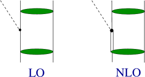
Figure 2: ”(Color online)” Leading and next-to-leading diagrams for the $p$-wave amplitudes of $NN\to NN\pi$. Single (double) solid lines denote nucleons (Deltas), dashed lines denote pions, green ellipses correspond to the $NN$ wave functions in the initial and final states.

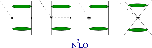
Figure 3: ”(Color online)” Diagrams that contribute at NNLO to the $p$-wave amplitudes of $NN\to NN\pi$. Subleading vertices are marked as $\odot$.

At NLO there are only diagrams in which the pion is produced through the excitation of the $\Delta$ resonance. The relative suppression of these diagrams as compared to the ones involving the nucleon is accounted for by the $\Delta$ propagator which is suppressed by $1/p$ as compared to $1/m_{\pi}$ in the nucleon case. To see that the diagrams in Fig. 3 indeed contribute at NNLO for $p$-wave pion production consider, as an example, the first graph in this figure. Its contribution can be estimated using dimensional analysis as follows:

$$\frac{\omega_{\pi}}{f_{\pi}^{2}}\frac{1}{p^{2}}\frac{k_{\pi}}{f_{\pi}}\simeq\frac{1}{f_{\pi}^{3}}\frac{k_{\pi}}{m_{\pi}}\frac{m_{\pi}}{M_{N}}.$$ (5)

Here we used that the outgoing pion momentum $k_{\pi}$ enters the $\pi NN$ vertex to allow for the $p$-wave amplitude. To understand the suppression factor this operator should be compared with the LO contribution ${k_{\pi}}/({f_{\pi}^{3}}{m_{\pi}})$. Thus, one gets an order $\chi^{2}$ suppression for the first diagram of Fig. 3. Similarly, using the $\pi\pi NN$ vertex from ${\cal L}^{(1)}$ in combination with the $p/f_{\pi}$-scaling for the $\pi NN$ vertex one arrives again at a $\chi^{2}$ suppression for the second diagram in Fig. 3. Further details can be found in Appendix A which contains explicit expressions for the diagrams shown in Figs. 2 and 3. Once the amplitudes are evaluated they need to be convoluted with proper $NN$ wave functions. Ideally, one would use wave functions derived from the same formalism, namely ChPT. However, up to now these are only available for energies below the pion production threshold NN . We therefore use the so-called hybrid approach, first introduced by Weinberg Weinberg:1991um , based on the transition operators derived within the effective field theory and convoluted with realistic wave functions CCF . This procedure should also provide reasonable results, however, a reliable uncertainty estimate is possible only at the level of the transition operator.

IV Results and Discussion

IV.1 Parameters of the calculation

To the order we are working, the following low-energy constants (LECs) appear in the calculation: $f_{\pi}$, $g_{A}$, $h_{A}$, $c_{3}$, $c_{4}$ and $d$. Only the last LEC cannot be taken from other sources, for its value strongly depends on the $NN$ wave functions employed. We adopt the following values of the parameters: $f_{\pi}=92.4$ MeV, $g_{A}=1.32$, $h_{A}\simeq 2.1g_{A}=2.77$, $c_{3}=-0.79$ GeV^-1 and $c_{4}=1.33$ GeV^-1. The values of the LECs $c_{3}$ and $c_{4}$ are taken from Ref. Evgeny . From the fit to $\pi N$ threshold parameters, two solutions for the $c_{i}$ are given in Ref. Evgeny corresponding to the different choices of $h_{A}$ ($h_{A}\simeq 2.1g_{A}$ and $h_{A}\simeq 2.1$). The sensitivity of the results to the different values of $c_{3}$ and $c_{4}$ will be also discussed. As already mentioned in the Introduction, the power counting scheme calls for a dynamical treatment of the $\Delta$ isobar as a result of the comparable numerical value of the Delta-nucleon mass difference and $p_{\rm thr}$. The implications of integrating out the $\Delta$ degrees of freedom for the processes at hand are discussed in Appendix B.

The deuteron wave function and the $NN$ scattering amplitudes used in the calculation are generated from the CCF $NN$ potential CCF . As described above, we do not calculate the $s$-wave pion amplitudes in this work but rather take both their strength and the phases directly from experiment. To be specific, for the reaction $pn\to pp\pi^{-}$ we aim at the description of the double differential cross sections and the analyzing power measured at TRIUMF hahn ; duncan and PSI Daum . Following the Watson theorem to parameterize the relevant ${{}^{3\!}}P_{0}\to{{}^{1\!}}S_{0}s$ amplitude, we use the ansatz $\tilde{C}e^{i\delta_{{}^{3\!}P_{0}}}\Psi^{(+)}_{p^{\prime}}(r=0)$, where the inverse Jost function in the ${{}^{1\!}}S_{0}$ partial wave, $\Psi^{(+)}_{p^{\prime}}(r=0)$, and the initial phase shift $\delta_{{}^{3\!}P_{0}}$ are calculated from the $NN$ model used, and the parameter $\tilde{C}$ is fitted to reproduce the corresponding amplitude extracted from the TRIUMF data using a partial wave analysis duncan ; duncan2 . It is interesting to note that the ${{}^{3\!}}P_{0}\to{{}^{1\!}}S_{0}s$ amplitude from the TRIUMF analysis at $\eta$=0.66 ($T_{lab}=353$ MeV) is about 25% larger than that extracted from the $pp\to pp\pi^{0}$ measurement at CELSIUS bilger . A similar inconsistency is discussed in Ref. cosytof where it is argued that the total cross sections at low energies for $pp\to pp\pi^{0}$ recently measured at COSY are about 50% larger than those at CELSIUS and IUCF as a result of the missing acceptance at small angles for both CELSIUS and IUCF.

For the reaction $pp\to d\pi^{+}$ the $s$-wave amplitude occurs in the ${{}^{3\!}}P_{1}\to{{}^{3\!}}S_{1}s$ partial wave and can be related to the total cross section at threshold. The most precise way of getting this quantity is to extract it from the width of pionic deuterium atom, measured at PSI with high accuracy Hauser ; Strauch . This procedure gives the following value of $\alpha$, the total cross section divided by $\eta$: $\alpha=252^{+5}_{-11}\ \mu$b pidexp . Thus, we adjust the magnitude of the ${{}^{3\!}}P_{1}\to{{}^{3\!}}S_{1}s$ amplitude to be in agreement with this observable.

As mentioned above the value of $d$ depends on the $NN$ interaction employed and on the method used to regularize the overlap integrals. Indeed, in Refs. park2 ; ch3body a strong sensitivity of the LEC $d$ to the regulator is reported. It therefore does not make much sense to compare values for $d$ as found in different calculations. What makes sense, however, is to compare results on the level of observables and this is what we will do below. We will adjust the value of $d$ in such a way to get the best simultaneous qualitative description of all channels of $NN\pi$.

IV.2 Reaction $pp\to d\pi^{+}$

We begin with a discussion of the results for the reaction $pp\to d\pi^{+}$. In Fig. 4,

\psfrag{A2/A0}{\large$\rm A_{2}/A_{0}$}\includegraphics[scale={0.3}]{Fig4a.eps}

\psfrag{A2/A0}{\large$\rm A_{2}/A_{0}$}\psfrag{Ay (90)}{\large$\rm A_{y}(90^{0})$}\includegraphics[scale={0.3},clip={}]{Fig4b.eps}

Figure 4: ”(Color online)” Results for $A_{2}/A_{0}$ (see Eq. 6) (left panel) and the analyzing power at 90 degrees (right panel) for the reaction $pp\to d\pi^{+}$ for different values for the strength of $d$ (in units $1/(f^{2}_{\pi}M_{N})$). Shown are $d=3$ (red solid line), $d=0$ (black dashed line), and $d=-3$ (blue dot-dashed line). The data are from Refs. Ritchie ; Heimberg ; Drochner ; Korkmaz ; Mathie . The strength and phase of the $s$-wave amplitude is fixed from data.

we compare our calculation for various values of $d$ with the experimentally available angular asymmetry parameter $A_{2}/A_{0}$. The coefficients $A_{i}$ are related to the unpolarized differential cross section via

$$\frac{d\sigma}{d\Omega}=A_{0}+A_{2}P_{2}(\cos\theta_{\pi})\ ,$$ (6)

with $P_{2}(x)$ being the second Legendre polynomial and $\theta_{\pi}$ the pion angle in the c.m. frame. We also show results for the analyzing power at 90 degrees. In both cases the observables are plotted as functions of the parameter $\eta$. Here and in what follows, the value of the LEC $d$ is always given in units $1/(f^{2}_{\pi}M_{N})$. Notice that at low energies, it is sufficient to just show the analyzing power at 90 degrees since its angular dependence is proportional to $\sin\theta_{\pi}$. To illustrate this we also present in Fig. 5 the analyzing power

\psfrag{Ay}{\large$\rm A_{y}$}\includegraphics[scale={0.52},clip={}]{Fig5.eps}

Figure 5: ”(Color online)” Results for the analyzing power at $\eta$=0.14 (upper panel) and $\eta$=0.21 (lower panel) as functions of the angle $\theta_{\pi}$ for the reaction $pp\to d\pi^{+}$ for different values of $d$. Shown are $d=3$ (red solid line), $d=0$ (black dashed line), and $d=-3$ (blue dot-dashed line). The data are from Ref. Korkmaz . The strength and phase of the $s$-wave amplitude is fixed from data.

as a function of the scattering angle for two different energies $\eta$=0.14 and $\eta$=0.21. At $\eta\simeq 0.5$ the angular dependence of the analyzing power starts to deviate significantly from $\sin\theta_{\pi}$ due to the onset of $d$-waves. Clearly, at these (and higher) energies we cannot expect our calculation to agree with the data anymore. As can be seen from the figures, the data at small $\eta$, especially the analyzing power, prefers a positive value for $d$ — our fit resulted in $d=3$ for the best value. To demonstrate the effect of the LEC $d$ on the observables, in Fig. 5 and in subsequent figures we also give the results with $d=0$ and with the negative LEC $d=$-3.

IV.3 Reaction $pn\to pp\pi^{-}$

We now turn to the reaction $pn\to pp\pi^{-}$. As it was already explained in Sec. II, for this reaction channel the relevant pion $p$-wave occurs in conjunction with the two-nucleon pair in the ${{}^{1\!}}S_{0}$ state. It is known experimentally that in the isospin-one channel the final $P$-wave diproton contributions ($Pp$ and $Ps$) start growing with the energy rather rapidly so that already for excess energies around 30 MeV they provide about 50% of the total cross section bilger . Therefore, in order to be sensitive to our particular amplitude one needs to isolate experimentally the $S$-wave diproton state by putting kinematical cuts on the two-nucleon relative momentum. This is exactly what was done in the experimental study of $pn\to pp\pi^{-}$ at TRIUMF hahn ; duncan . In particular, they measured the differential cross section $d^{2}\sigma/(d\Omega dm_{pp}^{2})$ and analyzing power $A_{y}$ for $T_{lab}=353$ MeV ($\eta$=0.66), where the final diproton relative momentum $p^{\prime}$ was restricted to be not larger than $38$ MeV/c ($M_{pp}-2M_{N}\simeq 1.5$ MeV). A similar measurement for the analyzing power was also performed at PSI Daum for $T_{lab}=345$ MeV and $pp$ invariant masses $M_{pp}-2M_{N}<6$ MeV. It is interesting to note that the positions of the peaks in $A_{y}$ seem to be somewhat different in these experiments (see Fig. 6), although the data of Ref. Daum have much larger uncertainties than those of Ref. hahn . Unfortunately, presently data for $pn\to pp\pi^{-}$ are only available at such high energies where our corresponding results in the $pp\to d\pi^{+}$ channel already start to deviate considerably from the experiment. Therefore, for the reaction $pn\to pp\pi^{-}$ we expect likewise only a qualitative description. Nevertheless, a comparison with the experimental data in this channel is quite instructive too and shows also a preference for a positive value of $d$ as visualized in Fig. 6. Fortunately, there will soon be a measurement for the same observables at lower energies at COSY ANKE . Once this data will be available we should be able to draw more quantitative conclusions on the value of the parameter $d$ needed for the reaction $pn\to pp\pi^{-}$.

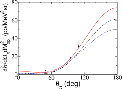
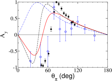
Figure 6: ”(Color online)” Results for $d^{2}\sigma/d\Omega_{\pi}dM^{2}_{pp}$ (left panel) and $A_{y}$ (right panel) for $pn\to pp(^{1}S_{0})\pi^{-}$. Shown are the results for $d=3$ (red solid line), $d=0$ (black dashed line) and $d=-3$ (blue dot-dashed line). The data is from TRIUMF hahn ; duncan (black squares) and from PSI Daum (blue circles) .

IV.4 Reaction $pp\to pn\pi^{+}$

The reaction $pp\to pn\pi^{+}$ is the most difficult and the least convenient one for the extraction of the contact term. Besides the fact that here, as in $pp\to d\pi^{+}$, pion $p$-wave production is mainly driven by the ${{}^{1\!}}D_{2}$ initial state, in addition $NN$ $P$-waves contribute for isospin-one as well as for isospin-zero $NN$ final states. At the energies considered in the experimental investigation, $\eta=$0.22, 0.42, and 0.5, the $Pp$ amplitudes may contribute significantly bilger ; complete ; pwpi0 . They should be particularly important in view of the smallness of the ${{}^{1\!}}S_{0}$ amplitude — even small contributions to $A_{2}$, see Eqs. (6) and (8), can affect the partial wave analysis considerably. In the partial wave analysis performed in Ref. Flammang , these $Pp$ contributions were not taken into account at all. Also there are contributions to $A_{0}$ from the isospin-one $NN$ final states that potentially increase the uncertainty of the analysis, especially in view of the differences in the experimental results in $pp\to pp\pi^{0}$ as already discussed above. These arguments alone cast serious concerns on the partial wave analysis performed in Ref. Flammang . But there is an even more direct evidence of problems with the extraction of the partial wave amplitudes of Ref. Flammang which we now discuss in detail. The observables measured for the reaction ${\vec{p}}p\to pn\pi^{+}$ in Ref. Flammang include the coefficients $A_{0}$ and $A_{2}$ in the differential cross section, see Eq. (6) and the analyzing power $Ay(90^{\circ})$. Neglecting the $Pp$ contributions these observables can be expressed in terms of the three partial wave amplitudes with the isospin-zero $pn$-state $a_{0}$ (${{}^{1\!}}S_{0}\to{{}^{3\!}}S_{1}p$) (the single amplitude, where the $(N\bar{N})^{2}\pi$ contact term contributes), $a_{1}$ (${{}^{3\!}}P_{1}\to{{}^{3\!}}S_{1}s$), $a_{2}$ (${{}^{1\!}}D_{2}\to{{}^{3\!}}S_{1}p$) and the contribution of the isospin-one channel denoted as $A_{0}^{I=1}$ via

$$A_{0} = \frac{|a_{0}|^{2}+|a_{1}|^{2}+|a_{2}|^{2}}{4}+A_{0}^{I=1},$$ (7)

$$A_{2} = \frac{|a_{2}|^{2}}{4}-\frac{1}{\sqrt{2}}{\rm Re}[a_{0}a_{2}^{*}],$$ (8)

$$A_{y}(90^{\circ})\left(A_{0}-\frac{A_{2}}{2}\right) = \frac{1}{4}(\sqrt{2}{\rm Im}[a_{1}a_{0}^{*}]+{\rm Im}[a_{1}a_{2}^{*}]),$$ (9)

where $(A_{0}-{A_{2}}/{2})$ is just ${d\sigma}/{d\Omega}(90^{\circ})$ from Eq. (6). Using the system of Eqs. (7)-(9) one can determine the amplitudes $a_{0},\ a_{1}$ and $a_{2}$ provided one knows the isospin-one piece $A_{0}^{I=1}$. The latter was extracted in Ref. Flammang from the measurement of the total cross section in the reaction $pp\to pp\pi^{0}$ reported in Ref. Meyer . However, the FSI in the $pp\to pp\pi^{0}$ reaction is very different to that in the $pp\to pn\pi^{+}$ channel. To estimate the difference note that in the energy region studied, which is less than $20$ MeV, the dominant partial wave is the one where the final two-nucleon state is in the $S$-wave. In this case the correction factor would be proportional to the ratio of the inverse Jost functions squared integrated over the phase space

$$R=\frac{\int d^{3}p^{\prime}k_{\pi}|F_{\mathrm{pn}}(p^{\prime})|^{2}}{\int d^{3}p^{\prime}k_{\pi}|F_{\mathrm{pp}}^{\rm CC}(p^{\prime})|^{2}}\ ,$$ (10)

where $F_{\mathrm{pn}}(p^{\prime})$ and $F_{\mathrm{pp}}^{\rm CC}(p^{\prime})$ are the inverse Jost functions for the $pn$ and $pp$ ${{}^{1\!}}S_{0}$ states, respectively. As discussed above, although the Jost function itself depends on the $NN$ model used, its energy dependence does not. We may, therefore, evaluate $R$ using any sensible model for the $NN$ interaction. For a separable $NN$ potential there exists an analytic expression for the Jost function in the $pp$ system in the presence of the Coulomb interaction vanher ; KDT . Using it one finds that the ratio $R$ is about 1.5 for $\eta=0.22$ and about 1.2 for $\eta=0.42$. Similar results are obtained using the CCF $NN$ interaction CCF . Thus, compared to the original analysis performed in Ref. Flammang , the isospin-one contribution at $\eta=0.22$ should be enhanced by more than a factor of two if, in addition, one utilizes the new, larger experimental data from COSY for the total cross section for $pp\to pp\pi^{0}$ cosytof . This change, of course, will significantly affect the results of the partial wave analysis. Given the above difficulties with the partial wave analysis of Ref. Flammang , we decided to compare our results directly to the experimentally measured quantities. Aiming presently at a qualitative description of the data, we will not include the $Pp$-states in this work.

The results of our calculation for $A_{2}$ are shown in Fig. 7. Again,

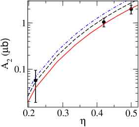
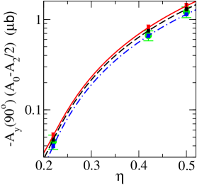
Figure 7: ”(Color online)” Results for the magnitude of $A_{2}$ (left panel) and $A_{y}(90^{\circ})(A_{0}-A_{2}/2)$ (right panel) for the reaction $pp\to pn\pi^{+}$ for different values of the contact term. The notation of curves is the same as in Fig. 4. The data are from Ref. Flammang .

positive values of the contact term with $d\sim 3$ seem to be preferred. We emphasize, however, that these results should be treated with care since the calculations at higher energies can be affected by $P$-wave contributions whereas the lowest point is not very sensitive to the value of $d$ due to the large experimental uncertainty. We can also check whether our results are consistent with the measurement of the analyzing power that is related to our amplitudes via Eq. (9). To allow for this comparison, however, we need to know the pion $s$-wave amplitude $a_{1}$. At present, this quantity is known theoretically only up-to-and-including terms at NLO. Therefore, to minimize the uncertainty of the current study, we extract this amplitude directly from data on the total cross section in $pp\to pn\pi^{+}$ through Eq. (7). We employ the amplitude $A_{0}^{I=1}$ consistent with the data at COSY and correct for the FSI factor as described above and take the amplitudes $a_{0}$ and $a_{2}$ from our NNLO calculation. In the right panel of Fig. 7 we compare our results for $A_{y}(90^{\circ})\left(A_{0}-{A_{2}}/{2}\right)$ with the corresponding data. Since we use the experimental total cross sections to extract $a_{1}$, our results, given by red ($d=3$), black ($d=0$) and blue ($d=-3$) squares in the right panel of Fig. 7, can be presented at specific energies only. The squares include the experimental uncertainty in the total cross section $A_{0}$ used to extract $a_{1}$. To guide the eye, we also show the results of interpolations between the three energies. It is seen that the magnitude $A_{y}(90^{\circ})\left(A_{0}-{A_{2}}/{2}\right)$ is much less sensitive to the value of the LEC $d$ than, e.g., $A_{2}$. Notice further that the experimental points do not include a 12% uncertainty due to systematic errors in $A_{0}$ and $A_{2}$.

Since we do not know the contribution of the $NN$ $P$-waves to the $pp\to pn\pi^{+}$ observables at present, and an improved partial wave analysis would require a careful study of various uncertainties, we do not try to extract $a_{0}$ from the data. However, in order to illustrate the potential effect of the changes discussed above (up to $NN$ $P$-waves) on $a_{0}$, in Fig. 8 we show the results of our calculation for $a_{0}$ in comparison to the old extraction of Ref. Flammang . Evidently, although all data presented in Ref. Flammang are in a good agreement with our calculation (as demonstrated in Fig. 7), the partial wave amplitude is not at all described — see solid curve for our results with $d$=3 in Fig. 8, which illustrates clearly that the partial wave solution given in Ref. Flammang should be abandoned. It is interesting to note that in Ref. nakamura it was stressed that a positive value for $a_{0}$ is necessary in order to achieve a result for pion production that is consistent with the ones for the weak rates. This is in accord with our findings based solely on the data for $NN\to NN\pi$. Here we do not aim at a more quantitative comparison with Ref. nakamura , because of the technicalities discussed in the beginning of Sec. II.

\psfrag{a0}{\Large$\rm\ a_{0}\ (\,{{\mu b}^{1/2}}\,)$}\includegraphics[scale={0.52},clip={}]{Fig8.eps}

Figure 8: ”(Color online)” Comparison of $a_{0}$ as it results from our analysis in comparison to the partial wave amplitude extracted in Ref. Flammang . The notation of curves is the same as in Fig. 4. Since our calculations well describe all observables of Ref. Flammang , this figure nicely illustrates the problem of the partial wave decomposition of this reference.

Finally, we would like to discuss the sensitivity of our results to the parameters $c_{i}$. As shown in Appendix A, for the ${{}^{1\!}}S_{0}\to{{}^{3\!}}S_{1}$ or ${{}^{3\!}}S_{1}\to{{}^{1\!}}S_{0}$ $NN$ transitions the parameters $c_{i}$ occur in the combination $C_{i}^{{}^{3\!}S_{1}}=c_{3}/2+c_{4}+1/(4M_{N})$. This combination appears to be largely constrained by the $\pi N$ data since the different sets of $c_{i}$ from the recent analysis Evgeny give basically the same value for $C_{i}^{{}^{3\!}S_{1}}$. In addition, to the order we are working at, this combination is fully absorbed in the counter term since the corresponding potential for $NN\to NN\pi$, see the second diagram in Fig. 3, is just a constant up to higher order terms

$$V^{c_{i}}_{{}^{1\!}S_{0},^{3\!}S_{1}}\sim C_{i}^{{}^{3\!}S_{1}}\frac{(\vec{p}-\vec{p}\,^{\prime})^{2}}{(\vec{p}-\vec{p}\,^{\prime})^{2}+m_{\pi}^{2}}=C_{i}^{{}^{3\!}S_{1}}\left(1+{\mathcal{O}}(\chi^{2})\right).$$ (11)

Due to a coupled channel effect, the same combination of $c_{i}$ also contributes in the ${{}^{3\!}}D_{1}\to{{}^{3\!}}S_{1}\to{{}^{1\!}}S_{0}p$ partial wave. The situation is different when $D$-waves contribute at the level of the transition operator. The combinations of $c_{i}$ in the ${{}^{3\!}}D_{1}\to{{}^{1\!}}S_{0}p$ amplitude for $pn\to pp\pi^{-}$ and in the ${{}^{1\!}}D_{2}\to{{}^{3\!}}S_{1}p$ amplitude for $pp\to(d/pn)\pi^{+}$ will influence the observables, for at the order we are working at there is no contact term that can absorb the resulting dependence on the LECs $c_{i}$. It is worth mentioning that the combinations of $c_{i}$ in these partial waves are constrained only weakly by $\pi N$ data. In particular, the combination of $c_{i}$ in the ${{}^{3\!}}D_{1}$ partial wave, $C_{i}^{{}^{3\!}D_{1}}=c_{3}-c_{4}-1/(4M_{N})$, changes from 2 to 7 depending on which of the sets of $c_{i}$ given in Ref. Evgeny is used. Thus, we conclude that the reaction $NN\to NN\pi$ may serve as an additional source of information to constrain the $c_{i}$’s, complementary to the $\pi N$ Evgeny ; bernardLEC and $NN$ timmermans data (see, however, Ref. entem for some criticism). However, for a more quantitative study of the constraints implied by pion production, and by $\pi N$- and $NN$ scattering data, a more complete and consistent analysis is necessary, which we postpone to a future work.

V Summary and Outlook

We performed a calculation of $p$-wave pion production amplitudes in $NN$ collisions in three different channels ($pn\to pp\pi^{-}$, $pp\to d\pi^{+}$ and $pp\to pn\pi^{+}$) in the framework of chiral effective field theory. The relevant partial wave transition that depends on the $(N\bar{N})^{2}\pi$ low-energy constant $d$ is ${{}^{3\!}}S_{1}\to{{}^{1\!}}S_{0}p$ for the first channel and ${{}^{1\!}}S_{0}\to{{}^{3\!}}S_{1}p$ for the others. Therefore, it is clear that the study of different channels of the pion production reaction $NN\to NN\pi$ probes the corresponding operator in very different kinematical regimes and, thus, provides a non-trivial test for the validity of the employed approach. Our analysis of all the three channels resulted in values for the LEC $d$ that are consistent with each other. In addition, we also point out an inconsistency in the partial wave analysis for $pp\to pn\pi^{+}$ carried out in Ref. Flammang . Our findings can be interpreted as an indication that the source of the discrepancy reported in Ref. nakamura is not due to the difference in the kinematics between $NN\to NN\pi$ and tritium $\beta$-decay, but rather caused by the inconsistency in the partial wave analysis for $pp\to pn\pi^{+}$ as well as by some technicalities with respect to the work of Ref. nakamura that we also discussed in our paper.

Our investigation implies that calculations within effective field theory yield reliable results for pion production in $NN$ collisions utilizing the same value for $d$ even though the corresponding contact term enters at very different kinematics in the reactions $pn\to pp\pi^{-}$, $pp\to d\pi^{+}$ and $pp\to pn\pi^{+}$. To confirm this conjecture, (i) one needs to reanalyse the reaction $pp\to pn\pi^{+}$ using the complete experimental information available for $pp\to pp\pi^{0}$ as input and (ii) one needs new data for the process $pn\to pp\pi^{-}$ at lower energies. We would like to stress that the near-threshold measurement of the reaction $pn\to(pp)_{{}^{1\!}S_{0}}\pi^{-}$, where $(pp)_{{}^{1\!}S_{0}}$ signifies that the final $pp$ state is constrained to be in the $S$ wave by a kinematical cut, is the cleanest way to extract information on the contact term from pion production processes. Such measurements are already under way at COSY. Indeed, in the near future both $pp\to(pp)_{{}^{1\!}S_{0}}\pi^{0}$ and $pn\to(pp)_{{}^{1\!}S_{0}}\pi^{-}$ will be measured even with polarized initial state ANKE . In addition, a consistent calculation for both tritium beta decay as well as low-energy $pd$ scattering should be performed. We plan to perform these calculations in the future.

Appendix A Reaction amplitudes

In this Appendix we present expressions for the matrix elements for the reactions we consider. To calculate them, we used the technique developed in Ref. Lensky:Thesis .

A.1 General Considerations

Let us consider pionic reactions involving the $NN$ system, for example $NN\to NN\pi$, $\pi d\to NN$, etc. In the most general case, an amplitude corresponding to the matrix element of a particular production and/or absorption operator between states with given initial ($j,l,s$) and final ($j^{\prime},l^{\prime},s^{\prime}$) total angular momentum of a nucleon pair, its orbital momentum and total spin is written as

$$\!\!\!\!\mathcal{A}^{\mathrm{full}}[jls,j^{\prime}l^{\prime}s^{\prime}]\!\! = \!\!\mathcal{A}^{\mathrm{tree}}[jls,j^{\prime}l^{\prime}s^{\prime}]\!+\!\mathcal{A}^{\mathrm{FSI}}[jls,j^{\prime}l^{\prime}s^{\prime}]\!+\!\mathcal{A}^{\mathrm{ISI}}[jls,j^{\prime}l^{\prime}s^{\prime}]\!+\!\mathcal{A}^{\mathrm{ISI+FSI}}[jls,j^{\prime}l^{\prime}s^{\prime}]\,,$$ (12)

where “tree” stands for the tree production amplitude, i.e. where there is no $NN$ (or $N\Delta$) interaction both in the initial and in the final state, and FSI, ISI, ISI+FSI refer to the amplitudes with final state, initial state, and both final and initial state interaction included, in order. In this equation we imply that the spin-angular part (as well as the isospin part) of the amplitudes are factored out. Note that since there is a third particle that carries angular momentum, the pion, the total angular momentum $j$ of the initial two-nucleon state can be different from that of the final two-nucleon state, $j^{\prime}$. Obviously, the total angular momentum of the final particles has to be equal to that of the initial ones. Given the tree amplitude as a function of the initial $p$ and final $p^{\prime}$ relative momenta, $\mathcal{A}^{\mathrm{tree}}[jls,j^{\prime}l^{\prime}s^{\prime}](p,p^{\prime})$, the remaining amplitudes are given by the following formulae:

$$\mathcal{A}^{\mathrm{FSI}}[jls,j^{\prime}l^{\prime}s^{\prime}]\!\! = \!\!\sum_{l^{\prime\prime}\!,s^{\prime\prime}}\int\frac{d^{3}q}{(2\pi)^{3}}\frac{\mathcal{A}^{\mathrm{tree}}[jls,j^{\prime}l^{\prime\prime}s^{\prime\prime}](p,q)\ \mathcal{M}[j^{\prime},l^{\prime\prime}s^{\prime\prime},ls](q,p^{\prime})}{4M_{1^{\prime}}M_{2^{\prime}}\big{[}{q^{2}}/{(2\mu_{1^{\prime}2^{\prime}})}-E^{\prime}-i0\big{]}}\,,$$ (13)

$$\mathcal{A}^{\mathrm{ISI}}[jls,j^{\prime}l^{\prime}s^{\prime}]\!\! = \!\!\sum_{l^{\prime\prime}\!,s^{\prime\prime}}\int\frac{d^{3}q}{(2\pi)^{3}}\frac{\mathcal{M}[j,ls,l^{\prime\prime}s^{\prime\prime}](p,q)\ \mathcal{A}^{\mathrm{tree}}[jl^{\prime\prime}s^{\prime\prime},j^{\prime}l^{\prime}s^{\prime}](q,p^{\prime})}{4M_{1}M_{2}\big{[}{q^{2}}/(2\mu_{12})-E-i0\big{]}}\,,$$ (14)

$$\mathcal{A}^{\mathrm{ISI+FSI}}[jls,j^{\prime}l^{\prime}s^{\prime}]\!\! = \!\!\sum_{l^{\prime\prime}\!,s^{\prime\prime}}\sum_{l^{\prime\prime\prime}\!,s^{\prime\prime\prime}}\int\frac{d^{3}q}{(2\pi)^{3}}\frac{d^{3}\ell}{(2\pi)^{3}}$$ (15)

$$\times\frac{\mathcal{M}[j,ls,l^{\prime\prime}s^{\prime\prime}](p,q)\ \mathcal{A}^{\mathrm{tree}}[jl^{\prime\prime}s^{\prime\prime},j^{\prime}l^{\prime\prime\prime}s^{\prime\prime\prime}](q,\ell)\ \mathcal{M}[j^{\prime},l^{\prime\prime\prime}s^{\prime\prime\prime},l^{\prime}s^{\prime}](\ell,p^{\prime})}{4M_{1}M_{2}\big{[}{q^{2}}/(2\mu_{12})-E-i0\big{]}\cdot 4M_{1^{\prime}}M_{2^{\prime}}\big{[}\,{\ell^{2}}/({2\mu_{1^{\prime}2^{\prime}}})-E^{\prime}-i0\big{]}}\,,$$

where $M_{1,2}$ ($M_{1^{\prime},2^{\prime}}$) are the masses of the particles in the intermediate state that are related via the NN interaction to the initial (final) state, $\mu_{12}$ ($\mu_{1^{\prime}2^{\prime}}$) are the corresponding reduced masses, $E$ ($E^{\prime}$) is the energy of the initial (final) two-nucleon state in its center-of-mass frame, $\mathcal{M}[j,l_{i}s_{i},l_{f}s_{f}]$ is the $NN$ half-offshell $\mathcal{M}$-matrix corresponding to a transition from the state $(jl_{i}s_{i})$ to the state $(jl_{f}s_{f})$, and the sums are over all the intermediate states with given $j,\ j^{\prime}$, $l$, $l^{\prime}$, $s$, and $s^{\prime}$. We use the following relation between the $\mathcal{M}$-matrix and the commonly used $\mathcal{T}$-matrix: $\mathcal{M}=-8\pi^{2}\sqrt{M_{1}M_{2}M_{3}M_{4}}~{}\mathcal{T}$, where the $M_{i}$ are the masses of interacting particles.

The formulae given above also hold for the case when there is a transition through an intermediate $N\Delta$ state going to a final (from an initial) state via an $NN-N\Delta$ interaction. In this case the $NN$ $\mathcal{M}$-matrices have to be replaced by the appropriate $NN-N\Delta$ matrices, and also the propagators entering Eqs. (13)-(15) that correspond to the $N\Delta$ intermediate state have to be modified according to

$$\frac{1}{4M_{1}M_{2}\big{[}{q^{2}}/(2\mu_{12})-E-i0\big{]}} {\longrightarrow} \frac{1}{4\sqrt{2}M_{1}M_{2}\big{[}{q^{2}}/(2\mu_{12})-(E-\Delta M)-i0\big{]}}\,,$$ (16)

where $\Delta M$ is the nucleon-$\Delta$ mass difference (note also the factor $1/\sqrt{2}$). Of course, a tree diagram with a $N\Delta$ initial or final state gives a nonzero contribution only when it is inserted as a building block into those of FSI and ISI diagrams that have $N\Delta$ as an intermediate state.

In case of a deuteron in the final state, the corresponding $\mathcal{M}$ matrices should be replaced by the deuteron wave functions according to

$$\mathcal{A}^{\mathrm{FSI}}[jls,1] = \frac{1}{\sqrt{2M_{N}}}\sum_{l^{\prime\prime}}\int\frac{d^{3}q}{(2\pi)^{3}}\ \mathcal{A}^{\mathrm{tree}}[jls,1l^{\prime\prime}s^{\prime\prime}](p,q)i^{l^{\prime\prime}}\psi^{l^{\prime\prime}}(q),$$ (17)

where $\psi^{l^{\prime\prime}}(q)$ are the deuteron wave functions corresponding to the angular momentum $l^{\prime\prime}$, normalized by the condition

$$\int\frac{d^{3}q}{(2\pi)^{3}}\left((\psi^{0}(q))^{2}+(\psi^{2}(q))^{2}\right)=1.$$ (18)

Thus, the two-nucleon propagator for the deuteron in the final state is absorbed in the wave functions and the normalization has changed. Analogous expressions can be written down for the deuteron in the initial state and also for the deuteron in the initial and final states. Note that in the case of the deuteron in the inital and/or final state the tree diagrams appear only as building blocks for the calculation of the ISI/FSI and ISI+FSI diagrams according to Eqs. (13)-(15) and 17), respectively. They do not contribute independently because then there are no free nucleons in the initial and/or final state.

A.2 The reaction $pn\to pp\pi^{-}$

Here and below we use the spectroscopic notation ${}^{2S+1}L_{J}$ for the $NN$ and $N\Delta$ partial waves rather than the $[jls]$ notation used in the previous section. The transitions that contribute to the reaction $pn\to pp\pi^{-}$ at energies close to threshold are ${}^{3\!}S_{1}\to{{}^{1}\!}S_{0}p,\ ^{3\!}D_{1}\to{{}^{1}\!S_{0}p}$ in the isospin-zero initial state, and ${}^{3}\!P_{0}\to{{}^{1}\!}S_{0}s$ in the isospin-one initial state. The spin-angular structure of the amplitude reads

$$\mathcal{M}_{pn\to pp\pi^{-}}=\bigg{[}A_{1}(\vec{\mathcal{S}}\hat{p})+C_{1}(\vec{\mathcal{S}}\hat{k}_{\pi})+C_{2}\,\vec{\mathcal{S}}((\hat{p}\hat{k}_{\pi})\hat{p}-\frac{1}{3}\hat{k}_{\pi})\bigg{]}\mathcal{I}^{\prime\dagger},$$ (19)

where $\vec{\mathcal{S}}=\chi^{T}_{2}\frac{\sigma_{2}}{\sqrt{2}}\vec{\sigma}\chi_{1}$, $\mathcal{I}^{\prime}=\chi^{T}_{2^{\prime}}\frac{\sigma_{2}}{\sqrt{2}}\chi_{1^{\prime}}$ denote normalized spin structures corresponding to the initial spin-triplet and final spin-singlet states, in order. Here and below, $\hat{p},\hat{p}\,^{\prime},\hat{k}_{\pi}$ denote unit vectors of initial and final relative momenta of two nucleons and that of the pion momentum, respectively, and the $\chi$’s with corresponding indices stand for the spinors of the initial and final nucleons. In turn, $A_{1}$, $C_{1}$, and $C_{2}$ are the amplitudes corresponding to the ${}^{3}P_{0}\to{{}^{1}\!}S_{0}s$, ${{}^{3}\!}S_{1}\to{{}^{1}\!}S_{0}p$, and ${}^{3\!}D_{1}\to{{}^{1}\!}S_{0}p$ transitions, in order. They are related to the corresponding amplitudes in the $JLS$ basis via

$$A_{1} = \frac{1}{\sqrt{3}}\ \mathcal{A}^{\mathrm{full}}[^{3}\!P_{0},{{}^{1}\!}S_{0}],$$ (20)

$$C_{1} = \mathcal{A}^{\mathrm{full}}[^{3\!}S_{1},{{}^{1}\!}S_{0}],$$ (21)

$$C_{2} = \frac{3}{\sqrt{2}}\ \mathcal{A}^{\mathrm{full}}[^{3\!}D_{1},{{}^{1}\!S_{0}}].$$ (22)

The observables we consider are expressed in terms of these amplitudes in the following way:

$$\frac{d^{2}\sigma}{d\Omega dm^{2}_{pp}} = \frac{1}{4\Delta M_{\mathrm{pp}}^{2}}\frac{1}{(4\pi)^{4}M_{N}sp}\int\limits_{0}^{p_{\mathrm{cut}}}k_{\pi}(p^{\prime})p^{\prime 2}dp^{\prime}\Bigg{[}|A_{1}|^{2}+\bigg{|}C_{1}-\frac{C_{2}}{3}\bigg{|}^{2}$$ (23)

$$+2\mathrm{Re}\,\big{(}A_{1}^{*}(C_{1}+\frac{2C_{2}}{3})\big{)}\cos\theta_{\pi}+\bigg{[}2\mathrm{Re}\,(C_{2}^{*}C_{1})+\frac{|C_{2}|^{2}}{3}\bigg{]}\cos^{2}\theta_{\pi}\Bigg{]}\,,$$

$$A_{y}\cdot\frac{d^{2}\sigma}{d\Omega dm^{2}_{pp}} = \frac{1}{4\Delta M_{\mathrm{pp}}^{2}}\frac{1}{(4\pi)^{4}M_{N}sp}\int\limits_{0}^{p_{\mathrm{cut}}}k_{\pi}(p^{\prime})p^{\prime 2}dp^{\prime}$$ (24)

$$\times\bigg{[}\sin 2\theta_{\pi}\,\mathrm{Im}\,(C_{1}^{*}C_{2})-2\sin\theta_{\pi}\,\mathrm{Im}\,(A_{1}^{*}(C_{1}-\frac{C_{2}}{3}))\bigg{]}\,,$$

where $p_{\mathrm{cut}}$ is the maximum relative momentum of the final protons in the measurements at TRIUMF hahn ; duncan , $\Delta M_{\mathrm{pp}}^{2}=(2M_{N}+p^{2}_{cut}/M_{N})^{2}-(2M_{N})^{2}\approx 4p_{\mathrm{cut}}^{2}$, $k_{\pi}(p^{\prime})$ is the momentum of the final pion, and $s$ and $p$ are the invariant energy squared and the relative momentum of the initial nucleons, in order.

Below we give the expressions for the tree amplitudes $\mathcal{A}[^{3\!}S_{1},{{}^{1}\!}S_{0}]$, $\mathcal{A}[^{3\!}D_{1},{{}^{1}\!S_{0}}]$ resulting from various pion production mechanisms as well as those for the relevant production amplitudes involving the $\Delta$ isobar. Note that from here on we suppress the label ”tree” on the tree-level transition amplitudes. We also explain how we extract $A_{1}$ from experimental data.

A.2.1 Direct production

$$\!\!\!\!\mathcal{A}[^{3\!}S_{1},{{}^{1}\!}S_{0}](p,p^{\prime}) = C\int\frac{d\Omega_{\vec{k}_{\pi}}}{4\pi}\bigg{[}\!\!-\!k_{\pi}\!+\!\frac{\omega_{\pi}}{M_{N}}(\vec{p}\,^{\prime}\hat{k}_{\pi})\bigg{]}(2\pi)^{3}\delta^{(3)}(\vec{p}\,^{\prime}\!-\!\vec{p}\!+\!\vec{k}_{\pi}/2)\,,$$ (25)

$$\!\!\!\!\mathcal{A}[^{3\!}D_{1},{{}^{1}\!S_{0}}](p,p^{\prime}) = \frac{C}{\sqrt{2}}\int\frac{d\Omega_{\vec{k}_{\pi}}}{4\pi}\bigg{[}\!\!-\!k_{\pi}[3(\hat{p}\hat{k}_{\pi})^{2}\!-\!1]\!+\!\frac{\omega_{\pi}}{M_{N}}[3(\hat{p}\hat{k}_{\pi})(\hat{p}\vec{p}\,^{\prime})\!-\!(\vec{p}\,^{\prime}\hat{k}_{\pi})]\bigg{]}$$ (26)

$$\times(2\pi)^{3}\delta^{(3)}(\vec{p}\,^{\prime}\!-\!\vec{p}\!+\!\vec{k}_{\pi}/2)\,,$$

where $C=-\mathrm{i}\displaystyle\frac{8M_{N}^{2}g_{A}}{f_{\pi}\sqrt{2}}$, and $\omega_{\pi}=\sqrt{k_{\pi}^{2}+m_{\pi}^{2}}$ is the energy of the final pion. Here we included both the leading $\pi NN$ vertex and its recoil correction which enters at NNLO.

A.2.2 Production via the $\Delta(1232)$ isobar

The $\Delta(1232)$ contribution comes from the $N\Delta$ intermediate states. In the reaction $pn\to pp\pi^{-}$ with the initial isospin of the $pn$ system being $I=0$, the $N\Delta\leftrightarrow NN$ transitions are allowed only in the final state interaction. As we consider those kinematical configurations where the relative kinetic energy of the final protons is small, it is only the ${{}^{1}\!}S_{0}$ final state that contributes. Therefore, the only coupled channel where the $\Delta(1232)$ contributes is ${{}^{5}\!}D_{0}(N\Delta)\to{{}^{1}\!S_{0}}(NN)$. For $p$ wave pions the relevant amplitudes that correspond to the ${{}^{3}\!}S_{1}(NN)\to{{}^{5}\!}D_{0}(N\Delta)$ and ${{}^{3}\!}D_{1}(NN)\to{{}^{5}\!}D_{0}(N\Delta)$ transitions in the production operator read:

$$\!\!\!\!\mathcal{A}[{{}^{3}\!}S_{1},{{}^{5}\!}D_{0}](p,p^{\prime}) = C_{\Delta}\int\frac{d\Omega_{\vec{k}_{\pi}}}{4\pi}\bigg{[}\!\!-\!k_{\pi}[3(\hat{p}\,^{\prime}\hat{k}_{\pi})^{2}\!-\!1]\bigg{]}(2\pi)^{3}\delta^{(3)}(\vec{p}\,^{\prime}\!-\!\vec{p}\!+\!\vec{k}_{\pi}\vartheta)\,,$$ (27)

$$\!\!\!\!\mathcal{A}[{{}^{3}\!}D_{1},{{}^{5}\!}D_{0}](p,p^{\prime}) = \frac{C_{\Delta}}{\sqrt{2}}\int\frac{d\Omega_{\vec{k}_{\pi}}}{4\pi}\bigg{[}\!\!-\!k_{\pi}[9(\hat{p}\,^{\prime}\hat{p})(\hat{p}\,^{\prime}\hat{k}_{\pi})(\hat{p}\hat{k}_{\pi})\!-\!3(\hat{p}\hat{k}_{\pi})^{2}\!-\!3(\hat{p}\,^{\prime}\hat{k}_{\pi})^{2}\!+\!1]\bigg{]}$$ (28)

$$\times(2\pi)^{3}\delta^{(3)}(\vec{p}\,^{\prime}\!-\!\vec{p}\!+\!\vec{k}_{\pi}\vartheta)\,,$$

where $C_{\Delta}=-\mathrm{i}\displaystyle\frac{8M_{N}M_{\Delta}h_{A}}{3f_{\pi}\sqrt{2}}\sqrt{\frac{M_{N}}{M_{\Delta}}}$, and $\vartheta=\displaystyle\frac{M_{N}}{M_{N}+M_{\Delta}}$ and $p^{\prime}$ is the relative momentum of the $N\Delta$ state.

A.2.3 Rescattering via the $s$-wave WT vertex

$$\!\!\!\!\mathcal{A}[{{}^{3}\!}S_{1},{{}^{1}\!}S_{0}](p,p^{\prime}) = -\frac{C\,\omega_{\pi}k_{\pi}}{2f_{\pi}^{2}}\int\frac{d\Omega_{\vec{p}}}{4\pi}\frac{1}{(\vec{p}-\vec{p}\,^{\prime})^{2}+m_{\pi}^{2}}\left[1-\frac{2(\vec{p}-\vec{p}\,^{\prime})^{2}}{3[(\vec{p}-\vec{p}\,^{\prime})^{2}+m_{\pi}^{2}]}\right]\,,$$ (29)

$$\!\!\!\!\mathcal{A}[{{}^{3}\!}D_{1},{{}^{1}\!}S_{0}](p,p^{\prime}) = \frac{C\,\omega_{\pi}k_{\pi}}{3f_{\pi}^{2}\sqrt{2}}\int\frac{d\Omega_{\vec{p}}}{4\pi}\frac{3(\vec{p}\,^{\prime}\hat{p}-p)^{2}-(\vec{p}-\vec{p}\,^{\prime})^{2}}{[(\vec{p}-\vec{p}\,^{\prime})^{2}+m_{\pi}^{2}]^{2}}\,.$$ (30)

Note that in these expressions, and also in the expressions for the amplitudes that stem from operators with $c_{3}$, $c_{4}$, and recoil corrections to the WT vertex (see below), we keep only the leading term in the expansion in powers of $k_{\pi}/p$. The same is true for the corresponding amplitudes in the reactions $pp\to d\pi^{+}$ and $pp\to pn\pi^{+}$.

A.2.4 Operators with $c_{3}$, $c_{4}$, and recoil corrections to the WT vertex

$$\!\!\!\!\mathcal{A}[{{}^{3}\!}S_{1},{{}^{1}\!}S_{0}](p,p^{\prime}) = \frac{4C\,k_{\pi}}{3f_{\pi}^{2}}\int\frac{d\Omega_{\vec{p}\,^{\prime}}}{4\pi}\left[C^{{}^{3}\!S_{1}}_{i}\frac{(\vec{p}-\vec{p}\,^{\prime})^{2}}{(\vec{p}-\vec{p}\,^{\prime})^{2}+m_{\pi}^{2}}+\frac{1}{8M_{N}}\frac{p^{\prime 2}-p^{2}}{(\vec{p}-\vec{p}\,^{\prime})^{2}+m_{\pi}^{2}}\right]\,,$$ (31)

$$\!\!\!\!\mathcal{A}[{{}^{3}\!}D_{1},{{}^{1}\!}S_{0}](p,p^{\prime}) = \frac{2C\,k_{\pi}}{3f_{\pi}^{2}\sqrt{2}}\int\frac{d\Omega_{\vec{p}\,^{\prime}}}{4\pi}\left[C^{{}^{3}\!D_{1}}_{i}\frac{3(\vec{p}\,^{\prime}\hat{p}-p)^{2}-(\vec{p}-\vec{p}\,^{\prime})^{2}}{(\vec{p}-\vec{p}\,^{\prime})^{2}+m_{\pi}^{2}}\right.$$ (32)

$$\left.+\frac{1}{4M_{N}}\frac{3((\vec{p}\,^{\prime}\hat{p})^{2}-p^{2})-p^{\prime 2}+p^{2}}{(\vec{p}-\vec{p}\,^{\prime})^{2}+m_{\pi}^{2}}\right],$$

where $C^{{}^{3}\!S_{1}}_{i}=\displaystyle\frac{c_{3}}{2}+c_{4}+\displaystyle\frac{1}{4M_{N}}$, $C^{{}^{3}\!D_{1}}_{i}=c_{3}-c_{4}-\displaystyle\frac{1}{4M_{N}}$.

A.2.5 Contact term

$$\!\!\!\!\mathcal{A}[{{}^{3}\!}S_{1},{{}^{1}\!}S_{0}](p,p^{\prime}) = \frac{2C\,k_{\pi}}{g_{A}}d\,,$$ (33)

$$\!\!\!\!\mathcal{A}[{{}^{3}\!}D_{1},{{}^{1}\!}S_{0}](p,p^{\prime}) = \ 0.$$ (34)

A.2.6 Coulomb interaction

Since the final two protons are at low relative momenta, there are sizable effects from the Coulomb interaction between the two protons. The effect of the Coulomb interaction was taken into account along the lines of Refs. Hanhart:1995ut ; Baru:2000hg . To be specific, we multiply all tree diagrams that do not contain the $\Delta$ isobar by the Gamow-Sommerfeld factor

$$G(p^{\prime}) = \bigg{[}\frac{2\pi\gamma(p^{\prime})}{\exp 2\pi\gamma(p^{\prime})-1}\bigg{]}^{1/2},$$ (35)

$$\gamma(p^{\prime}) = \frac{M_{N}}{2\alpha p^{\prime}},$$

where $\alpha$ is the electromagnetic fine structure constant. At the same time, the half-offshell $pp$ $\mathcal{M}$ matrix in the ${{}^{1}\!}S_{0}$ partial wave that we use in our calculation is corrected for the Coulomb interaction according to

$$\mathcal{M}^{\mathrm{CC}}(q,p^{\prime}) = \mathcal{M}(q,p^{\prime})\frac{G(q)}{G(p^{\prime})}\frac{\mathcal{M}^{\mathrm{CC}}(p^{\prime},p^{\prime})}{\mathcal{M}(p^{\prime},p^{\prime})},$$ (36)

where $\mathcal{M}(q,p^{\prime})$ and $\mathcal{M}^{\mathrm{CC}}(q,p^{\prime})$ are, in order, the half-offshell $pp$ $\mathcal{M}$ matrices without and with the inclusion of the Coulomb interaction, whereas $\mathcal{M}(p^{\prime},p^{\prime})$ and $\mathcal{M}^{\mathrm{CC}}(p^{\prime},p^{\prime})$ are the corresponding $pp$ onshell $\mathcal{M}$ matrices. See Ref. Hanhart:1995ut for more details.

As far as diagrams with the $\Delta$ are concerned, where we have the transition ${{}^{5}\!}D_{0}(N\Delta)\to{{}^{1}\!S_{0}}(NN)$, we apply the following argument in order to take into account the Coulomb interaction. First, we note that the typical relative momenta of the intermediate $N\Delta$ state are large so that the Coulomb interaction in this intermediate state is expected to be unimportant. In order to take into account the Coulomb interaction between the protons in the final state, we multiply the amplitude with $N\Delta$ by the ratio of the inverse Jost functions

$$G_{N\Delta}(p^{\prime}) = \frac{F_{\mathrm{pp}}^{\mathrm{CC}}(p^{\prime})}{F_{\mathrm{pp}}(p^{\prime})},$$ (37)

where $F_{\mathrm{pp}}^{\mathrm{CC}}(p^{\prime})$ and $F_{\mathrm{pp}}(p^{\prime})$ are the $pp$ inverse Jost functions with and without Coulomb interaction, respectively. They are related to the corresponding $\mathcal{M}$ matrices via

$$F_{\mathrm{pp}}^{\mathrm{CC}}(p^{\prime}) = G(p^{\prime})+\frac{1}{4M_{N}}\int\frac{d^{3}q}{(2\pi)^{3}}\frac{G(q)\mathcal{M}^{\mathrm{CC}}(q,p^{\prime})}{q^{2}-p^{\prime 2}-i0}\,,$$ (38)

$$F_{\mathrm{pp}}(p^{\prime}) = 1+\frac{1}{4M_{N}}\int\frac{d^{3}q}{(2\pi)^{3}}\frac{\mathcal{M}(q,p^{\prime})}{q^{2}-p^{\prime 2}-i0}.$$ (39)

Notice that the overall normalization of the Jost functions is of no relevance, for they only occur in the ratio (however, both Jost functions have to have the same normalization factors).

A.2.7 The contribution of the $I=1$ initial state

We write $A_{1}$ in Eq. (19) in a form which takes into account the ISI phase as well as the dependence of the final state Jost function on the momenta:

$$A_{1} = \mathrm{i}\,X\exp(\mathrm{i}\delta^{{{}^{3}\!}P_{0}})F_{\mathrm{pp}}^{\mathrm{CC}}(p^{\prime}).$$ (40)

The constant (real) factor $X$ is adjusted in such a way to reproduce the corresponding amplitude extracted from the TRIUMF data using a partial wave analysis duncan ; duncan2 . The sign of $X$ is adjusted to the behaviour of observables in $pn\to pp\pi^{-}$.

A.3 The reaction $pp\to d\pi^{+}$

The transitions that contribute to the reaction $pp\to d\pi^{+}$ at energies close to threshold are ${{}^{1}\!}S_{0}\to{{}^{3}\!}S_{1}p,\ {{}^{1}\!}S_{0}\to{{}^{3}\!}D_{1}p$, ${{}^{1}\!}D_{2}\to{{}^{3}\!}S_{1}p,\ {{}^{1}\!}D_{2}\to{{}^{3}\!}D_{1}p$, and ${{}^{3}\!}P_{1}\to{{}^{3}\!}S_{1}s$, ${{}^{3}\!}P_{1}\to{{}^{3}\!}D_{1}s$. The spin-angular structure of the amplitude reads

$$\mathcal{M}_{pp\to d\pi^{+}}=\bigg{[}C_{0}\,(\vec{\mathcal{S}}\times\hat{p}\,)\vec{\varepsilon}\,+C_{1}\mathcal{I}(\hat{k}\vec{\varepsilon}\,)+C_{2}\,\mathcal{I}[(\hat{p}\hat{k})(\hat{p}\vec{\varepsilon}\,)-\frac{1}{3}(\hat{k}\vec{\varepsilon}\,)]\bigg{]},$$ (41)

where $\vec{\varepsilon}$ is the deuteron polarization vector, $\vec{\mathcal{S}}=\chi^{T}_{2}\frac{\sigma_{2}}{\sqrt{2}}\vec{\sigma}\chi_{1}$, $\mathcal{I}=\chi^{T}_{2}\frac{\sigma_{2}}{\sqrt{2}}\chi_{1}$ are normalised spin structures corresponding to the initial spin-triplet and spin-singlet states, in order. Here, the $\chi$’s refer to spinors of the initial nucleons, and $C_{0}$, $C_{1}$, and $C_{2}$ are the amplitudes corresponding to the ${{}^{3}\!}P_{1}\to\vec{\varepsilon}\,s$, ${{}^{1}\!}S_{0}\to\vec{\varepsilon}\,p$, and ${{}^{1}\!}D_{2}\to\vec{\varepsilon}\,p$ transitions, in order. Further, we denote the final states as $\vec{\varepsilon}\,l$, where $\vec{\varepsilon}$ stands for the deuteron final state, and $l$ is the angular momentum of the final pion relative to the deuteron. The amplitudes $C_{0}$, $C_{1}$, and $C_{2}$ are related to the corresponding amplitudes in $JLS$ basis via

$$C_{0} = \sqrt{\frac{3}{2}}\ \mathcal{A}^{\mathrm{full}}[{{}^{3}\!}P_{1},1]\,,$$ (42)

$$C_{1} = \mathcal{A}^{\mathrm{full}}[{{}^{1}\!}S_{0},1]\,,$$ (43)

$$C_{2} = \sqrt{\frac{15}{2}}\ \mathcal{A}^{\mathrm{full}}[{{}^{1}\!}D_{2},1].$$ (44)

Note that, as it can be seen from Eq. (17), the amplitudes of the transitions to the deuteron state are sums of the amplitudes where the transition goes to the $S$-wave component and those where the transition goes to the $D$-wave component of the deuteron wave function. Note also that here the total amplitudes are distinguished only by the initial state, as the final state, the deuteron, is the same for all transitions. However, at the level of tree amplitudes, one has to distinguish between the ones that correspond to transitions to the $S$-wave component and those to the $D$-wave component.

The observables under consideration are expressed through the amplitudes $C_{0}$, $C_{1}$, and $C_{2}$ as

$$\frac{d\sigma}{d\Omega} = \frac{k_{\pi}}{256\pi^{2}sp}\bigg{[}2|C_{0}|^{2}+|C_{1}|^{2}+\frac{1}{9}|C_{2}|^{2}(3\cos^{2}\theta_{\pi}+1)+\frac{2}{3}\mathrm{Re}\,(C_{1}C_{2}^{*})(3\cos^{2}\theta_{\pi}-1)\bigg{]}\,,$$

$$A_{y}\cdot\frac{d\sigma}{d\Omega} = \frac{k_{\pi}}{256\pi^{2}sp}\cdot 2\sin\theta_{\pi}\cos\phi\ \mathrm{Im}\,\big{(}C_{0}^{*}(C_{1}-\frac{C_{2}}{3})\big{)}.$$ (46)

Below, we give expressions for the tree amplitudes $\mathcal{A}[{{}^{1}\!}D_{2},{{}^{3}\!}D_{1}]$, $\mathcal{A}[{{}^{1}\!}D_{2},{{}^{3}\!}S_{1}]$, $\mathcal{A}[{{}^{1}\!}S_{0},{{}^{3}\!}D_{1}]$, $\mathcal{A}[{{}^{1}\!}S_{0},{{}^{3}\!}S_{1}]$, contributing to $C_{1}$ and $C_{2}$, as well as those for the relevant production amplitudes involving the $\Delta$ isobar. We also provide details of the determination of $C_{0}$.

A.3.1 Direct production

$$\!\!\!\!\mathcal{A}[{{}^{1}\!}S_{0},{{}^{3}\!}S_{1}](p,p^{\prime}) = C\int\frac{d\Omega_{\vec{k}_{\pi}}}{4\pi}\bigg{[}\!\!-\!k_{\pi}\!+\!\frac{\omega_{\pi}}{M_{N}}(\vec{p}\,^{\prime}\hat{k}_{\pi})\bigg{]}(2\pi)^{3}\delta^{(3)}(\vec{p}\,^{\prime}\!-\!\vec{p}\!+\!\vec{k}_{\pi}/2)\,,$$ (47)

$$\!\!\!\!\mathcal{A}[{{}^{1}\!}S_{0},{{}^{3}\!}D_{1}](p,p^{\prime}) = \frac{C}{\sqrt{2}}\int\frac{d\Omega_{\vec{k}_{\pi}}}{4\pi}\bigg{[}\!\!-\!k_{\pi}[3(\hat{p}\,^{\prime}\hat{k}_{\pi})^{2}\!-\!1]\!+\!\frac{2\omega_{\pi}}{M_{N}}(\vec{p}\,^{\prime}\hat{k}_{\pi})\bigg{]}$$ (48)

$$\times(2\pi)^{3}\delta^{(3)}(\vec{p}\,^{\prime}\!-\!\vec{p}\!+\!\vec{k}_{\pi}/2)\,,$$

$$\!\!\!\!\mathcal{A}[{{}^{1}\!}D_{2},{{}^{3}\!}S_{1}](p,p^{\prime}) = C\sqrt{\frac{3}{10}}\int\frac{d\Omega_{\vec{k}_{\pi}}}{4\pi}\bigg{[}\!\!-\!k_{\pi}[3(\hat{p}\hat{k}_{\pi})^{2}\!-\!1]\!+\!\frac{\omega_{\pi}}{M_{N}}[3(\hat{p}\vec{p}\,^{\prime})(\hat{p}\hat{k}_{\pi})\!-\!\vec{p}\,^{\prime}\hat{k}_{\pi}]\bigg{]}$$ (49)

$$\times(2\pi)^{3}\delta^{(3)}(\vec{p}\,^{\prime}\!-\!\vec{p}\!+\!\vec{k}_{\pi}/2)\,,$$

$$\!\!\!\!\mathcal{A}[{{}^{1}\!}D_{2},{{}^{3}\!}D_{1}](p,p^{\prime}) = \frac{C}{\sqrt{2}}\sqrt{\frac{3}{10}}\int\frac{d\Omega_{\vec{k}_{\pi}}}{4\pi}\bigg{[}\!\!-\!k_{\pi}[9(\hat{p}\,^{\prime}\hat{k}_{\pi})(\hat{p}\,^{\prime}\hat{p})(\hat{p}\hat{k}_{\pi})\!-\!3(\hat{p}\hat{k}_{\pi})^{2}\!-\!3(\hat{p}\,^{\prime}\hat{k}_{\pi})^{2}\!+\!1]$$ (50)

$$+\frac{2\omega_{\pi}}{M_{N}}[3(\hat{p}\vec{p}\,^{\prime})(\hat{p}\hat{k}_{\pi})\!-\!\vec{p}\,^{\prime}\hat{k}_{\pi}]\bigg{]}(2\pi)^{3}\delta^{(3)}(\vec{p}\,^{\prime}\!-\!\vec{p}\!+\!\vec{k}_{\pi}/2)\,.$$

A.3.2 Production via the $\Delta(1232)$ isobar

In the reaction $pp\to d\pi^{+}$, the initial isospin of the $pp$ system is $I=1$, so the $N\Delta\leftrightarrow NN$ intermediate states are allowed only in the initial state interaction. The coupled channels that contribute are ${{}^{1}\!}S_{0}(NN)\to{{}^{5}\!}D_{0}(N\Delta)$, ${{}^{1}\!}D_{2}(NN)\to{{}^{5}\!}D_{2}(N\Delta)$, and ${{}^{1}\!}D_{2}(NN)\to{{}^{5}\!}S_{2}(N\Delta)$. The relevant transitions in the production operator for $p$-wave pions are ${}^{5}\!D_{0}(N\Delta)\to{{}^{3}\!S_{1}}(NN)$, ${}^{5}\!D_{0}(N\Delta)\to{{}^{3}\!D_{1}}(NN)$, ${}^{5}\!D_{2}(N\Delta)\to{{}^{3}\!S_{1}}(NN)$, ${}^{5}\!D_{2}(N\Delta)\to{{}^{3}\!D_{1}}(NN)$,${}^{5}\!S_{2}(N\Delta)\to{{}^{3}\!S_{1}}(NN)$, and ${}^{5}\!S_{2}(N\Delta)\to{{}^{3}\!D_{1}}(NN)$. The expressions for the corresponding amplitudes read:

$$\!\!\!\!\mathcal{A}[{{}^{5}\!}D_{0},{{}^{3}\!}S_{1}](p,p^{\prime}) = C_{\Delta}\int\frac{d\Omega_{\vec{k}_{\pi}}}{4\pi}\bigg{[}-k_{\pi}[3(\hat{p}\hat{k}_{\pi})^{2}-1]\bigg{]}(2\pi)^{3}\delta^{(3)}(\vec{p}\,^{\prime}\!-\!\vec{p}\!+\!\vec{k}_{\pi}/2)\,,$$ (51)

$$\!\!\!\!\mathcal{A}[{{}^{5}\!}D_{0},{{}^{3}\!}D_{1}](p,p^{\prime}) = \frac{C_{\Delta}}{\sqrt{2}}\int\frac{d\Omega_{\vec{k}_{\pi}}}{4\pi}\bigg{[}\!\!-\!k_{\pi}[9(\hat{p}\,^{\prime}\hat{p})(\hat{p}\,^{\prime}\hat{k}_{\pi})(\hat{p}\hat{k}_{\pi})\!-\!3(\hat{p}\hat{k}_{\pi})^{2}\!-\!3(\hat{p}\,^{\prime}\hat{k}_{\pi})^{2}\!+\!1]\bigg{]}$$ (52)

$$\times(2\pi)^{3}\delta^{(3)}(\vec{p}\,^{\prime}\!-\!\vec{p}\!+\!\vec{k}_{\pi}/2)\,,$$

$$\!\!\!\!\mathcal{A}[{{}^{5}\!}D_{2},{{}^{3}\!}S_{1}](p,p^{\prime}) = C_{\Delta}\sqrt{\frac{21}{20}}\int\frac{d\Omega_{\vec{k}_{\pi}}}{4\pi}\bigg{[}\!\!-\!k_{\pi}[3(\hat{p}\hat{k}_{\pi})^{2}\!-\!1]\bigg{]}(2\pi)^{3}\delta^{(3)}(\vec{p}\,^{\prime}\!-\!\vec{p}\!+\!\vec{k}_{\pi}/2)\,,$$ (53)

$$\!\!\!\!\mathcal{A}[{{}^{5}\!}D_{2},{{}^{3}\!}D_{1}](p,p^{\prime}) = \frac{3}{4}C_{\Delta}\sqrt{\frac{6}{35}}\int\frac{d\Omega_{\vec{k}_{\pi}}}{4\pi}\bigg{[}\!\!-\!k_{\pi}\big{[}9(\hat{p}\hat{p}\,^{\prime})^{2}\!-\!6(\hat{p}\hat{p}\,^{\prime})(\hat{p}\hat{k}_{\pi})(\hat{p}\,^{\prime}\hat{k}_{\pi})$$ (54)

$$+\!2(\hat{p}\hat{k}_{\pi})^{2}\!+\!2(\hat{p}\,^{\prime}\hat{k}_{\pi})^{2}-\frac{11}{3}\big{]}\bigg{]}(2\pi)^{3}\delta^{(3)}(\vec{p}\,^{\prime}\!-\!\vec{p}\!+\!\vec{k}_{\pi}/2)\,,$$

$$\!\!\!\!\mathcal{A}[{{}^{5}\!}S_{2},{{}^{3}\!}S_{1}](p,p^{\prime}) = C_{\Delta}\sqrt{6}\int\frac{d\Omega_{\vec{k}_{\pi}}}{4\pi}[-k_{\pi}](2\pi)^{3}\delta^{(3)}(\vec{p}\,^{\prime}\!-\!\vec{p}\!+\!\vec{k}_{\pi}/2)\,,$$ (55)

$$\!\!\!\!\mathcal{A}[{{}^{5}\!}S_{2},{{}^{3}\!}D_{1}](p,p^{\prime}) = \frac{\sqrt{3}}{10}C_{\Delta}\int\frac{d\Omega_{\vec{k}_{\pi}}}{4\pi}\bigg{[}-k_{\pi}[3(\hat{p}\,^{\prime}\hat{k}_{\pi})^{2}-1]\bigg{]}(2\pi)^{3}\delta^{(3)}(\vec{p}\,^{\prime}\!-\!\vec{p}\!+\!\vec{k}_{\pi}/2)\,.$$ (56)

A.3.3 Rescattering via the $s$-wave WT vertex

$$\!\!\!\!\mathcal{A}[{{}^{1}\!}S_{0},{{}^{3}\!}S_{1}](p,p^{\prime}) = \frac{C\,\omega_{\pi}k_{\pi}}{2f_{\pi}^{2}}\int\frac{d\Omega_{\vec{p}}}{4\pi}\frac{1}{(\vec{p}-\vec{p}\,^{\prime})^{2}+m_{\pi}^{2}}\left[1-\frac{2(\vec{p}-\vec{p}\,^{\prime})^{2}}{3[(\vec{p}-\vec{p}\,^{\prime})^{2}+m_{\pi}^{2}]}\right]\,,$$ (57)

$$\!\!\!\!\mathcal{A}[{{}^{1}\!}S_{0},{{}^{3}\!}D_{1}](p,p^{\prime}) = -\frac{C\,\omega_{\pi}k_{\pi}}{3f_{\pi}^{2}\sqrt{2}}\int\frac{d\Omega_{\vec{p}}}{4\pi}\frac{3(\vec{p}\hat{p}^{\prime}-p^{\prime})^{2}-(\vec{p}-\vec{p}\,^{\prime})^{2}}{[(\vec{p}-\vec{p}\,^{\prime})^{2}+m_{\pi}^{2}]^{2}}\,,$$ (58)

$$\!\!\!\!\mathcal{A}[{{}^{1}\!}D_{2},{{}^{3}\!}S_{1}](p,p^{\prime}) = -\frac{C\,\omega_{\pi}k_{\pi}}{f_{\pi}^{2}\sqrt{30}}\int\frac{d\Omega_{\vec{p}^{\prime}}}{4\pi}\frac{3(\vec{p}\,^{\prime}\hat{p}\!-\!p)^{2}-(\vec{p}\!-\!\vec{p}\,^{\prime})^{2}}{[(\vec{p}-\vec{p}\,^{\prime})^{2}+m_{\pi}^{2}]^{2}}\,,$$ (59)

$$\!\!\!\!\mathcal{A}[{{}^{1}\!}D_{2},{{}^{3}\!}D_{1}](p,p^{\prime}) = \frac{3}{\sqrt{2}}\frac{C\,\omega_{\pi}k_{\pi}}{f_{\pi}^{2}\sqrt{30}}\int\frac{d\Omega_{\vec{p}^{\prime}}}{4\pi}\frac{1}{(\vec{p}-\vec{p}\,^{\prime})^{2}+m_{\pi}^{2}}\bigg{[}\frac{3(\hat{p}\hat{p}^{\prime})^{2}-1}{2}$$ (60)

$$- \frac{9(p\!-\!\vec{p}\,^{\prime}\hat{p})(\vec{p}\hat{p}^{\prime}\!-\!p^{\prime})(\hat{p}\hat{p}^{\prime})\!-\!3(p\!-\!\vec{p}\,^{\prime}\hat{p})^{2}\!-\!3(p^{\prime}\!-\!\vec{p}\hat{p}^{\prime}\,)^{2}\!+\!(\vec{p}\!-\!\vec{p}\,^{\prime})^{2}}{3[(\vec{p}-\vec{p}\,^{\prime})^{2}+m_{\pi}^{2}]}\bigg{]}\,.$$

A.3.4 Operators with $c_{3}$, $c_{4}$, and recoil corrections to the WT vertex

$$\!\!\!\!\mathcal{A}[{{}^{1}\!}S_{0},{{}^{3}\!}S_{1}](p,p^{\prime}) = \frac{4C\,k_{\pi}}{3f_{\pi}^{2}}\int\frac{d\Omega_{\vec{p}^{\prime}}}{4\pi}\left[C^{{}^{3}\!S_{1}}_{i}\frac{(\vec{p}-\vec{p}\,^{\prime})^{2}}{(\vec{p}-\vec{p}\,^{\prime})^{2}+m_{\pi}^{2}}+\frac{1}{8M_{N}}\frac{p^{2}-p^{\prime 2}}{(\vec{p}-\vec{p}\,^{\prime})^{2}+m_{\pi}^{2}}\right]\,,$$ (61)

$$\!\!\!\!\mathcal{A}[{{}^{1}\!}S_{0},{{}^{3}\!}D_{1}](p,p^{\prime}) = \frac{2C\,k_{\pi}}{3f_{\pi}^{2}\sqrt{2}}\int\frac{d\Omega_{\vec{p}^{\prime}}}{4\pi}\left[C^{{}^{3}\!D_{1}}_{i}\frac{3(\vec{p}\hat{p}^{\prime}-p^{\prime})^{2}-(\vec{p}-\vec{p}\,^{\prime})^{2}}{(\vec{p}-\vec{p}\,^{\prime})^{2}+m_{\pi}^{2}}\right.$$ (62)

$$\left.+\frac{1}{4M_{N}}\frac{3((\vec{p}\hat{p}^{\prime})^{2}-p^{\prime 2})-p^{2}+p^{\prime 2}}{(\vec{p}-\vec{p}\,^{\prime})^{2}+m_{\pi}^{2}}\right]\,,$$

$$\!\!\!\!\mathcal{A}[{{}^{1}\!}D_{2},{{}^{3}\!}S_{1}](p,p^{\prime}) = \frac{2C\,k_{\pi}}{f_{\pi}^{2}\sqrt{30}}\int\frac{d\Omega_{\vec{p}^{\prime}}}{4\pi}\left[C^{{}^{3}\!D_{1}}_{i}\frac{3(\vec{p}\,^{\prime}\hat{p}-p)^{2}-(\vec{p}-\vec{p}\,^{\prime})^{2}}{(\vec{p}-\vec{p}\,^{\prime})^{2}+m_{\pi}^{2}}\right.$$ (63)

$$\left.-\frac{1}{4M_{N}}\frac{3((\vec{p}\,^{\prime}\hat{p})^{2}-p^{2})-p\,^{\prime 2}+p^{2}}{(\vec{p}-\vec{p}\,^{\prime})^{2}+m_{\pi}^{2}}\right]\,,$$

$$\!\!\!\!\mathcal{A}[{{}^{1}\!}D_{2},{{}^{3}\!}D_{1}](p,p^{\prime}) = \frac{C\,k_{\pi}}{f_{\pi}^{2}\sqrt{15}}\int\frac{d\Omega_{\vec{p}^{\prime}}}{4\pi}\left[C^{{}^{3}\!D_{1}}_{i}\left\{\frac{9(p\!-\!\vec{p}\,^{\prime}\hat{p})(\vec{p}\hat{p}^{\prime}\!-\!p^{\prime})(\hat{p}\hat{p}^{\prime})}{(\vec{p}-\vec{p}\,^{\prime})^{2}+m_{\pi}^{2}}\right.\right.$$ (64)

$$\left.+\frac{-\!3(p\!-\!\vec{p}\,^{\prime}\hat{p})^{2}\!-\!3(p^{\prime}\!-\!\vec{p}\hat{p}^{\prime}\,)^{2}\!+\!(\vec{p}\!-\!\vec{p}\,^{\prime})^{2}}{(\vec{p}-\vec{p}\,^{\prime})^{2}+m_{\pi}^{2}}\right\}$$

$$-\frac{1}{4M_{N}}\left\{\frac{9(\vec{p}\,^{\prime}\hat{p}+\!p)(p\,^{\prime}\!\!-\!\vec{p}\hat{p}^{\prime})(\hat{p}\hat{p}^{\prime})}{(\vec{p}-\vec{p}\,^{\prime})^{2}+m_{\pi}^{2}}\right.$$

$$\left.+\frac{-\!3(p^{\prime}\!+\!\vec{p}\hat{p}^{\prime})(p^{\prime}\!-\!\vec{p}\hat{p}\,^{\prime})\!-\!3(\vec{p}\,^{\prime}\hat{p}+p)(\vec{p}\,^{\prime}\hat{p}-p)+p^{\prime 2}\!-\!p^{2}}{(\vec{p}-\vec{p}\,^{\prime})^{2}+m_{\pi}^{2}}\right\}$$

$$\left.+3\left(c_{4}+\frac{1}{4M_{N}}\right)\frac{[3(\hat{p}\hat{p}^{\prime})^{2}-1](\vec{p}\!-\!\vec{p}\,^{\prime})^{2}}{(\vec{p}-\vec{p}\,^{\prime})^{2}+m_{\pi}^{2}}\right]\,.$$

A.3.5 Contact term

$$\!\!\!\!\mathcal{A}[{{}^{1}\!}S_{0},{{}^{3}\!}S_{1}](p,p^{\prime}) = \frac{2C\,k_{\pi}}{g_{A}}d\,,$$ (65)

$$\!\!\!\!\mathcal{A}[{{}^{1}\!}S_{0},{{}^{3}\!}D_{1}](p,p^{\prime}) = \ 0\,,$$ (66)

$$\!\!\!\!\mathcal{A}[{{}^{1}\!}D_{2},{{}^{3}\!}S_{1}](p,p^{\prime}) = \ 0\,,$$ (67)

$$\!\!\!\!\mathcal{A}[{{}^{1}\!}D_{2},{{}^{3}\!}D_{1}](p,p^{\prime}) = \ 0\,.$$ (68)

A.3.6 Coulomb interaction

For this reaction, the Coulomb interaction between the initial protons gives only a small effect since the initial relative momentum is large. On the contrary, the deuteron and pion in the final state are at low relative momenta, and the Coulomb interaction between them is taken into account at the level of experimental data, by factoring out the Gamow-Sommerfeld factors that stem from the $\pi^{+}d$ Coulomb interaction — see, e.g. Heimberg .

A.3.7 Pion production in the $s$-wave

In order to calculate the amplitude of the $s$-wave pion production, that is, the value of $C_{0}$, we took the result of Refs. lensky2 ; Lensky:2006af , where the amplitude of the $s$-wave pion production was calculated up to NLO. We correct this amplitude by a constant factor so as to get at threshold the value of $s$-wave production parameter $\alpha=252\mu\mathrm{b}$. This quantity, $\alpha$, is the total cross section divided by the final pion momentum in units of the pion mass, and the given value is extracted from the width of pionic deuterium Hauser ; Strauch .

A.4 The reaction $pp\to pn\pi^{+}$

The transitions that contribute to the reaction $pp\to pn\pi^{+}$ at energies close to threshold are ${{}^{1\!}}S_{0}\to{{}^{3}\!}S_{1}p,\ {{}^{1}\!}S_{0}\to{{}^{3}\!}D_{1}p$, ${{}^{1}\!}D_{2}\to{{}^{3}\!}S_{1}p,\ {{}^{1}\!}D_{2}\to{{}^{3}\!}D_{1}p$, and ${{}^{3}\!}P_{1}\to{{}^{3}\!}S_{1}s$, ${{}^{3}\!}P_{1}\to{{}^{3}\!}D_{1}s$. At very low energies, the final ${{}^{3}\!}D_{1}$ state does not contribute, however, the transitions to the ${{}^{3}\!}D_{1}$ state contribute via the ${{}^{3}\!}D_{1}\leftrightarrow{{}^{3}\!}S_{1}$ coupled channel. At these low energies, the spin-angular structure of the amplitude reads

$$\mathcal{M}_{pp\to pn\pi^{+}}=\bigg{[}\tilde{C}_{0}\,(\vec{\mathcal{S}}\times\hat{p}\,)\,\vec{\mathcal{S}}\,^{\prime}+\tilde{C}_{1}\mathcal{I}(\hat{k}\vec{\mathcal{S}}\,^{\prime})+\tilde{C}_{2}\,\mathcal{I}[(\hat{p}\hat{k})(\hat{p}\vec{\mathcal{S}}\,^{\prime})-\frac{1}{3}(\hat{k}\vec{\mathcal{S}}\,^{\prime})]\bigg{]},$$ (69)

where $\vec{\mathcal{S}}=\chi^{T}_{2}\frac{\sigma_{2}}{\sqrt{2}}\vec{\sigma}\chi_{1}$, $\mathcal{I}=\chi^{T}_{2}\frac{\sigma_{2}}{\sqrt{2}}\chi_{1}$, $\vec{\mathcal{S}}\,^{\prime}=\chi^{\dagger}_{1^{\prime}}\vec{\sigma}\frac{\sigma_{2}}{\sqrt{2}}\chi^{*}_{2^{\prime}}$ are normalized spin structures corresponding to the initial spin-triplet, initial spin-singlet, and final spin-triplet states, in order. Here, $\tilde{C}_{0}$, $\tilde{C}_{1}$, and $\tilde{C}_{2}$ are the amplitudes corresponding to the ${{}^{3}\!}P_{1}\to{{}^{3}\!}S_{1}s$, ${{}^{1}\!}S_{0}\to{{}^{3}\!}S_{1}p$, and ${{}^{1}\!}D_{2}\to{{}^{3}\!}S_{1}p$ transitions, in order. Their relation with the corresponding amplitudes in the $JLS$ basis is given by

$$\tilde{C}_{0} = \sqrt{\frac{3}{2}}\ \mathcal{A}^{\mathrm{full}}[{{}^{3}\!}P_{1},{{}^{3}\!}S_{1}]\,,$$ (70)

$$\tilde{C}_{1} = \mathcal{A}^{\mathrm{full}}[{{}^{1}\!}S_{0},{{}^{3}\!}S_{1}]\,,$$ (71)

$$\tilde{C}_{2} = \sqrt{\frac{15}{2}}\ \mathcal{A}^{\mathrm{full}}[{{}^{1}\!}D_{2},{{}^{3}\!}S_{1}]\,.$$ (72)

Besides these amplitudes, there are also amplitudes that correspond to the transition to the isospin-one ${{}^{1}\!}S_{0}$ final $pn$ state. However, these amplitudes do not interfere with $\tilde{C}_{0}$, $\tilde{C}_{1}$, and $\tilde{C}_{2}$ because of different spins in the final state and generate only an additive part in the cross section — see also the discussion in the text. The observables in the reaction $pp\to pn\pi^{+}$ can be expressed through $\tilde{C}_{0}$, $\tilde{C}_{1}$, and $\tilde{C}_{2}$ in the following way:

$$\frac{d\sigma}{d\Omega} = \frac{1}{2(4\pi)^{4}M_{N}sp}\int\limits_{0}^{p_{\mathrm{max}}}k_{\pi}(p^{\prime})p^{\prime 2}dp^{\prime}\bigg{[}2|\tilde{C}_{0}|^{2}+|\tilde{C}_{1}|^{2}+\frac{1}{9}|\tilde{C}_{2}|^{2}(3\cos^{2}\theta_{\pi}+1)$$ (73)

$$+\frac{2}{3}\mathrm{Re}\,(\tilde{C}_{1}\tilde{C}_{2}^{*})(3\cos^{2}\theta_{\pi}-1)\bigg{]}+\frac{d\sigma}{d\Omega}^{I=1}$$

$$A_{y}\cdot\frac{d\sigma}{d\Omega} = \frac{1}{2(4\pi)^{4}M_{N}sp}\int\limits_{0}^{p_{\mathrm{max}}}k_{\pi}(p^{\prime})p^{\prime 2}dp^{\prime}\cdot 2\sin\theta_{\pi}\cos\phi\ \mathrm{Im}\,\big{(}\tilde{C}_{0}^{*}(\tilde{C}_{1}-\frac{\tilde{C}_{2}}{3})\big{)}.$$ (74)

Here, $p_{\mathrm{max}}$ is the maximum relative momentum of the final nucleons, and $\displaystyle\frac{d\sigma}{d\Omega}^{I=1}$ is the contribution of the final $pn$ state with isospin one to the cross section.

The expressions for the transition matrix elements relevant for the calculation of $\tilde{C}_{1}$ and $\tilde{C}_{2}$ are the same as for the reaction $pp\to d\pi^{+}$, and therefore we refer the reader to the corresponding formulae, given in Sec. A.3 above. However, we should make a remark about the value of $\tilde{C}_{0}$. Instead of calculating it at NLO we extracted $\tilde{C}_{0}$ directly from the data — see the discussion in the main text.

Appendix B Resonance saturation vs. explicit Delta

In the chiral limit the masses of both the $\Delta$ and the nucleon stay finite and differ from each other. Thus, there is a well defined limit of QCD where $m_{\pi}/\Delta M$, with $\Delta M=M_{\Delta}-M_{N}$, is a small parameter. Consequently, the Delta degrees of freedom may be integrated out and the effects of the $\Delta$ isobar are then absorbed into the LECs of the resulting Lagrangian. On the other hand, when the Delta degrees of freedom are included dynamically in the $NN$ system, certain selection rules apply. In particular, the $\Delta$ is allowed to contribute only, if the $NN$ system has the total isospin equal one. It is instructive to discuss the implications of these selection rules for the reaction $NN\to NN\pi$ using both the EFT with and without explicit Delta degrees of freedom. The corresponding discussion for $\pi N$ scattering can be found in Ref. ulfbible .

For simplicity, let us start from elastic $\pi N$ scattering. Using the interactions defined in the main text one finds straightforwardly for diagram (a) of Fig. 9

Figure 9: Leading diagrams for $\pi N$ scattering with intermediate Delta. Shown are the $s$-channel (a) and the $u$-channel (b) contribution.

in the limit $\Delta M\to\infty$

$$iA_{(a)}^{\pi\ {\rm elast}} = -i\left(\frac{2M_{N}h_{A}^{2}}{4f_{\pi}^{2}\Delta M}\right)(\vec{S}\cdot\vec{q}\,^{\prime})T_{b}(\vec{S}^{\dagger}\cdot\vec{q})T_{a}^{\dagger}$$ (75)

$$= -i\left(\frac{M_{N}h_{A}^{2}}{18f_{\pi}^{2}\Delta M}\right)q\,^{\prime}_{i}q_{j}(2\delta_{ij}-i\epsilon_{ijk}\sigma_{k})(2\delta_{ba}-i\epsilon_{bac}\tau_{c})\ ,$$

where $a$ ($b$) and $\vec{q}$ ($\vec{q}\,^{\prime}$) denote the isospin quantum number and momentum of the incoming (outgoing) pion. Analogously, one finds for the $u$-channel diagram

$$iA_{(b)}^{\pi\ {\rm elast}} = -i\left(\frac{2M_{N}h_{A}^{2}}{4f_{\pi}^{2}\Delta M}\right)(\vec{S}\cdot\vec{q})T_{a}(\vec{S}^{\dagger}\cdot\vec{q}\,^{\prime})T_{b}^{\dagger}$$ (76)

$$= -i\left(\frac{M_{N}h_{A}^{2}}{18f_{\pi}^{2}\Delta M}\right)q\,^{\prime}_{i}q_{j}(2\delta_{ij}-i\epsilon_{jik}\sigma_{k})(2\delta_{ba}-i\epsilon_{abc}\tau_{c})\ .$$

In the second line of the above equation we used Eqs. (3). Thus, diagrams (a) and (b) are individually given by four terms. However, two of them get canceled when adding the contributions together. The remaining two terms in the sum exactly resemble the structure of the $c_{3}$ and $c_{4}$ terms of the effective Lagrangian. One then finds for the Delta contribution to the LECs $c_{i}$ the following result ulfbible :

$$c_{3}^{\Delta}=-2c_{4}^{\Delta}=\frac{h_{A}^{2}}{9\Delta M}\ .$$ (77)

Obviously this matching is only possible after adding the two diagrams together. On the other hand, the above mentioned selection rules for $NN\to NN\pi$ are operative at the level of the individual diagrams. We now show how these two facts can be realized simultaneously.

In full analogy to the expressions given above, one finds for the amplitudes corresponding to the diagrams of Fig. 2 involving the Delta:

$$iA_{(c)} = -\left(\frac{M_{N}^{2}g_{A}h_{A}^{2}}{18f_{\pi}^{3}\Delta M}\right)\tau^{(2)}_{a}\left(\sigma^{(2)}\cdot\vec{q}\right)\frac{1}{q^{2}-m_{\pi}^{2}}q\,^{\prime}_{i}q_{j}\left(2\delta_{ij}-i\epsilon_{ijk}\sigma_{k}^{(1)}\right)\left(2\delta_{ba}-i\epsilon_{bac}\tau_{c}^{(1)}\right)$$ (78)

$$= -\left(\frac{M_{N}^{2}g_{A}h_{A}^{2}}{18f_{\pi}^{3}\Delta M}\right)\tau^{(2)}_{a}\left(\sigma^{(2)}\cdot\vec{q}\right)\frac{1}{q^{2}-m_{\pi}^{2}}q\,^{\prime}_{i}q_{j}$$

$$\quad\times\left(\left[4\delta_{ij}\delta_{ba}-\epsilon_{ijk}\sigma_{k}^{(1)}\epsilon_{bac}\tau_{c}^{(1)}\right]-2i\left\{\epsilon_{ijk}\sigma_{k}^{(1)}\delta_{ab}+\delta_{ij}\epsilon_{bac}\tau_{c}^{(1)}\right\}\right)\,,$$

$$iA_{(d)} = -\left(\frac{M_{N}^{2}g_{A}h_{A}^{2}}{18f_{\pi}^{3}\Delta M}\right)\tau^{(2)}_{a}\left(\sigma^{(2)}\cdot\vec{q}\right)\frac{1}{q^{2}-m_{\pi}^{2}}q\,^{\prime}_{i}q_{j}\left(2\delta_{ij}-i\epsilon_{jik}\sigma_{k}^{(1)}\right)\left(2\delta_{ba}-i\epsilon_{abc}\tau_{c}^{(1)}\right)$$ (79)

$$= -\left(\frac{M_{N}^{2}g_{A}h_{A}^{2}}{18f_{\pi}^{3}\Delta M}\right)\tau^{(2)}_{a}\left(\sigma^{(2)}\cdot\vec{q}\right)\frac{1}{q^{2}-m_{\pi}^{2}}q\,^{\prime}_{i}q_{j}$$

$$\quad\times\left(\left[4\delta_{ij}\delta_{ba}-\epsilon_{ijk}\sigma_{k}^{(1)}\epsilon_{bac}\tau_{c}^{(1)}\right]+2i\left\{\epsilon_{ijk}\sigma_{k}^{(1)}\delta_{ab}+\delta_{ij}\epsilon_{bac}\tau_{c}^{(1)}\right\}\right)\ ,$$

where in both amplitudes the momentum of the outgoing (virtual) pion is labelled as $q^{\prime}$ ($q$). In both amplitudes the terms in $[...]$ exhibit the same spin-isospin structure as the $c_{i}$ terms discussed above, while those in $\{...\}$ have a different structure.

Therefore, when diagram (c) and (d) are added together, only the structures of the $c_{i}$ parameters survive. However, due to the above mentioned selection rules, the diagrams contribute individually to different channels of $NN\to NN\pi$. To be specific, the diagram (d) vanishes for the isospin-one to isospin-zero transition, i. e. for $pp\to(d/pn_{I=0})\pi^{+}$, whereas the diagram (c) does not. Furthermore, once the isospin matrix element is evaluated for the diagram (c) it turns out that the expression in $\{...\}$ gives the same contribution as the one from $[...]$. The same holds for the isospin-zero to the isospin-one transition, i. e. for $pn\to pp\pi^{-}$ — the diagram (c) does not contribute whereas the terms in brackets $\{...\}$ and $[...]$ for the diagram (d) are equal. Therefore, in the limit $\Delta M\to\infty$, one indeed observes both properties simultaneously, namely that the $N\Delta$ intermediate state does not contribute if the external $NN$ state is in the isospin-zero state and that the Delta effects can be absorbed in local counter terms, namely $c_{3}$ and $c_{4}$.

We are now also in the position to see how the pattern changes when we start to move away from the limit $\Delta M\to\infty$. Then the factors $1/\Delta M$ that appear in Eqs. (75)-(79) should be replaced by the dynamical $N\Delta$ propagators. One finds for the resulting combination of the propagators for both $\pi N$ scattering and $NN\to NN\pi$

$$\frac{1}{\Delta M-\omega_{\pi}}\pm\frac{1}{\Delta M+\omega_{\pi}}\ ,$$ (80)

where we used that $\omega_{\pi}\simeq E_{tot}$ and dropped terms significantly smaller than $m_{\pi}$. In this expression the upper (lower) sign refers to the combination of propagators relevant for the terms that can (cannot) be mapped onto the $c_{i}$. Thus, the additional terms are suppressed by

$$\delta=\omega_{\pi}/\Delta M\ .$$ (81)

Numerically $\delta$ is already as large as 0.5 at threshold and grows as one goes to higher energies. Clearly, near the two-pion production threshold, $\delta\simeq 1$ and it is necessary to keep the Delta as dynamical degrees of freedom. See Ref. vladimirdaniel for a power counting that allows one to also study the latter regime.

References

- (1) S. Weinberg, Physica A 96 (1979) 327.
- (2) J. Gasser and H. Leutwyler. Ann. Phys. 158 (1984) 142.
- (3) G. Colangelo, J. Gasser and H. Leutwyler, Nucl. Phys. B 603 (2001) 125.
- (4) V. Bernard and U.-G. Meißner, Ann. Rev. Nucl. Part. Sci. 57 (2007) 33.
- (5) P. F. Bedaque and U. van Kolck, Ann. Rev. Nucl. Part. Sci. 52 (2002) 339; E. Epelbaum, Prog. Part. Nucl. Phys. 57 (2006) 654; E. Epelbaum, H.-W. Hammer and U.-G. Meißner, Rev. Mod. Phys., in print [arXiv:0811.1338 [nucl-th]].
- (6) S. Weinberg, Phys. Lett. B 251 (1990) 288.
- (7) S. Weinberg, Nucl. Phys. B 363 (1991) 3.
- (8) B.Y. Park et al., Phys. Rev. C 53 (1996) 1519.
- (9) C. Hanhart, J. Haidenbauer, M. Hoffmann, U.-G. Meißner and J. Speth, Phys. Lett. B 424 (1998) 8.
- (10) V. Bernard, N. Kaiser and U.-G. Meißner, Eur. Phys. J. A 4 (1999) 259.
- (11) V. Dmitrašinović, K. Kubodera, F. Myhrer and T. Sato, Phys. Lett. B 465 (1999) 43; S. I. Ando, T. S. Park and D. P. Min, Phys. Lett. B 509 (2001) 253.
- (12) T.D. Cohen, J.L. Friar, G.A. Miller and U. van Kolck, Phys. Rev. C 53 (1996) 2661.
- (13) C. da Rocha, G. Miller and U. van Kolck, Phys. Rev. C 61 (2000) 034613.
- (14) C. Hanhart, U. van Kolck, and G.A. Miller, Phys. Rev. Lett. 85 (2000) 2905.
- (15) C. Hanhart and N. Kaiser, Phys. Rev. C 66 (2002) 054005.
- (16) C. Hanhart, Phys. Rept. 397 (2004) 155.
- (17) V. Lensky, V. Baru, J. Haidenbauer, C. Hanhart, A. E. Kudryavtsev and U.-G. Meißner, Eur. Phys. J. A 27 (2006) 37.
- (18) D. S. Koltun and A. Reitan, Phys. Rev. 141 (1966) 1413.
- (19) C. Hanhart and A. Wirzba, Phys. Lett. B 650 (2007) 354; Y. Kim, T. Sato, F. Myhrer and K. Kubodera, Phys. Rev. C 80, (2009) 015206.
- (20) J. A. Niskanen, Nucl. Phys. A 298 (1978) 417.
- (21) C. Hanhart, J. Haidenbauer, O. Krehl and J. Speth, Phys. Lett. B 444 (1998) 25.
- (22) C. Hanhart, J. Haidenbauer, O. Krehl and J. Speth, Phys. Rev. C 61 (2000) 064008.
- (23) E. Epelbaum, A. Nogga, W. Glöckle, H. Kamada, U.-G. Meißner and H. Witala, Phys. Rev. C 66 (2002) 064001.
- (24) V. Lensky, V. Baru, J. Haidenbauer, C. Hanhart, A. E. Kudryavtsev and U.-G. Meißner, Eur. Phys. J. A 26 (2005) 107.
- (25) V. Lensky, V. Baru, E. Epelbaum, C. Hanhart, J. Haidenbauer, A. E. Kudryavtsev and U.-G. Meißner, Eur. Phys. J. A 33 (2007) 339.
- (26) A. Gårdestig and D. R. Phillips, Phys. Rev. C 73 (2006) 014002.
- (27) A. Gårdestig, Phys. Rev. C 74 (2006) 017001.
- (28) T. S. Park et al., Phys. Rev. C 67 (2003) 055206.
- (29) A. Gårdestig and D. R. Phillips, Phys. Rev. Lett. 96 (2006) 232301.
- (30) D. Gazit, S. Quaglioni and P. Navratil, Phys. Rev. Lett. 103, 102502 (2009) [arXiv:0812.4444 [nucl-th]].
- (31) S. X. Nakamura, Phys. Rev. C 77 (2008) 054001.
- (32) M. Goldberger and K.M. Watson, Collision Theory (Wiley, New York, 1964).
- (33) R. Omnès, Nuovo Cim. 8 (1958) 316.
- (34) A. Gasparyan, J. Haidenbauer, C. Hanhart and J. Speth, Phys. Rev. C 69 (2004) 034006; A. Gasparyan, J. Haidenbauer and C. Hanhart, Phys. Rev. C 72 (2005) 034006.
- (35) C. Hanhart and K. Nakayama, Phys. Lett. B 454 (1999) 176; for the discussion here especially the appendix given only in arXiv:nucl-th/9809059 is relevant.
- (36) R.W. Flammang et al., Phys. Rev. C 58 (1998) 916.
- (37) J. Haidenbauer, K. Holinde and M. B. Johnson, Phys. Rev. C 48 (1993) 2190.
- (38) T. E. O. Ericson and W. Weise, Oxford, UK: Clarendon (1988) 479 p. (The International Series of Monographs on Physics, 74)
- (39) A. Kacharava et al., “Spin physics from COSY to FAIR,” arXiv:nucl-ex/0511028.
- (40) C. Ordóñez and U. van Kolck, Phys. Lett. B 291 (1992) 459; U. van Kolck, U.T. Ph.D. (1993); C. Ordóñez, L. Ray, and U. van Kolck, Phys. Rev. Lett. 72 (1994) 1982; Phys. Rev. C 53 (1996) 2086.
- (41) V. Bernard, N. Kaiser and U.-G. Meißner, Int. J. Mod. Phys. E 4 (1995) 193.
- (42) V. Baru, J. Haidenbauer, C. Hanhart, A. E. Kudryavtsev, V. Lensky and U.-G. Meißner, Proceedings of the 11th International Conference on Meson-Nucleon Physics and the Structure of the Nucleon (MENU 2007), Julich, Germany, 10-14 Sep 2007, pp 128 [arXiv:0711.2748 [nucl-th]].
- (43) H. Krebs, E. Epelbaum and U.-G. Meißner, Eur. Phys. J. A 32 (2007) 127.
- (44) H. Hahn et al., Phys. Rev. Lett. 82 (1999) 2258.
- (45) F. Duncan et al., Phys. Rev. Lett. 80 (1998) 4390.
- (46) M. Daum et al., Eur. Phys. J. C 25 (2002) 55.
- (47) F. Duncan et al., http://authors.aps.org/eprint/files/1998/Feb/aps1998feb19_001/pwa_algorithm.txt
- (48) R. Bilger et al., Nucl. Phys. A 693 (2001) 633.
- (49) S. AbdEl-Samad et al. [COSY-TOF Collaboration], Eur. Phys. J. A 17 (2003) 595.
- (50) P. Hauser et al., Phys. Rev. C 58 (1998) 1869.
- (51) Th. Strauch et al., Talk given in the International Conference EXA08, September 2008, Vienna, Austria, Proceedings to be published in Hyperfine Interactions
- (52) Th. Strauch, PhD thesis, Cologne, 2009.
- (53) B. G. Ritchie et al., Phys. Rev. C 47 (1993) 21.
- (54) P. Heimberg et al., Phys. Rev. Lett. 77 (1996) 1012.
- (55) M. Drochner et al. [GEM Collaboration], Nucl. Phys. A 643 (1998) 55.
- (56) E. Korkmaz et al., Nucl. Phys. A 535 (1991) 637.
- (57) E. L. Mathie et al., Nucl. Phys. A 397 (1983) 469.
- (58) H.O. Meyer et al., Phys. Rev. Lett. 83 (1999) 5439; H. O. Meyer et al., Phys. Rev. C 63 (2001) 064002.
- (59) P. N. Deepak, J. Haidenbauer and C. Hanhart, Phys. Rev. C 72 (2005) 024004.
- (60) H. O. Meyer et al., Nucl. Phys. A 539 (1992) 633.
- (61) H. van Haeringen, Nucl. Phys. A 253 (1975) 355; Charged-Particle-Interactions, Theory and Formulas, Coulomb Press Leyden, 1985.
- (62) A. E. Kudryavtsev, B. L. Druzhinin and V. E. Tarasov, JETP Lett. 63 (1996) 235 [Pisma Zh. Eksp. Teor. Fiz. 63 (1996) 221].
- (63) V. Bernard, N. Kaiser and U. G. Meißner, Nucl. Phys. A 615 (1997) 483.
- (64) M. C. M. Rentmeester, R. G. E. Timmermans and J. J. de Swart, Phys. Rev. C 67 (2003) 044001.
- (65) D. R. Entem and R. Machleidt, arXiv:nucl-th/0303017.
- (66) V. Lensky, PhD Thesis, University of Bonn (2007)
- (67) C. Hanhart, J. Haidenbauer, A. Reuber, C. Schütz and J. Speth, Phys. Lett. B 358 (1995) 21.
- (68) V. Baru, A. M. Gasparian, J. Haidenbauer, A. E. Kudryavtsev and J. Speth, Phys. Atom. Nucl. 64 (2001) 579 [Yad. Fiz. 64 (2001) 633].
- (69) V. Lensky, J. Haidenbauer, C. Hanhart, V. Baru, A. E. Kudryavtsev and U.-G. Meißner, Int. J. Mod. Phys. A 22 (2007) 591.
- (70) V. Pascalutsa and D. R. Phillips, Phys. Rev. C 67 (2003) 055202.