Scaling and universality in coupled driven diffusive models

Abstract

Inspired by the physics of magnetohydrodynamics (MHD) a simplified coupled Burgers-like model in one dimension ($1d$), a generalization of the Burgers model to coupled degrees of freedom, is proposed to describe $1d$MHD. In addition to MHD, this model serves as a $1d$ reduced model for driven binary fluid mixtures. Here we have performed a comprehensive study of the universal properties of the generalized $d$-dimensional version of the reduced model. We employ both analytical and numerical approaches. In particular, we determine the scaling exponents and the amplitude-ratios of the relevant two-point time-dependent correlation functions in the model. We demonstrate that these quantities vary continuously with the amplitude of the noise cross-correlation. Further our numerical studies corroborate the continuous dependence of long wavelength and long time-scale physics of the model on the amplitude of the noise cross-correlations, as found in our analytical studies. We construct and simulate lattice-gas models of coupled degrees of freedom in $1d$, belonging to the universality class of our coupled Burgers-like model, which display similar behavior. We use a variety of numerical (Monte-Carlo and Pseudo-spectral methods) and analytical (Dynamic Renormalization Group, Self-Consistent Mode-Coupling Theory and Functional Renormalization Group) approaches for our work. The results from our different approaches complement one another. Possible realizations of our results in various nonequilibrium models are discussed.

1 Introduction

Physical descriptions of many natural driven systems involve coupled dynamics of several degrees of freedom. A prominent example is the dynamics of a driven symmetric mixture of a miscible binary fluid [1]. Coarse-grained dynamical descriptions of such a system are in terms of the local velocity field ${\bf v}({\bf r},t)$ and the difference in the local concentrations of the two components $\psi({\bf r},t)$. The feature which sets this system apart from a passively advected system is that density fluctuations, while being advected by the flow, create stresses which in turn feed back on the flow. Thus, this forms an example of active advection. Typical experimental measurements include correlation functions of the dynamical variables and their universal scaling properties [2] in the non-equilibrium statistical steady states (NESS). A similar system with a closely related theoretical structure is magnetohydrodynamics in three dimensions ($3d$MHD). It deals with the coupled evolution of the velocity ${\bf v}({\bf r},t)$ and magnetic ${\bf b}({\bf r},t)$ fields in quasi-neutral plasmas [3, 4, 5]. There the $\bf v$-field advects and stretches the $\bf b$-field lines; the $\bf b$-field in turn acts on the $\bf v$-field through the Lorentz force. As in driven binary fluids, one is typically interested in the correlation functions and their universal properties characterized by appropriate scaling exponents in the NESS. Despite the differences in the microscopic physics of these two systems, they have a great many commonalities in the physical descriptions at large scales and long times. In particular, they show similar universal scaling behavior in the hydrodynamic limit. Often one asks similar questions concerning scaling behavior in the NESS and the nature of the dynamical equations these systems follow. Inspired by these generalities a $1d$ generalized Burgers model [6] was proposed as a simpler reduced model, which captures many qualitative features of two real systems we described above. This model consists of the Burgers equation for the velocity field, containing a coupling term to the second field (representing feedback), which in turn obeys a diffusion-advection equation. We generalize this model to $d$-dimensions, where it has the same continuous symmetries as the binary fluid mixture model or $3d$MHD model equations, and investigate its universal properties as a function of the dimension $d$.

In the vicinity of a critical point, equilibrium systems show universal scaling properties for thermodynamic functions and correlation functions. These are characterized by universal scaling exponents that depend on the spatial dimension $d$ and the symmetry of the order parameter (e.g., Ising, XY etc.) [7], but not on the material parameters that specify the (bare) Hamiltonian. Prominent exceptions are the $2d\;XY$ model and its relatives, where the renormalization group flow is characterized by a fixed line and as a consequence the scaling exponents exhibit a continuous dependence on the stiffness parameter. Equilibrium dynamics close to critical points also show universality though the dynamic scaling exponents, which characterize the time-dependence of unequal time correlation functions, now also depend upon the presence or absence of conservation laws and the non-dissipative terms in the dynamical equations [8]. A different situation arises in driven, dissipative, nonequilibrium systems with NESS. Significant advances have been made in classifying the physics of non-equilibrium systems at long time and large length scales into universality classes. It has been shown that standard universality classes in critical dynamics are quite robust to detailed-balance violating perturbations [9]. Novel features are found only for models with conserved order parameter and spatially anisotropic noise correlations. In contrast, truly non-equilibrium dynamic phenomena, whose steady states cannot be described in terms of Gibbsian distributions, are found to be rather sensitive to all kinds of perturbations. Prominent examples are driven diffusive systems [10], and fluid- and magnetohydrodynamic- turbulence [4, 11, 12]. In contrast to systems in equilibrium, what characterizes the universality classes in nonequilibrium systems remains a yet unsolved question.

In this article we examine the particular issue of universality in the non-equilibrium in the context of driven coupled generalized Burgers model [6] in $d$-dimensions. We show that its NESS depends sensitively on the parameters of the model. A brief account of the physics of this model has been reported in Ref.[13]. Here we extend the results of Ref.[13], and present a comprehensive study of the universal properties of the model. In order to study our model systematically, we have employed a variety of analytical and numerical techniques, all of which together bring out a coherent and consistent picture: We find that the universal properties of the model characterized by dimensionless amplitude ratios and scaling exponents of various correlation functions in the model depend explicitly on the noise crosscorrelations. Our results provide valuable insight on the issue of universality in coupled nonequilibrium systems and, in particular, what might characterize universality classes in a simple coupled model discussed here. We use analytical methods including dynamic renormalization group (DRG), self-consistent mode coupling methods (SCMC) and functional renormalization group (FRG) to calculate the relevant scaling exponents and amplitude-ratios of the correlation functions. Furthermore, to complement our analytical results we use pseudo-spectral methods to numerically solve the stochastically driven model equations in one ($1d$) and two ($2d$) space dimensions and use them to calculate scaling exponents and amplitude ratios. We, in addition, construct lattice-gas models in one space dimension belonging to the same universality class as the model equations of [13], following closely the lattice-gas models for the Kardar-Parisi-Zhang (KPZ) equation for growing surfaces [14]. We perform Monte-Carlo simulations on this coupled lattice-gas model and calculate the scaling exponents and the amplitude ratios. Our analytical and numerical results agree well with each other. The organization of the rest of the paper is as follows: In Section 2.1 we consider the model equations and the noise correlations which we use in our work here. In Sec. 2.2 we describe the noise correlations which we use in our analytical work. Then in the Section 3 we describe our constructions of the lattice-gas models in $1d$ belonging to the universality class of the continuum model equations. Then in Sections  4 and 5 we present our analytical and numerical results respectively, concerning the scaling exponents and the amplitude-ratios. We finally summarize our work in Sec.6.

2 The stochastically driven model equations

2.1 Construction of the model equations

Let us begin by recalling the general principles which go in setting up the one-dimensional ($1d$) Burgers [15] as a reduced model for the $3d$ Navier-Stokes (NS) equation for the velocity field $\bf v$. The NS equation is given by

$$\frac{\partial{\bf v}}{\partial t}+{\bf v\cdot\nabla v}=-\nabla p/\rho+\nu_{v}\nabla^{2}{\bf v}+{\bf f}_{v},$$ (1)

where $p$ is the pressure, $\rho$ is the density, $\nu_{v}$ is the kinematic viscosity and $\bf f_{v}$ is an external force (deterministic or random). Equation (5.2.2) has two constants of motion in the inviscid, unforced limit ($\nu_{v}=0,\;{\bf f}_{v}=0$): (i) The kinetic energy $\int d^{d}x\,v^{2}$ and (ii) helicity $\int d^{d}x\,{\bf v\cdot\nabla\times v}$. Further equation (1) is invariant under the Galilean transformation and, as a consequence, is of the conservation law form. The $1d$ simplest non-linear equation which obeys the conservation of kinetic energy (helicity cannot be defined in $1d$ properly, since it involves curl of a vector) and also is Galilean invariant is the famous Burgers equation [15]

$$\frac{\partial v}{\partial t}+\frac{1}{2}\partial_{x}v^{2}=\nu\partial_{xx}v+f.$$ (2)

Here $v$ is the $1d$ Burgers velocity field - it is a pressureless fluid since the pressure has been dropped, $\nu$ is the Burgers viscosity and $f$ is an external force.

Fluid systems having coupled degrees of freedom require descriptions more general than pure one-component fluid systems. Two such well-known examples are

(i) Symmetric (50-50) binary fluid mixture:-

The coarse-grained dynamics of a driven symmetric binary fluid mixture is described by two continuum variables: a velocity field ${\bf v}({\bf r},t)$ and a concentration-gradient field ${\bf b}({\bf r},t)=\nabla\psi({\bf r},t)$ where $\psi$ is the relative difference of local densities of the two components [1]. The coupled equations of motion, in the incompressible limit of the dynamics, consist of the generalized Navier-Stokes (which includes the stresses from the concentration gradients) for $\bf v$ and a diffusion-advection equation for $\bf b$

$$\frac{\partial{\bf v}}{\partial t}+{\bf v\cdot\nabla v} = -\frac{\nabla p}{\rho}-\alpha{\bf b}{\bf\nabla\cdot b}+\nu\nabla^{2}{\bf v}+{\bf f}_{v},$$ (3)

$$\frac{\partial{\bf b}}{\partial t}+\nabla({\bf v\cdot b}) = \mu\nabla^{2}{\bf b}+{\bf f}_{b},$$ (4)

together with the incompressibility condition $\nabla\cdot{\bf v}=0$. We also have $\alpha>0$ for thermodynamic stability; $\mu$ is diffusivity of the concentration gradient. Functions ${\bf f}_{v}$ and ${\bf f}_{b}$ are stochastic forces required to maintain a statistical steady-state. Force ${\bf f}_{b}$ is curl-free. Equations (3) and (4) are Galilean invariant and admit the following conservation laws in the inviscid, unforced limit [1]:

• Spatial integral of the square of the concentration $\psi$: $C=\frac{1}{2}\int d^{3}r[\psi({\bf r},t]^{2}$,

• Total energy $E=\frac{1}{2}\int d^{3}r[v({\bf r},t)|^{2}+\alpha b({\bf r},t)^{2}]$.

We now ask for a $1d$ model, whose relation with equations (3) and (4) is same as that between the Burgers equation and the Navier-Stokes equation. The simplest of such $1d$ equations, to the leading orders in the gradients and bilinear order in the fields $\bf u$ and $\bf b$ are [6]

$$\frac{\partial u}{\partial t}+\frac{1}{2}\partial_{x}u^{2}+\frac{1}{2}\partial_{x}b^{2} = \nu\partial_{xx}u+f,$$ (5)

$$\frac{\partial b}{\partial t}+\partial_{x}(ub) = \mu\partial_{xx}b+g.$$ (6)

Here, $u$ and $b$ are the $1d$ Burgers velocity and concentration gradient fields, $\nu$ and $\mu$ are diffusion coefficients for $u$ and $b$, and $f$ and $g$ are external sources. Equations (5) and (6) the $1d$ analogs of $E$ and $C$ as defined above in the inviscid ($\nu=\mu=0$), unforced ($f=g=0$) limit obey the two conservation laws mentioned above. Note that equations (5) and (6) are invariant under the Galilean transformation.

Magnetohydrodynamics in three dimensions:-

The subject of Magnetohydrodynamics (MHD) [3, 4, 5] deals with the dynamics of a quasi-neutral plasma in terms of coupled evolution of velocity ${\bf v}({\bf r},t)$ and magnetic ${\bf b}({\bf r},t)$ fields. the equations of motion consist of the generalized Navier-Stokes equation containing the stresses from the magnetic fields for the $\bf v$ field and the Induction equation for the $\bf b$ field:

$$\frac{\partial{\bf v}}{\partial t}+{\bf v\cdot\nabla v}=-\frac{\nabla p}{\rho}+\frac{(\nabla\times\bf b)\times b}{4\pi\rho}+\nu\nabla^{2}{\bf v}+{\bf f}_{v},$$ (7)

$$\frac{\partial{\bf b}}{\partial t}+\nabla\times({\bf v\times b})=\mu\nabla^{2}{\bf b}+{\bf f}_{b}.$$ (8)

These are to be supplemented by $\nabla\cdot\bf b=0$, and, in case of an incompressible fluid, $\bf\nabla\cdot v=0$. Here, $\nu,\,\mu$ are kinetic and magnetic viscosities and ${\bf f}_{v},\,{\bf f}_{b}$ are the external sources, with ${\bf f}_{b}$ being solenoidal. Equations (7) and (8) are Galilean invariant and admit the following conserved quantities in the inviscid and unforced limit: (i) Total energy (the sum of the kinetic and magnetic energies) $E=\frac{1}{2}\int d^{3}\,r[v^{2}+b^{2}]$, and (ii) Crosshelicity $C=\int d^{3}r\,{\bf v\cdot b}$ As in the previous example of binary fluid mixture we what the $1d$ model should be whose relation with the $3d$MHD equation above is same as that of Burgers with Navier-Stokes. Such $1d$ equations are the same as (5) and (6), which conserves the $1d$ analog of the total crosshelicity as well Further, Eqs. of motion (7) and (8) are invariant under the Galilean transformation. Note also that under parity reversal $\bf r\rightarrow-r$, $\bf v$ and $\bf b$ transform differently: $\bf v\rightarrow-v$ and $\bf b\rightarrow b$.

The $d$-dimensional generalization [13] of the $1d$-model equations (5) and (6) are,

$$\frac{\partial{\bf u}}{\partial t}+\frac{\lambda_{1}}{2}{\nabla}{\bf u}^{2}+\frac{\lambda_{2}}{2}{\nabla}{\bf b}^{2}=\nu_{0}{\nabla^{2}}{\bf u}+{\bf f},$$ (9)

$$\frac{\partial{\bf b}}{\partial t}+\lambda_{3}{\nabla}({\bf u}\cdot{\bf b})=\mu_{0}{\nabla^{2}\bf b}+{\bf g}.$$ (10)

We refer to these equations as the Generalized Burgers Model (henceforth GBM). Here, $\bf u$ and $\bf b$ are $d$-dimensional Burgers fields, respectively. Parameters $\lambda_{1},\,\lambda_{2}$ and $\lambda_{3}$ are actually identical to unity but kept for formal book keeping purposes in the renormalization group and mode coupling approaches below. Parameters $\nu_{0}$ and $\mu_{0}$ are bare (unrenormalized; see below) viscosities. Functions $\bf f$ and $\bf g$ are external noise sources required to maintain a statistical steady state. The noise $\bf g$, in general, may have both a non-zero divergence and a curl (see the discussion just before Eq. (44). The quantities of interests are the correlation functions as functions of Fourier wavevector $\bf k$ and frequency $\omega$

$$C_{ij}^{u}({\bf k},\omega)\equiv\langle u_{i}({\bf k},\omega)u_{j}({\bf-k},-\omega)\rangle,$$ (11)

$$C_{ij}^{b}({\bf k},\omega)\equiv\langle b_{i}({\bf k},\omega)b_{j}({\bf-k},-\omega)\rangle,$$ (12)

$$C_{ij}^{\times}({\bf k},\omega)\equiv\langle u_{i}({\bf k},\omega)b_{j}(-{\bf k},-\omega)\rangle.$$ (13)

From the properties of the fields $\bf u$ and $\bf b$ under the reversal of parity as discussed above $C^{u}_{ij}$ and $C^{b}_{ij}$ are even functions of $\bf k$ and $C^{\times}_{ij}$ is an odd function of $\bf k$.

Upon introducing a new set of fields, ${\bf u}=\nabla h$ and ${\bf b}=\nabla\phi$, the GBM [6] maps onto a model for drifting lines introduced by Ertaś and Kardar [16]

$$\frac{\partial h}{\partial t}+\frac{\lambda_{1}}{2}(\nabla h)^{2}+\frac{\lambda_{2}}{2}(\nabla\phi)^{2}=\nu_{0}\nabla^{2}h+\theta_{1},$$ (14)

$$\frac{\partial\phi}{\partial t}+\lambda_{3}(\nabla h)\cdot(\nabla\phi)=\mu_{0}\nabla^{2}\phi+\theta_{2},$$ (15)

where fields $h$ and $\phi$ are the local, instantaneous longitudinal and transverse fluctuations, respectively, around the mean position of the drifting line. The functions $\theta_{1}$ and $\theta_{2}$ are given by ${\bf f}=\nabla\theta_{1}$ and ${\bf g}=\nabla\theta_{2}$. If the fluid and magnetic viscosities are equal, $\nu_{0}=\mu_{0}$, the Burgers-like MHD model, Eqs. (9) and (10), can also be mapped onto a model of coupled growing surfaces. Further by introducing Elsässer variables, $\bf z^{\pm}=u\pm b$ one finds (setting $\lambda_{1}=\lambda_{2}=\lambda_{3}=1$), for $\eta_{0}=\nu_{0}=\mu_{0}$,

$$\frac{\partial{\bf z^{\pm}}}{\partial t}+\frac{1}{2}\nabla{z^{\pm}}^{2}=\eta_{0}\nabla^{2}{\bf z^{\pm}}+{\mbox{\boldmath$\theta$\unboldmath}^{\pm}}\,,$$ (16)

where $\theta^{\pm}_{i}=(f_{i}\pm g_{i})/2$.

Each of the Elsässer variables obeys a stochastically driven Burgers equation, where the coupling between the two fields $\bf z^{\pm}$ arises solely due to the cross-correlations in the external (stochastic) driving forces. Physically, this model describes the growth of surfaces on two interpenetrating sub-lattices (say, A and B), where the growth of each of the surfaces follows a KPZ dynamics. The dynamics becomes coupled since depositions of particles on the A and B sub-lattices are correlated with each other. Such a coupled surface growth problem can be mapped to a related equilibrium problem of a pair of two Directed Polymers (DP) in random medium. A DP in $d+1$ dimension is just a directed string stretched along one particular direction with free fluctuations in all other $d$ transverse directions. When placed in a random medium competitions between the elastic energy of the string and the random potential of the medium lead to phase transitions between smooth and rough phases [17]. The DP phases and phase transition can be mapped exactly to the phases and phase transitions in the KPZ surface growth model. In the present case, the pair of variables $\bf z^{\pm}$ model the free energies of the two DPs in a random medium. The variable $\bf x$ refers to the directions transverse to the DP and $t$ is the longitudinal dimension. However, the external noise sources $\mbox{\boldmath$\theta$\unboldmath}^{\pm}$ are in general cross-correlated leading to interesting phase diagram of the coupled system [18] (see also below).

2.2 Noise distributions

The noise sources $\bf f$ and $\bf g$ or alternatively $\mbox{\boldmath$\theta$\unboldmath}^{\pm}$ are chosen to be Gaussian-distributed with zero mean and specified variances. It should be noted that, in nonequilibrium situations there are no restrictions on the noise variances as there are no detailed balance conditions relating the diffusivities and the noise-variances, unlike for systems in equilibrium [19]. Furthermore, for analytical conveniences we assume them to be conserved noise sources which suffices for our purposes in this article. In particular we make the following choices:

$$\langle f_{i}({\bf k},t)f_{j}({-{\bf k},0})\rangle = 2k_{i}k_{j}D_{u}^{(0)}({\bf k})\delta(t),$$ (17)

$$\langle g_{i}({\bf k},t)g_{j}({-{\bf k},0})\rangle = 2k_{i}k_{j}D_{b}^{(0)}({\bf k})\delta(t),$$ (18)

$$\langle f_{i}({\bf k},t)g_{j}({-{\bf k},0})\rangle = 2i{{D^{\times}_{ij}}^{(0)}}({\bf k})\delta(t),$$ (19)

where the functions $D_{u,b}^{(0)}({\bf k})$ are even and ${{D^{\times}_{ij}}^{(0)}}({\bf k})$ is odd in $\bf k$, respectively. A superscript $0$ refers to the bare (unrenormalized) quantities. The above structures of the auto-correlators of $f_{i}$ and $g_{i}$ are the simplest choices consistent with their tensorial structures and the conservation law form of the equations of motion (9) and (10). Equations (17) and (18) are invariant under inversion, rotation and exchange of $i$ with $j$. We take the noise cross-correlation, equation (19) to be invariant under spatial inversion, but we allow it to break (i) rotational invariance, and (separately) (ii) symmetry with respect to an interchange of the cartesian indices $i$ and $j$. The matrix ${{D^{\times}_{ij}}^{(0)}}({\bf k})$ in general has a symmetric part ${{D^{\times}_{ij}}^{(0)}}({\bf k})_{s}$ and an antisymmetric part ${{D^{\times}_{ij}}^{(0)}}({\bf k})_{a}$ with respect to interchanges between $i$ and $j$. In this article most of our results involve a finite ${{D^{\times}_{ij}}^{(0)}}({\bf k})_{s}$ but zero ${{D^{\times}_{ij}}^{(0)}}({\bf k})_{a}$, although some effects of ${{D^{\times}_{ij}}^{(0)}}_{a}$ are also discussed. Effects of the noise cross-correlations of the forms given in Eq.(19) on the universal properties of the model Eqs. (9) and (10) are discussed briefly in Ref.[13]. The properties of noise correlators described above use the explicit symmetries of the GBM model and the fields $\bf u$ and $\bf b$. Such choices, however, leave the functional forms (as functions of $\bf k$) of $D_{u}^{(0)}({\bf k}),\,D_{b}^{(0)}({\bf k})$ and ${{D^{\times}_{ij}}^{(0)}}({\bf k})$, which are the amplitudes of the noise variances, arbitrary. In order to define the model completely by making specific choices, one further defines amplitudes of the symmetric and antisymmetric parts of the cross-correlations by the relations ${{D^{\times}_{ij}}^{(0)}}({\bf k})_{s}=2D_{s}^{0}({\bf k})k_{i}k_{j},\,|D_{s}^{0}({\bf k})|=D_{s}^{0}$ and ${{D^{\times}_{ij}}^{(0)}}({\bf k})_{a}{{D^{\times}_{ij}}^{(0)}}({\bf k})_{a}=4{D_{a}^{0}}^{2}k^{4}$ where $D_{s}^{0}$ and $D_{a}^{0}$ are amplitudes of the respective parts. Further, we choose $D_{u}^{(0)}({\bf k})=D_{u}^{0}$ and $D_{b}^{(0)}({\bf k})=D_{b}^{0}$.

3 Coupled lattice-gas models in one dimension

Studies of lattice-gas models to understand the long-time, large-scale properties of continuum model equations in non-equilibrium statistical mechanics have a long history. For example, several lattice-gas model for the KPZ equation have been proposed and studied (see, e.g., [20, 21]). Often numerical simulations are used to investigate the scaling properties. Such studies have several advantages. The main advantage is: Due to the analytically intractable nature of such models it is often much easier to numerically simulate a lattice-gas model than to obtain the numerical solution of the corresponding noise-driven continuum model equation. In addition such studies allow us to explore and understand the applicability of the concept of universality classes, originally developed in the context of critical phenomena and equilibrium critical dynamics [7], in physical situations out of equilibrium, by comparing the lattice model results with the results from the continuum model.

In this section we propose a lattice-gas model for the one-dimensional ($1d$) GBM, Eqs. (9) and (10). Our starting point is the observation made in Ref. [13], that in the hydrodynamic limit the effective (renormalized) Prandtl number $P_{m}=\nu/\mu=1$ for the model Eqs. (9) and (10) Henceforth, since we are interested in the asymptotic scaling properties, we may set the bare magnetic Prandtl number $P_{m}^{0}=\mu_{0}/\nu_{0}=1$, i.e., take the two bare viscosities as identical. Upon setting our book keeping parameters to their physical values, $\lambda_{1}=\lambda_{2}=\lambda_{3}=1$, and introducing the Elsässer variables $z^{\pm}=u\pm b$, one obtains a set of coupled Burgers equations

$$\partial_{t}z^{\pm}+\frac{1}{2}\partial_{x}(z^{\pm})^{2}=\nu_{0}\partial_{x}^{2}z^{\pm}+\theta_{\pm}\,,$$ (20)

where the coupling between $z^{+}$ and $z^{-}$ is mediated only via the cross-correlations in the noise $\theta_{\pm}=\frac{1}{2}(f\pm g)$ only. With the standard mapping, $z^{+}=\partial_{x}h_{1},\;z^{-}=\partial_{x}h_{2}$, we may rewrite Eq. (20) as a set of coupled KPZ equations for the height fields $h_{1}$ and $h_{2}$

$$\partial_{t}h_{1}+\frac{1}{2}(\partial_{x}h_{1})^{2} = \nu_{0}\partial_{xx}h_{1}+\psi_{1},$$

$$\partial_{t}h_{2}+\frac{1}{2}(\partial_{x}h_{2})^{2} = \nu_{0}\partial_{xx}h_{2}+\psi_{2},$$ (21)

where the noises $\partial_{x}\psi_{1,2}=\theta_{\pm}$. Further the auto-correlations of the fields $h_{1,2}$ are simply related to those of $h$ and $\phi$: $h_{1,2}=h\pm\phi$. We write them in the real space

$$\langle h({x},t)h({x^{\prime}},t^{\prime})\rangle = \frac{1}{2}[\langle h_{1}(x,t)h_{1}(x^{\prime},t^{\prime})\rangle+\langle h_{2}(x,t)h_{2}(x^{\prime},t^{\prime})\rangle$$ (22)

$$+ \langle h_{1}(x,t)h_{2}(x,t)\rangle+\langle h_{1}(x^{\prime},t^{\prime})h_{2}(x,t)],$$

$$\langle\phi(x,t)\phi(x^{\prime},t^{\prime})\rangle = \frac{1}{2}[\langle h_{1}(x,t)h_{1}(x^{\prime},t^{\prime})\rangle+\langle h_{2}(x,t)h_{2}(x^{\prime},t^{\prime})\rangle$$ (23)

$$- \langle h_{1}(x,t)h_{2}(x^{\prime},t^{\prime})\rangle-\langle h_{1}(x^{\prime},t^{\prime})h_{2}(x,t)\rangle].$$

Constructions of lattice models for a single KPZ equation is well-documented in the literature [20, 21]. In such models the underlying space (substrate) is taken to be discrete. Particles are deposited randomly over the discrete lattice and they settle on different lattice points according to certain model-dependent local growth rules [20, 21]. In our case since each of the Eqs. (21) has the structure of a KPZ equation, such growth rules can be used to represent each of Eqs. (21), representing two growing surfaces over two sub-lattices. In such lattice models stochasticity enters into the model through the randomness in the deposition process. In our case we model noise-crosscorrelations [see Eqs. (24-26) below] by cross-correlating the randomness in depositions in the two sublattices. In the Fourier space the correlations of the noise sources $\psi_{1,2}$ have the form

$$\langle\psi_{1}(k,t)\psi_{1}(-k,0)\rangle = 2D_{0}\delta(t),$$ (24)

$$\langle\psi_{2}(k,t)\psi_{2}(-k,0)\rangle = 2D_{0}\delta(t),$$ (25)

$$\langle\psi_{1}(k,t)\psi_{2}(-k,0)\rangle = 2i\tilde{D}_{0}k/|k|\delta(t).$$ (26)

Note that though variances in Eqs. (24-25) in real space are proportional to $\delta(x-x^{\prime})$, the third one is proportional to $1/(x-x^{\prime})$ (see Appendix 9.2). Such noises can be generated by first generating two independent, zero-mean short range, white in space and time Gaussian noises, and then taking appropriate linear combinations of them. A numerical scheme to generate noises with variances (24-26) is given in Appendix (9.4). Eqs. (21) may be viewed as a coupled growth model describing the dynamics of two growing surfaces of two different particles on two interpenetrating sub-lattices A and B where the deposition process (represented by the noise sources $\psi_{1,2}$) of the particles A and B are correlated but the local dynamics of the particles on the sublattices are independent of each other. In particular each sub-lattice has a local KPZ dynamics. Monte-Carlo simulations of our coupled lattice models yields fields $h_{1}$ and $h_{2}$. The dynamics of the two growing surfaces on the two sublattices are coupled through the noise sources. The auto-correlators of $h$ and $\phi$ are then calculated by using relations (23).

We implement the Newman-Bray (hereafter NB) [22] and the Restricted Solid on Solid (RSOS) [20] algorithms for each of the KPZ equations. In the RSOS algorithm [20] noise sources $\psi_{1,2}$ with correlations characterized by Eqs. (24-26) are used in the random determination of the lattice sites which are to be updated in a given time-step; see below for more details. Since $\psi_{1,2}$ are cross-correlated the sites of sub-lattices A and B which are updated in a given time-step get cross-correlated, which in turn induces cross-correlations in the height fields $h_{1}$ and $h_{2}$. We have performed Monte-Carlo simulations on our coupled lattice model based on the RSOS lattice model for the KPZ dynamics. The results from the Monte-Carlo simulations of our coupled RSOS lattice model are discussed in Section 5.2.1. The details of generation of random numbers obeying correlations (26) are discussed in the Appendix (9.4).

In the NB lattice-gas model, the mapping between the KPZ surface growth model and the equilibrium problem of directed polymer in a (quenched) random medium is exploited [17, 22]. We extend this idea in our construction of a lattice-gas model for the Eqs. (21) based on the NB algorithm which is equivalent to considering two directed polymers in a random medium. The two free-energies of the two polymers would then represent the heights of the two interpenetrating sub-lattices as described above. In this coupled lattice-gas model, the noise cross-correlations represent effective interactions induced by the randomness of the embedding medium between the two polymers. The detailed numerical results from the model are presented in Section 5.2.2.

4 Field theory analysis

Our field theoretic analytical studies include one-loop dynamic renormalization group (DRG), one-loop self-consistent mode coupling (SCMC) and functional renormalization group (FRG) studies. From previous studies on the closely related KPZ model for surface growth one has learned that DRG schemes are well-suited to study the scaling properties of the rough phase in $1d$ and the smooth-to-rough phase transition in spatial dimensions $d=2+\epsilon,\,\epsilon>0$ [23]. In contrast, the SCMC and the FRG approches are known to yield results on the scaling properties of the rough phases in $d=1$ dimensions and higher [17, 24]. In $d=1$ the results from the DRG and the SCMC/FRG schemes are identical [25].

We are interested in the physics in the scaling limit, i.e., at long time and length scales. In that limit the time-dependent two-point correlation functions are written in terms of the dynamic exponent $z$ and the two roughness exponents $\chi_{h}$ and $\chi_{\phi}$ as

$$C_{hh}({\bf x},t) \equiv \langle h({\bf x},t)h(0,0)\rangle=x^{2\chi_{h}}f_{h}(t/x^{z})\,,$$ (27)

$$C_{\phi\phi}({\bf x},t) \equiv \langle\phi({\bf x},t)\phi(0,0)\rangle=x^{2\chi_{\phi}}f_{\phi}(t/x^{z})\,,$$ (28)

$$C_{\times}({\bf x},t) \equiv \langle h({\bf x},t)\phi(0,0)\rangle={\rm sgn}({\bf x})x^{\chi_{h}+\chi_{\phi}}f_{\times}(t/x^{z})\,.$$ (29)

Here, angular brackets $\langle\rangle$ means averaging over the noise distributions. Functions $f_{h},\,f_{\phi}$ and $f_{\times}$ are scaling functions of the scaling variable $t/x^{z}$. Since $C_{\times}({\bf x})$ is an odd function of $\bf x$, a signum function appears, ${\rm sgn}({\bf x})=-{\rm sgn}(-{\bf x})$. Ward identities resulting from the Galilean invariance of the model Eqs. (9) and (10) imply that $\chi_{h}$ and $\chi_{\phi}$ are identical [see below; see also Appendix 9.1]. Henceforth, we write $\chi_{u}=\chi_{h}-1=\chi_{\phi}-1=\chi_{b}=\chi$. Clearly then the ratios of the various equal-time correlators are dimensionless numbers. One also defines widths

$$W_{h}(t) = \sqrt{\langle[h({\bf x},t)-\langle h({\bf x},t)\rangle]^{2}\rangle}=\sqrt{[\langle h({\bf x},t)^{2}\rangle-\langle h({\bf x},t)\rangle^{2}]}\,$$ (30)

$$W_{\phi}(t) = \sqrt{\langle[\phi({\bf x},t)-\langle\phi({\bf x},t)\rangle]^{2}\rangle}=\sqrt{[\langle\phi({\bf x},t)^{2}\rangle-\langle\phi({\bf x},t)\rangle^{2}]}\,,$$ (31)

These are related to the two-point correlators measured at the same space and time. They exhibit growing parts for small $t$ and yield the ratio $\chi_{h}/z$: $W_{h}(t),\,W_{\phi}(t)\sim t^{\chi_{h}/z}$, and saturated parts for large $t$ yielding the exponent $\chi_{h}$: $W_{h}(t),\,W_{\phi}(t)\sim L^{\chi_{h}}$ for large $t$ where $L$ is the system size. The ratios of the amplitudes of the correlation functions or the widths in the steady-state yield the amplitude-ratio $A$ (defined below).

4.1 Review of the KPZ Equation

The KPZ equation for surface growth is one of the simplest non-linear generalization of the diffusion equation and serves as a paradigm for phase transitions and scaling in non-equilibrium systems; see for example Refs. [17, 26] for extensive reviews. Our GBM, Eq. (14), reduces to the KPZ equation for $\phi=0$

$$\frac{\partial h}{\partial t}+\frac{\lambda_{1}}{2}(\nabla h)^{2}=\nu_{0}\nabla^{2}h\,.$$ (32)

The field $h({\bf x},t)$ physically represents the height profile of a growing surface. The KPZ equation has by now been studied by a broad variety of approaches. These include dynamic RG [27], Monte-Carlo simulations of the equivalent lattice-gas models [21], and by mapping onto the equilibrium problem of a directed polymer in a random medium [17]. The main results concerning the statistical properties include

• Due to the Galilean invariance the scaling exponents $\chi_{h}$ and $z$ characterizing the rough phase follow an exact relation $\chi_{h}+z=2$ [15, 23].

• The scaling exponents for the rough phase in $1d$ are exactly given by $\chi_{h}=1/2,\,z=3/2$ [17, 23, 26].

• For spatial dimensions $d=2+\epsilon$ with $\epsilon>0$ there is a phase transition from a smooth to a rough phase. The exponents in the smooth phase are exactly given by $\chi_{h}=(2-d)/2$ and $z=2$ [28]. The values of the exponents in the rough phase are controversial. Functional renormalization group studies [17] and equivalent mode coupling analyses in terms of a small-$\chi$ expansion [24] give $\chi_{h}=(4-d)/6$ and $z=(8+d)/6$. However, a recent critical analysis of the mode coupling equations by Canet and Moore [29] modifies these values. They obtain $z=2-(4-d)/4+O((4-d)^{2}),\,\chi_{h}=2-z$ near $d=4$ and $z=4/3+d/3+O(d^{2}),\,\chi_{h}=2-z$ near $d=0$. These scaling exponents describe the rough phase at $d=1$ and $2<d<4$. They further obtain a new set of scaling solutions of their mode-coupling equations for $d<2$.

The GBM discussed in this work are expected to exhibit much richer behavior, since in addition to advection and diffusion it contains a feedback term (the term $\lambda_{2}\nabla b^{2}$) in Eq. (9). Furthermore, although equations (9) and (10) are invariant under parity inversion, since the fields $\bf u$ and $\bf b$ have different properties under parity inversion, an intriguing possibility of breaking parity in the statistical steady state by the presence of a nonzero cross-correlations of $\bf u$ and $\bf b$ (created by suitable choices external forces) exists. We discuss some of these issues below.

4.2 Dynamic renormalization group studies in $d$-dimension

In this section we employ dynamic renormalization group (DRG) methods to understand the long-time and large-scale physics of the model equations (9) and (10). Before going into the details of our calculations and results we elucidate the continuous symmetries under which the equations of motion remain invariant. As shown in appendix 9.1 these allow us to construct exact relations between different vertex functions which in turn impose strict conditions on the renormalization of different parameters in the model. Here we list the symmetries and summarize the consequences on the renormalization of the model.

• The model shows Galilean invariance when $\lambda_{1}=\lambda_{3}=\lambda$, i.e., the equations of motion are invariant under the continuous transformations

  $${\bf u}^{\prime}({\bf x},t) = {\bf u}({\bf x}+\lambda{\bf u_{0}}t,t)\,,$$

  $${\bf b}^{\prime}({\bf x},t) = {\bf b}({\bf x}+\lambda{\bf u_{0}}t,t)\,.$$ (33)

  This invariance implies that the coupling constants $\lambda_{1}$ and $\lambda_{3}$ do not renormalize in the long wavelength limit.

• There is a rescaling invariance of the field

  $${\bf b}\rightarrow\Lambda{\bf b},\,\lambda_{2}\rightarrow\lambda_{2}/{\sqrt{\Lambda}}\,.$$ (34)

  This ensures that also the coupling constant $\lambda_{2}$ does not renormalize in the long wavelength limit. This can be formulated in a more formal language (see Appendix 9.1).

Summarizing, none of the coupling constants $\lambda_{1},\,\lambda_{2},\,\lambda_{3}$ renormalizes. Hence, in perturbative renormalization group treatments, if we were to carry out a renormalization-group transformation by integrating out a shell of modes $\Lambda e^{-l}<q<\Lambda$, and rescaling $x_{i}\rightarrow e^{l}x_{i},\,u_{i}\rightarrow e^{\chi l}u_{i},\,t\rightarrow e^{lz}t,\,b_{i}\rightarrow e^{\chi l}b_{i}$, the couplings $\lambda_{1},\,\lambda_{2}$ and $\lambda_{3}$ would be affected only by naïve rescaling. Thus, rescaling of space and time can be done in such a way as to keep the coupling strengths $\lambda_{1},\,\lambda_{2},\,\lambda_{3}$ constant.

We perform a one-loop dynamic renormalization group (DRG) transformation on the model Eqs. (9) and (10) with the correlations of the noise sources specified in Eqs. (17), (18) and (19). The cross-correlation function is imaginary and odd in wavevector ${\bf k}$: It is proportional to $sgn({\bf k})$ and hence is non-analytic at ${\bf k}=0$. Since perturbative expansions as in DRG analyses used here are always analytic at ${\bf k}=0$, non-analytic terms of the form $sgn(\bf k)$ are not generated. Hence there are no perturbative corrections to the cross-correlations. Furthermore, the model equations (9) and (10) and the variances of the noise sources (17), (18) are invariant under inversion (reversal of parity), rotation and the interchange of Cartesian co-ordinates $i$ and $j$. The last two invariances, under rotation and interchange between $i$ and $j$ respectively, are broken only by the choice of the noise cross-correlations (19), of the external stochastic forces which can be controlled from outside separately. This is reflected in the fact the presence of the symmetric (anti-symmetric) noise cross-correlations does not lead to the generation of the anti-symmetric (symmetric) noise cross-correlations. This allows us to explore the effects of symmetric and anti-symmetric noise cross-correlations separately. It should be noted that the calculations presented here are done at a fixed dimension $d$, instead of as an expansion about any critical dimension.

Symmetric cross-correlations.

We first consider the case when the (bare) noise cross-correlations are fully symmetric (finite $D_{s}^{0}$), i.e., no anti-symmetric cross-correlations are present ($D_{a}^{0}=0$). We perform a renormalization group transformation as outlined above. The resulting RG flow equations are presented in terms of the renormalized and rescaled variables

$$(\nu,\,\mu)\rightarrow(\nu,\,\mu)e^{(z-2)l}\,,\\ (D_{u},\,D_{b},\,D_{s})\rightarrow(D_{u},\,D_{b},\,D_{s})e^{(z-d-2\chi_{h})l}.$$

We obtain the following differential flow equations for the running parameters $\nu(l),\,\mu(l),\,D_{u}(l),\,D_{b}(l)$ (with $\lambda_{1}=\lambda_{2}=\lambda_{3}=\lambda$)

$$\frac{d\nu}{dl} = \nu\left[z-2+\frac{2-d}{d}\frac{G}{4}\left(1+{\it A}P_{m}^{2}\right)\right],$$ (35)

$$\frac{d\mu}{dl} = \mu\left[z-2+\frac{G}{4}\frac{2-d}{d}\left(\frac{3+P_{m}}{(1+P_{m})^{2}}+\frac{{\it A}(1+3P_{m})}{(1+P_{m})^{2}}\right)\right]$$ (36)

$$\frac{dD_{u}}{dl} = D_{u}\left[z-2\chi_{h}-d+\frac{G}{4}\left(1+{{\it A}^{2}P_{m}^{3}}+\frac{4N_{s}P_{m}^{2}}{1+P_{m}}\right)\right],$$ (37)

$$\frac{dD_{b}}{dl} = D_{b}\left[z-2\chi_{h}-d+G\left(\frac{P_{m}^{2}}{1+P_{m}}-\frac{4P_{m}^{3}}{(1+P_{m})^{3}}\frac{N_{s}}{\it A}\right)\right],$$ (38)

$$\frac{d\lambda}{dl} = \lambda[\chi_{h}+z-2].$$ (39)

The parameter $D_{s}$ does not receive any fluctuation corrections and is affected only by naïve rescaling. Here, we have introduced an effective coupling constant $G=\frac{\lambda^{2}D_{u}}{\nu^{3}}$ and two amplitude ratios, ${\it A}=\frac{D_{b}}{D_{u}}$ and $N_{s}=(\frac{D_{s}}{D_{u}})^{2}$, characterizing the relative magnitude of the noise amplitudes for the magnetic field and the (symmetric) cross-correlations with respect to the noise amplitude of the velocity field, respectively. Further, $P_{m}=\nu/\mu$ is the renormalized Prandtl number. We find, from the flow equations (35) and (36), at the RG fixed point $\nu=\mu$, i.e., we have $P_{m}=1$ at the RG fixed point, regardless of the values of the bare viscosities. Henceforth, we put $\nu=\mu$ in our calculations below. Flow equations for the effective coupling constant $G$ and the amplitude-ratio ${\it A}=D_{b}/D_{u}$ may be obtained from its definition above and by using the flow equations (35-39). They are

$$\frac{d\it A}{dl} = {\it A}\left[(1+{\it A}^{2}+2N_{s})-2(1-N_{s}/{\it A})\right]\frac{G}{4},$$ (40)

$$\frac{dG}{dl} = G\left[2-d+2G\frac{2d-3}{2d}(1-N_{s})\right].$$ (41)

At the RG fixed point renormalized parameters are scale invariant (i.e., do not receive fluctuation corrections anymore under further mode eliminations); we then set the LHS of Eqs. (35-39) to zero. These yield (a ^∗ denotes fixed point values),

$$G^{*}\in\left\{0,\,\frac{2d\epsilon}{2d-3}\left(1+N_{s}\right)\right\}\,,$$ (42)

to the lowest order in $N_{s}$ with $\epsilon=d-2$. When $G^{*}=0$, ${\it A}$ is undetermined and when $G^{*}=\frac{2d\epsilon}{2d-3}\left(1+N_{s}\right)$ we find

$$A^{*}=1-2N_{s}.$$ (43)

Note that the fixed point value of the effective coupling constants $G$ and the amplitude ratio ${\it A}$ explicitly depend on the strength of the noise cross-correlations $N_{s}$. We show below that the parameter $N_{s}$ is marginal at the RG fixed point, i.e., $N_{s}$ can have variable values at the fixed point. In the rough phase at $d=1$, we find $G^{*}=2(1+N_{s})$ as the stable fixed point and an amplitude-ratio ${\it A}^{*}=D_{b}/D_{u}=1-2N_{s}$. This implies that the non-linearities are relevant and the asymptotic scaling properties of the correlation functions are different from those for the corresponding linear model. For $d=2+\epsilon$ with $\epsilon>0$, we obtain $G^{*}=0$ as a stable and $G^{*}=4\epsilon(1+N_{s})$ as an unstable fixed point indicating a smooth-to-rough transition. In the smooth phase ($G^{*}=0$) the nonlinearities are irrelevant, the scaling properties are determined by the corresponding linear equations and we find $d{\it A}/dl=0$, i.e., $\it A$ does not change under mode elimination and is simply given by $D_{b}^{0}/D_{u}^{0}$, the bare amplitude ratio. At the roughening transition, $G^{*}=4\epsilon(1+N_{s})$, the amplitude ratio becomes $A^{*}=1-2N_{s}$. Also note that the value of the coupling constant $G^{*}$ at the critical point for $d=2+\epsilon$ increases with increasing $N_{s}$, i.e., with increasing symmetric noise cross-correlations. These, therefore, suggest that the presence of symmetric noise cross-correlations helps to stabilize the smooth surface against roughening perturbations. For $d>2$ beyond the critical point (roughening transition point) there is presumably a rough phase which is not accessible by perturbative RG. This is reminiscent of the analogous problem in the KPZ Equation [23]. Further we obtain $\chi_{h}=1/2,\,z=3/2$ in the rough phase at $d=1$ and $\chi=-O(\epsilon^{2}),\,z=2+O(\epsilon)^{2}$ at the roughening transition for $d=2+\epsilon$. Scaling exponents for the rough phase cannot be obtained by perturbative RG.

Anti-symmetric cross-correlations.

Having discussed the effects of symmetric cross-correlations, we now proceed to analyze the effects of the anti-symmetric cross-correlations in a DRG framework. Therefore, we now have a finite $D_{a}^{0}$ in the bare noise cross-correlations with $D_{s}^{0}$ being set to zero. In this situation, fields $\bf u$ and $\bf b$, and forces $\bf f$ and $\bf g$ are no longer expressible as gradients of scalars. Hence, Equations (9) and (10) cannot be reduced to (14) and (15). Therefore, we work with Equations (9) and (10) directly. We follow the same scheme of calculations as above. The resulting RG flow equations are

$$\frac{d\nu}{dl} = \nu\left[z-2+\frac{2-d}{d}\frac{G_{a}}{4}\left(1+{AP_{m}^{2}}\right)\right],$$ (44)

$$\frac{d\mu}{dl} = \mu\left[z-2+\frac{G_{a}}{4}\frac{2-d}{d}(\frac{3+P_{m}}{(1+P_{m})^{2}}+\frac{A(1+P_{m})}{(1+P_{m})^{2}})\right]$$ (45)

$$\frac{d\lambda}{dl} = \lambda[\chi+z-1],$$ (46)

$$\frac{dD_{u}}{dl} = D_{u}\left[z-2\chi-2-d+G_{a}(1+A^{2}P_{m}^{3}+4\frac{N_{a}P_{m}^{2}}{1+P_{m}})\right],$$ (47)

$$\frac{dD_{b}}{dl} = D_{b}\left[z-2\chi-2-d+G_{a}\left(\frac{P_{m}^{2}}{1+P_{m}}+\frac{4P_{m}^{3}}{(1+P_{m})^{3}}\frac{N_{a}}{A}\right)\right].$$ (48)

The parameter $D_{a}$, like $D_{s}$ above, does not receive any fluctuation correction and is affected only by naïve rescaling. Note that the flow Eqs. (44) and (45) have the same form as Eqs. (35) and (36), the corresponding flow equations in the symmetric cross-correlations case, except that we now denote the new dimensionless coupling constant by $G_{a}=\lambda^{2}D_{u}/\nu^{3}$. Here, $N_{a}=(D_{a}/D_{u})^{2}$. Further, as in the symmetric cross-correlations case, $P_{m}=1$ at the RG fixed point. However, the flow equations (47) and (48) are not identical to their counterparts (37) and (38) in our discussions on symmetric cross-correlations above: the fluctuation corrections contributing to $D_{u}$ and $D_{b}$ arising from the anti-symmetric cross-correlations have the same sign in this case unlike the case with symmetric cross-correlations. We find that the parameter $A=D_{b}/D_{u}$ is unity for all values of $D_{a}$, i.e., $A=1$ at the RG fixed point. Further, one can obtain a flow equation for the the coupling constant $G_{a}=\lambda^{2}D_{u}/\nu^{3}$ with the help of Eqs. (44- 46). It is

$$\frac{dG_{a}}{dl}=G_{a}\left[2-d+2G_{a}\left(\frac{2d-3}{2d}+N_{a}\right)\right].$$ (49)

At the RG fixed point $dG_{a}/dl=0$ yielding $G_{a}=0$ or $G_{a}=\epsilon\left[\frac{2d}{2d-3}+O(N_{a})\right]$. The value $G_{a}=0$ corresponds to the smooth phase, as in the KPZ case, whereas $G_{a}^{*}=\epsilon\left[\frac{2d}{2d-3}+O(N_{a})\right]$ is an unstable fixed point indicating a smooth-to-rough phase transition. In the smooth phase the scaling exponents $z=2,\,\chi=(2-d)/2$ which are identical to their KPZ counterparts. Further at the phase transition point the exponents are independent of $N_{a}$: $z=2+O(\epsilon)^{2},\,\chi=O(\epsilon)^{2}$; again the statistical properties of the rough phase cannot be explored by perturbative RG.

Note that our above conclusions on obtaining continuously varying amplitude-ratios in the rough phase in $1d$ and at the smooth-to-rough transition for $d\geq 2$ for finite symmetric cross-correlations rest on the requirement that $N_{s}$ and hence $D_{s}$ can have variable values at the RG fixed point. This can happen if $D_{s}$ is marginal at the RG fixed point. Therefore, to complete our analysis we now proceed to demonstrate that the parameter $N_{s}$ is strictly marginal at the RG fixed point, even beyond linearized RG. In our notations $D_{s}({\bf k})/\nu$ is the amplitude of $C_{ij}^{s}({\bf k},t)$, the symmetric part of the cross-correlation function matrix, with $D_{s}({\bf k})D_{s}({\bf k})=4D_{s}^{2}$. Since $C_{ij}^{s}({\bf k},t)$ is an odd function of the wavevector $\bf k$, we must have, for consistency, $C_{ij}^{s}({\bf k}=0,t)=0$. Therefore, there must be a length scale $l_{c}$ (which itself diverges in the thermodynamic limit) such that

$$C_{ij}^{s}({\bf k},t=0) = 2iD^{s}_{ij}({\bf k})k^{-d-2\chi}/\nu\,\,{\rm for}\ {\bf k}\rightarrow 0$$ (50)

up to a scale $l,\,1/k\sim l\lesssim l_{c}\rightarrow\infty$, and

$$C_{ij}^{s}({\bf k},t=0)=0,\,{\rm at}\;\;k=0\,\,(l_{c}\leq l=\infty).$$ (51)

Under rescaling we have $D_{u}(l)=D_{u}l^{z-2\chi-3}$ as $l\rightarrow\infty$. In contrast, under the same rescaling cross-correlation $C_{ij}^{s}({\bf k},0)=2iD_{s}({\bf k})k^{-d-2\chi}k_{i}k_{j}/\nu$ if $k^{\prime}=k/b\geq l_{c}^{-1}$ but is zero if $k^{\prime}<l_{c}^{-1}$. Thus the true scaling regime is $l<l_{c}\rightarrow\infty$ and at $l\lesssim l_{c}$, $D_{s}(l)\sim D_{s}l_{c}^{z-2\chi-d-2}$. The latter does not receive any fluctuation corrections under mode elimination, as we argued above, and hence is arbitrary because it depends on $D_{s}=D_{s}(l=0)$ and therefore marginal. Therefore, $N_{s}=(\frac{D_{s}}{D_{u}})^{2}$ is also marginal. The marginality of $N_{a}=(\frac{D_{a}}{D_{u}})^{2}$ can be argued similarly. We close this Section by summarizing our results obtained from the DRG scheme:

• We obtain the amplitude-ratio $D_{b}/D_{u}=1-2N_{s}$ in the presence of finite symmetric cross-correlations $N_{s}$ in the rough phase at $d=1$ and smooth-to-rough transition at $d=2+\epsilon$. The values of the scaling exponents are unchanged from their values for the KPZ equation.

• In the presence of the anti-symmetric cross-correlations, the amplitude-ratio $D_{b}/D_{u}=1$ at $d=2+\epsilon$. The scaling exponents are unchanged from their KPZ values.

Clearly, the DRG scheme, as in the KPZ equation, fails to yield any result concerning the strong coupling rough phase at $d=2+\epsilon$. We now resort to the SCMC and the FRG schemes to obtain results for the rough phases at $d=2+\epsilon$.

4.3 Self-consistent mode-coupling analysis in $d$-dimensions

In a self-consistent mode-coupling (SCMC) scheme perturbation theories are formulated in terms of the response and correlation functions of the fields ${\bf u}({\bf x},t)$ and ${\bf b}({\bf x},t)$. They are conveniently expressed in terms of self-energies and generalized kinetic coefficients. As before, without any loss of generality we assume $\nu=\mu$, i.e., the magnetic Prandtl number $P_{m}=1$. This guarantees that there is only one response function and it can be written as

$$G^{-1}_{u,b}({\bf k},\omega)=-i\omega-\Sigma({\bf k},\omega),$$ (52)

The correlation functions are of the form

$$C^{u,b}_{ij}({\bf k},\omega) = 2D_{u,b}({\bf k},\omega)k_{i}k_{j}|G({\bf k},\omega)|^{2},$$

$$C^{\times}_{ij}({\bf k},\omega) = 2iD_{\times}({\bf k},\omega){{}_{i}j}|G({\bf k},\omega)|^{2},$$ (53)

where $C^{\times}_{ij}({\bf k},\omega)$ stands for the cross correlation functions of $\bf u$ and $\bf b$. In the scaling limit, in terms of wavevector $\bf k$ and frequency $\omega$ the self-energy and the correlation functions exhibit scaling forms characterized by the scaling exponents $z$ and $\chi$ and appropriate scaling functions:

$$C^{u,b}_{ij}({\bf k},\omega) = 2D_{u,b}k_{i}k_{j}k^{-2\chi-2-d-z}f_{u,b}(\omega/k^{z}),$$

$$C^{\times}_{ij}({\bf k},\omega) = 2iD_{\times}({\bf k})k_{i}k_{j}k^{-2\chi-2-d-z}f_{\times}(\omega/k^{z}).$$ (54)

In diagrammatic language a lowest order mode-coupling theory is equivalent to a self-consistent one-loop theory. The ensuing coupled set of integral equations are compatible with the scaling forms above. To solve this set of coupled integral equations we follow Ref.[24] and employ a small-$\chi$ expansion. This essentially requires matching of correlation functions and the self-energy at zero frequency with their respective one-loop expressions. We consider the following two cases separately:

Symmetric cross-correlations:-

We consider the case when $C^{\times}_{ij}({\bf k},\omega)=C^{\times}_{ji}({\bf k},\omega)$. This implies that the fields $\bf u$ and $\bf b$ can be expressed as gradients of scalars: ${\bf u}=\nabla h$ and ${\bf b}=\nabla\phi$; note that $\phi$ is actually a pseudo scalar. Such choices imply that the fields $\bf u$ and $\bf b$ are irrotational vectors. The corresponding equations of motion in terms of the fields $h$ and $\phi$ are given by (14) and (15).

In this case the zero frequency expressions for the correlators and the response function become

$$\Sigma({\bf k},0) = \Gamma k^{z},$$

$$C^{u,b}_{ij}({\bf k},0) = 2\frac{D^{u,b}_{ij}}{\Gamma}k_{i}k_{j}k^{-d-2\chi-z},$$

$$C^{s}_{ij}({\bf k},0) = 2i\frac{D_{s}({\bf k})}{\Gamma}k_{i}k_{j}k^{-d-2\chi-z},$$ (55)

where $C^{s}_{ij}({\bf k},0)$ is the symmetric part of the cross correlation function of $\bf u$ and $\bf b$. We also define $D_{s}({\bf k})D_{s}({\bf k})={(D_{s})}^{2}$. In an SCMC approach vertex corrections are neglected which are exact statements for the present problem in the zero-wavevector limit. Lack of vertex renormalizations in the zero-wavevector limit yield the exact relation between the scaling exponents $\chi$ and $z$, as in the case of the noisy Burgers/Kardar-Parisi-Zhang equation [23]. In the context of the Burgers equation in 1+1 dimension Frey et al showed [25], by using nonrenormalization of the advective nonlinearity and second order perturbation theories that the effects of the vertex corrections at finite wavevectors on the correlation functions are small. Presumably the same conclusion regarding the effects of vertex renormalization at finite wavevectors follows for this model in the present problem also. However, a rigorous calculation is still lacking. With these definitions the one-loop self-consistent equations yield the following relations between the amplitudes. For the self-energy we obtain (without any loss of generality we set $\lambda_{1}=\lambda_{2}=\lambda_{3}=\lambda$)

$$\frac{\Gamma^{2}}{D_{u}\lambda^{2}}=\frac{S_{d}}{(2\pi)^{d}}\frac{1}{2d}(1+\frac{D_{u}}{D_{b}}),$$ (56)

and for the one-loop correlation functions

$$\frac{\Gamma^{2}}{D_{u}\lambda^{2}} = \frac{1}{4}\frac{S_{d}}{(2\pi)^{d}}\frac{1}{d+3\chi-2}\left[1+\left(\frac{D_{b}}{D_{u}}\right)^{2}+2\left(\frac{D_{s}}{D_{u}}\right)^{2}\right],$$

$$\frac{\Gamma^{2}}{D_{b}\lambda^{2}} = \frac{1}{2}\frac{S_{d}}{(2\pi)^{d}}\frac{1}{d+3\chi-2}\left[\frac{D_{u}}{D_{b}}-\left(\frac{D_{s}}{D_{b}}\right)^{2}\right],$$ (57)

Here $S_{d}$ is the surface of a $d$-dimensional sphere. From Eqs.(56) and (57) we obtain

$$\left(\frac{D_{b}}{D_{u}}\right)^{2}+2N_{s}\left(\frac{D_{u}}{D_{b}}+1\right)-1=0.$$ (58)

where $N_{s}\equiv(D_{s}/D_{u})^{2}$ is a dimensionless ratio as defined above. Since the ratio $D_{b}/D_{u}$ is positive semi-definite, in Eq.(58) the range of $N_{s}$ is determined by the range of positive values for $D_{b}/D_{u}$ starting from unity (obtained when $N_{s}=0$). Thus for small $N_{s}$ we can expand around zero and look for solutions of the form $A\equiv D_{b}/D_{u}=1+aN_{s}$, such that for $N_{s}=0$ we recover $D_{u}=D_{b}$ (the result of Ref.[16]). We obtain $a=-2$, i.e., $D_{b}/D_{u}=1-2N_{s}$, implying that within this leading order calculation $N_{s}$ cannot exceed 1/2, i.e., $D_{s}\leq D_{u}/\sqrt{2}$. An important consequence of this calculation is that the amplitude ratio $D_{b}/D_{u}$ is no longer fixed to unity but can vary continuously with the strength of the noise cross-correlation (renormalized) amplitude $D_{s}$. Our results from this section are in agreement and complementary to the those obtained in a DRG framework above (see Sec. 4.2). These results are already confirmed by a one-loop DRG calculation for the rough phase at $d=1$ (see Sec.4.2). In addition, the application of one-loop DRG demonstrates that the above results are valid at the roughening transitions to lowest order in $N_{s}$ in a $d=2+\epsilon$ expansion as well.

In contrast, the scaling exponents $\chi$ and $z$ are not affected by the presence of cross correlations. From the above one-loop mode-coupling Eqs. (56) and (57) we obtain $\chi=-1/2$ and $z=3/2$ in $d=1$ dimensions from our SCMC which are same as obtained by DRG calculations. Further equations (56) and (57) yield the following values for the scaling exponents in the strong coupling regime which are unaffected by the presence of symmetric cross-correlations.

$$\chi=-\frac{1}{3}-\frac{d}{6};\;z=\frac{4}{3}+\frac{d}{6}.$$ (59)

These are identical to those obtained by Bhattacharjee in a small-$\chi$ expansion [24] and it is still controversial whether these values for the exponents actually correspond to the usual strong coupling case. Recently, Canet et al performed a more critical analysis of the self-consistent mode-coupling equations for the KPZ Equation [29] and showed the corresponding mode-coupling equations have two branches (or universality classes) of the solutions: the $F$ branch having the upper critical dimension $d_{c}=4$ and the $S$ solution with $d_{c}=2$. The $F$ solution is believed to correspond to the usual rough phase and the $S$ solution has been discussed in some calculations on the directed polymer problem [30]. Our solutions or rather Bhattacharjee’s small $\chi$ expansion yields $d_{c}=4$ as the $F$ solution and agrees with the $F$ solution at $d=0$ and $d=1$ as well. At other dimensions there are small quantitative differences between the values for $z$.

Antisymmetric cross-correlations:

So far we have restricted ourselves to the case where the vector fields $\bf u$ and $\bf b$ are irrotational. If however the fields $\bf a=u,b$ are rotational and have the form

$${\bf a}={\bf\nabla\times V}_{a}+\nabla S_{a},$$ (60)

with vectors ${\bf V}_{a}$ being cross-correlated but the scalars $S_{a}$ uncorrelated then the variance $D_{ij}^{\times}({\bf k})$ satisfies

$$D_{ij}^{\times}({\bf k})=-D_{ij}^{\times}({\bf-k})=D_{ji}({\bf k})=-[D_{ij}^{\times}({\bf k})]^{*}.$$ (61)

This is the antisymmetric part of the cross-correlations. Choices (60) ensures that the vectors $\bf u$ and $\bf b$ are no longer irrotational. The corresponding (renormalized) noise strength $D_{a}$ is formally defined through the relation

$$D_{ij}^{\times}({\bf k})D_{ij}^{\times}({\bf-k})=4D_{a}^{2}k^{4}.$$ (62)

Similar to the previous case, in the scaling limit (zero frequency limit) the self energy reads $\Sigma(k,\omega=0)=\Gamma k^{z}$, the correlation functions are $C^{u}_{ij}(k,\omega=0)=k_{i}k_{j}D_{u}k^{-d-2\chi-z}$, $C^{b}_{ij}(k,\omega=0)=k_{i}k_{j}D_{b}k^{-d-2\chi-z}$, and the antisymmetric part of the cross-correlation function reads $C_{ij}^{a}(k,\omega=0)=D_{ij}^{a}({\bf k})k^{-2\chi-z-d}$.

Following the method outlined above we obtain

$$\frac{\Gamma^{2}}{D_{u}\lambda^{2}}=\frac{S_{d}}{(2\pi)^{d}}\frac{1}{2d}\left(1+\frac{D_{b}}{D_{u}}\right)\,,$$ (63)

$$\frac{\Gamma^{2}}{D_{u}\lambda^{2}} = \frac{1}{4}\frac{S_{d}}{(2\pi)^{d}}\frac{1}{d-2+3\chi}\left[1+\left(\frac{D_{b}}{D_{u}}\right)^{2}+2\left(\frac{{\tilde{D}}_{\times}}{D_{u}}\right)^{2}\right],$$

$$\frac{\Gamma^{2}}{D_{b}\lambda^{2}} = \frac{1}{2}\frac{S_{d}}{(2\pi)^{d}}\frac{1}{d-2+3\chi}\left[\frac{D_{u}}{D_{b}}+\left(\frac{{{\tilde{D}}_{\times}}}{D_{b}}\right)^{2}\right].$$ (64)

Equations (63) and (64) give $D_{u}/D_{b}=1$ at the fixed point for arbitrary values of $N_{a}=({D_{a}/D_{u}})^{2}$. Hence no restrictions on $N_{a}$ arises from that. In contrast to the effects of the symmetric cross-correlations, the exponents now depend continuously on $N_{a}$. To obtain the scaling exponents we use that $D_{b}/D_{u}=1$ and equate Eqs.(63) and (64). To leading order, we get

$$\chi=-\frac{1}{3}-\frac{d}{6}+\frac{N_{a}d}{6}\,,\quad z=\frac{4}{3}+\frac{d}{6}-\frac{N_{a}d}{6}.$$ (65)

These exponents presumably describe the rough phase above $d>2$, with the same caveats as above [28]. With increasing $D_{a}$ the exponent $\chi$ grows (and $z$ decreases). Obviously this cannot happen indefinitely. We estimate the upper limit of $N_{a}$ in the following way: Notice that the Eqs.(9) and (10) along with the prescribed noise correlations (i.e., equivalently the dynamic generating functional) are of conservation law form, i.e. they vanish as $\bf k\rightarrow 0$. Thus there is no information of any infrared cut off in the dynamic generating functional. Moreover, we know the solutions of the equations exactly if we drop the non-linear terms (and hence, the exponents: $\chi=1-d/2,\,z=2$). Therefore, physically relevant quantities like the total energies of the fields $\bf u$ and $\bf b$ fields , $\int_{k}\langle{\bf u}({\bf k},t){\bf u}(-{\bf k},t)\rangle$ and $\int_{k}\langle{\bf b}({\bf k},t){\bf b}(-{\bf k},t)\rangle$, remain finite as the system size diverges, and are thus independent of the system size: In particular

$$\int_{k}\langle{\bf u}({\bf k},t){\bf u}(-{\bf k},t)\rangle \sim\int d^{d}k\;k^{2-d+2\chi},$$

$$\int_{k}\langle{\bf b}({\bf k},t){\bf b}(-{\bf k},t)\rangle \sim\int d^{d}k\;k^{2-d+2\chi}$$ (66)

which, for $\chi=-d/2$ (the exact value of $\chi$ without the nonlinear terms), are finite in the infinite system size limit. Since the non-linear terms are of the conservation law form, inclusion of them cannot bring a system size dependence on the values of the total energies. However, if $\chi$ continues to increase with $D_{a}$ at some stage these energies would start to depend on the system size which is unphysical [31]:

$$\int_{k}\langle{\bf u}({\bf k},t){\bf u}(-{\bf k},t)\rangle\sim\int d^{d}k\,k^{2-4/3-dN_{a}}$$

$$\int_{k}\langle{\bf b}({\bf k},t){\bf b}(-{\bf k},t)\rangle\sim\int d^{d}k\,k^{2-4/3-dN_{a}}.$$ (67)

Therefore, in order to make our model meaningful in the presence of anti-symmetric cross-correlations, we have to restrict $D_{a}$ to values smaller than the maximum value for which these energy integrals are just system-size independent: This gives $N_{a}^{\rm max}=\frac{2}{d}(d/2+1)$. Note that the limits on $N_{s}$ and $N_{a}$ impose consistency conditions on the ratios of the amplitudes of the measured correlation functions but not on the bare noise correlators. We can use the values of the dynamic exponent to estimate the upper critical dimension $d_{c}$ of the model in the presence of the antisymmetric cross-correlations. From our expressions (65) the dynamic exponent $z$ increases with the spatial dimension $d$ for a given strength of the antisymmetric cross-correlation $N_{a}$. The value of $d_{c}$ is given by the dimension in which the dynamic exponent $z$ attains a value 2 equal to its value without the nonlinear term. Clearly, from expressions (65) $z=2$ yields $d_{c}=4/(1-N_{a})$. Therefore, the antisymmetric cross-correlations have the effects of increasing the upper critical dimension of the model.

Antisymmetric cross-correlations stabilize the short-range fixed point with respect to perturbations by long-range noise with correlations of the form (in the Fourier space) $k^{-y},\,y>0$. This can easily be seen: In presence of noise correlations sufficiently singular in the infra-red limit, i.e. large enough $y$, the dynamic exponent is known exactly [28, 32]: For a sufficiently large $y$ the one-loop corrections to the correlators scale same as the bare correlators for zero external frequency; the one-loop diagrams are finite for finite external frequencies. Thus they are neglected and this, together with the Ward identities discussed above yield $z_{\rm lr}=\frac{2+d}{3}-\frac{y}{3}$. The short range fixed point remains stable as long as $z_{\rm sr}<z_{\rm lr}$ which gives $y<-2+(1+N_{a})d/2$. Hence we conclude that in the presence of antisymmetric cross-correlations a long range noise must be more singular for the short range noise fixed point to loose its stability or in other words, antisymmetric cross-correlations increases the stability of the short range noise fixed point with respect to perturbations from long range noise sources.

We close this section by summarizing our results obtained from the SCMC calculations:

• The SCMC method yields results about the rough phase at $d=1$ and $d>2$.

• We find that the amplitude $D_{b}/D_{u}$ decreases monotonically from unity as the symmetric cross-correlations, parametrized by $N_{s}$ increases from zero. Our result here is in agreement with that obtained from the DRG method for $d=1$. The ratio $D_{b}/D_{u}$ is unaffected by the antisymmetric cross-correlations.

• Our SCMC calculations yield for the scaling exponent also. In the presence of the antisymmetric cross-correlations parameterized by $N_{a}$ they are: $\chi=-\frac{1}{3}-\frac{d}{6}+\frac{N_{a}d}{6}\,,\quad z=\frac{4}{3}+\frac{d}{6}-\frac{N_{a}d}{6}$. The scaling exponents are unaffected by the symmetric cross-correlations.

• The maximum value of the parameter $N_{s}$ is obtained by setting $D_{b}/D_{u}$ to zero, while the maximum value of $N_{a}$ is obtained by setting $\chi$ to zero in any dimension. The minimum values for both of them are zero.

4.4 Functional renormalization group analyses on the model

In this Section we study the model Eqs. (9) and (10) in a functional renormalization group (FRG) framework. This study is complementary to our DRG and SCMC studies above. In Section 3 it has been discussed that the model Eqs. (9) and (10), for the bare Prandtl number $P_{m}^{o}=\nu_{0}/\mu_{0}=1$, reduces to two KPZ equations [see, Eqs. (21) for their $1d$ representations] representing two growing surfaces $h_{1}({\bf x},t)$ and $h_{2}({\bf x},t)$ which are coupled by noise sources [see, Eqs. (26) for the noise sources in $1d$]. Such equations in general $d$-dimensions are

$$\partial_{t}h_{1}+1/2(\nabla h_{1})^{2} = \nu_{0}\nabla^{2}h_{1}+\psi_{1},$$

$$\partial_{t}h_{2}+1/2(\nabla h_{2})^{2} = \nu_{0}\nabla^{2}h_{2}+\psi_{2}.$$ (68)

Here, the noise correlations in arbitrary dimension $d$ are given by

$$\langle\psi_{1}({\bf k},t)\psi_{1}(-{\bf k},0)\rangle = 2D_{0}\delta(t),$$

$$\langle\psi_{2}({\bf k},t)\psi_{2}(-{\bf k},0)\rangle = 2D_{0}\delta(t),$$

$$\langle\psi_{1}({\bf k},t)\psi_{2}(-{\bf k},0)\rangle = 2\hat{D}_{0}\delta(t)+2i\tilde{D}_{0}({\bf k})\delta(t),$$ (69)

omitting a formally divergent factor $\delta(k=0)$ in each of the variances above. Note that in the third equation of (69) the cross-correlation of the noise sources $\psi_{1}$ and $\psi_{2}$ has a real and an imaginary parts, where as in its one-dimensional version, used to introduce our lattice-gas models, given by Eqs. (24-26) the cross-correlation has no real part. This is because in the bare theory even if the real part of the noise cross-correlation is zero it would be rendered non-zero self-consistently in the presence of the imaginary part. In other words, the imaginary part gives rise to the real part in the (one-loop) self-consistent theory. The real part, however, remains zero self-consistently if there in no imaginary part in the bare noise cross-correlations.

We begin by applying the well-known Cole-Hopf transformation [33] to the Eqs. (68) : $h_{1,2}({\bf x},t)=(2\nu/\lambda)\ln Z_{1,2}$. These transformations reduce the Eqs. (68) to

$$\partial_{t}Z_{1}=\nu_{0}\nabla^{2}Z_{1}+V_{1}Z_{1},$$

$$\partial_{t}Z_{2}=\nu_{0}\nabla^{2}Z_{2}+V_{2}Z_{2},$$ (70)

where $V_{1}=\frac{\psi_{1}}{2\nu_{0}},\,V_{2}=\frac{\psi_{2}}{2\nu_{0}}$. Equations (70) can be interpreted as the equations for the partition functions $Z_{1}$ and $Z_{2}$ for two identical directed polymers (DP), each having $d$ transverse components, in a random medium whose combined Hamiltonian is given by

$$H=\int dt\left[\frac{\nu_{0}}{2}\left(\frac{d{\bf x_{1}}}{dt}\right)^{2}+\frac{\nu_{0}}{2}\left(\frac{d{\bf x_{2}}}{dt}\right)^{2}+V_{1}({\bf x_{1}},t)+V_{2}({\bf x_{2}},t)\right].$$ (71)

Functions $V_{1}({\bf x_{1}},t)$ and $V_{2}({\bf x_{2}},t)$, for this generalized DP problem, are to be interpreted as quenched random potentials experienced by the two DPs embedded in them. Clearly, the potentials $V_{1}$ and $V_{2}$ are Gaussian distributed with zero-mean and variances given by Eqs. (69). The coordinate $t$ in the Hamiltonian $H$ in Eq. (71), which denotes the physical time in the coupled surface growth problem, now becomes the arc-length of the DPs; ${\bf x}_{1}(t)$ and ${\bf x}_{2}(t)$ are the transverse spatial coordinates of the two DPs. In the Hamiltonian (71) the first two terms are the energies of the two DPs due to transverse fluctuations (elastic energies) which are minimized if the DPs are straight, and $V_{1},\,V_{2}$ are the potential energies due to the quenched disorder which can be minimized if the DPs follow the minima of the potential landscapes (and hence they will not be straight). Thus there will be competition between the two opposite tendencies and there will be different phases depending upon which one wins in the thermodynamic limit. Due to the structure of the noise correlations given by the Eqs. (69) it is clear that the cross-correlations of the quenched random potentials $V_{1}$ and $V_{2}$ have a part odd in wavevector $\bf k$, suggesting that the disorder distribution of the embedding disordered medium lacks reflection symmetry, i.e., it has a chiral nature. The phase diagram of two DPs in a reflection-symmetric random environment has been discussed in Ref.[18]. In the present work we include the effects of chirality and discuss its consequence on the statistical properties of the two DPs. Thus, our studies of the Eqs. (9) and (10) can equivalently, in terms of the Directed Polymer (DP) language, be considered as investigating the phase diagram of the following toy model: Let us assume that the two DPs A and B are embedded in a random medium which has two kinds of pins A and B which pin polymers A and B respectively. Both the pins are distributed randomly with specified distributions. Furthermore, the pins A and B may have some correlations in their distributions, or may not have. If they do have, then, the effects of such correlations should be modeled by the cross-correlations of the type we are discussing here. Physically, if there is a pin A somewhere, then a positive correlation between the distribution of pins A and B would indicate that a pin B is likely to be found nearby. Since pins are the places where polymers are likely to get stuck, then according to the above, if polymer A is stuck somewhere, then polymer B is also likely to get stuck nearby with a probability which is higher than if pins A and B had no correlations among their distributions. This, in some sense, creates an effective interaction between polymers A and B (since they are more likely to get pinned at nearby places). We elucidate the resulting effects in an FRG framework.

In the present problem, since the two DPs are not interacting with each other directly, the total partition function $Z$ of the two DPs, for a given realization of the pinning potentials, is then given by the product of the individual partition functions:

$$Z=Z_{1}Z_{2}=\int{\mathcal{D}{\bf x}_{1}}{\mathcal{D}{\bf x}_{2}}\exp[-\frac{1}{T}\int dt\;H].$$ (72)

Here, $T\equiv 1/\nu_{0}$ is the temperature. Therefore, following the standard replica method [34] the free energy of the system, after averaging over the distribution of the random potentials $V_{1}$ and $V_{2}$, is given by

$$\langle F\rangle\equiv\langle\ln Z\rangle=lim_{N\rightarrow 0}\frac{\langle Z^{N}\rangle-1}{N},$$ (73)

In order to facilitate the usage of the standard FRG method we generalize the correlations of the random potentials (69), similar to the corresponding FRG treatment for the single DP problem [17], in the following way:

$$\langle V_{1}({\bf x},t)V_{1}(0,0)\rangle = R_{1}({\bf x})\delta(t),$$

$$\langle V_{2}({\bf x},t)V_{2}(0,0)\rangle = R_{2}({\bf x})\delta(t),$$

$$\langle V_{1}({\bf x},t)V_{2}(0,0)\rangle = \hat{R}({\bf x})\delta(t)+R_{\times}({\bf x})\delta(t).$$ (74)

Here, following Ref. [17], the spatial $\delta$-functions in (69) have been replaced by short range functions $R_{1},\,R_{2},\,\hat{R}$ for convenience. The function $R_{\times}({\bf x})$ is an odd function of $\bf x$ representing the imaginary part of the cross-correlations $\langle\psi_{1}({\bf k},t)\psi_{2}(-{\bf k},0)\rangle$. Hence, $R_{\times}(0)=0$. Note that in the DP-language functions $R_{1}({\bf x}),\,R_{2}({\bf x}),\,\hat{R}({\bf x})$ and $R_{\times}({\bf x})$ are proportional to the noise variances in Eqs. (69) and hence to the corresponding correlators. With the above definitions and notations, we have

$$\langle Z^{N}\rangle = \int\Pi_{\mu,\nu}{\mathcal{D}}{\bf x}_{1\mu}{\mathcal{D}}{\bf x}_{2\nu}\exp\left[-\frac{1}{2T}\int dt\Sigma_{\alpha}\left\{\left(\frac{d{\bf x}_{1\alpha}}{dt}\right)^{2}+\Sigma_{\alpha}\left(\frac{d{\bf x}_{2\alpha}}{dt}\right)^{2}\right\}\right]$$ (75)

$$\times\exp\left[\frac{1}{T^{2}}\Sigma_{\alpha,\beta}R_{1}({\bf x}_{1\alpha}-{\bf x}_{1\beta})+\frac{1}{T^{2}}\Sigma_{\alpha,\beta}R_{2}({\bf x}_{2\beta}-{\bf x}_{2\beta})\right]$$

$$\times\exp\left[\frac{1}{T^{2}}\Sigma_{\alpha,\beta}\hat{R}({\bf x}_{1\alpha}-{\bf x}_{2\beta})+\frac{1}{T^{2}}\Sigma_{\alpha\beta}R_{\times}({\bf x}_{1\alpha}-{\bf x}_{2\beta})\right].$$

Here, indices $\alpha,\beta$ correspond to the replica indices arising out of the replica method used above, representing identical copies of the same system. Clearly, averaging over the distribution of the potentials lead to generation of terms with mixed replica indices - systems having different replica indices now interact with each other.

In order to set up the functional renormalization group (FRG) calculation for establishing the long wavelength forms of the disorder correlators we rescale $\bf x_{1,2}\rightarrow e^{l}x_{1,2}$ and $t\rightarrow e^{l\zeta t}$ such that $t\sim|{\bf x_{1,2}}|^{\zeta}$, relating longitudinal and transverse fluctuations. Clearly, the exponent $\zeta$ is the inverse of the dynamic exponent $z$: $\zeta=1/z$. Such a rescaling yields for temperature $T\rightarrow e^{(1-2\zeta)l}T$. The differential flow equation for $T$ then reads

$$\frac{dT}{dl}=(1-2\zeta)T.$$ (76)

Hence, if the disorder induced roughening dominates over thermal roughening ($\zeta>1/2$) we have $T\rightarrow 0$ under renormalization and the long wavelength physics is governed by a zero-temperature fixed point [17]. In a functional renormalization group (FRG) analysis one splits the degrees of freedom (here $\bf x_{1}$ and $\bf x_{2}$) into their long and short wavelength parts:

$${\bf x_{1}}_{\alpha}={\bf x_{1}}_{\alpha}^{<}+{\bf x_{1}}_{\alpha}^{>},\,{\bf x_{2}}_{\beta}={\bf x_{2}}_{\beta}^{<}+{\bf x_{2}}_{\beta}^{>}.$$ (77)

We write the degrees of freedoms $\bf x_{1}$ and $\bf x_{2}$ as in (77) and consider the part of $H$ quadratic in the short wavelength parts of the degrees of freedom ($H^{>}$). We expand the disorder potential terms containing $\bf x_{1}^{>},\;x_{2}^{>}$ in the exponential of (75) up to the second order [17], average over the $\bf x_{1}^{>},\;x_{2}^{>}$, and neglect terms containing three-replica indices due to their irrelevance [17] to obtain

$$H^{>}=T_{1}+T_{2}+T_{3},$$ (78)

where

$$T_{1} \equiv \frac{1}{4T^{2}}\int\frac{dq}{q^{4}}[\Sigma_{\alpha,\mu}R_{1}^{\prime\prime}({\bf x_{1}}_{\alpha}^{<}-{\bf x_{1}}_{\mu}^{<})^{2}-2\Sigma_{\alpha,\mu}R_{1}^{\prime\prime}(0)R_{1}^{\prime\prime}({\bf x_{1}}_{\alpha}^{<}-{\bf x_{1}}_{\mu}^{<})$$

$$+ \Sigma_{\alpha,\mu}\frac{n-1}{2}\left[\frac{R_{1}^{\prime}({\bf x_{1\alpha}^{<}-x_{1\mu}}^{<})}{|\bf x_{1\alpha}^{<}-x_{1\mu}^{<}|}\right]^{2}-\Sigma_{\alpha\mu}(n-1)\frac{R_{1}({\bf x_{1\alpha}^{<}-x_{1\mu}^{<}})}{|\bf x_{1\alpha}^{<}-x_{1\mu}^{<}|}R_{1}^{\prime\prime}(0)],$$

$$T_{2} \equiv \frac{1}{4T^{2}}\int\frac{dq}{q^{4}}[\Sigma_{\alpha,\mu}R_{2}^{\prime\prime}({\bf x_{2}}_{\alpha}^{<}-{\bf x_{2}}_{\mu}^{<})^{2}-2\Sigma_{\alpha,\mu}R_{2}^{\prime\prime}(0)R_{2}^{\prime\prime}({\bf x_{2}}_{\alpha}^{<}-{\bf x_{2}}_{\mu}^{<})$$

$$+ \Sigma_{\alpha,\mu}\frac{n-1}{2}\left[\frac{R_{2}^{\prime}({\bf x_{2\alpha}^{<}-x_{1\mu}}^{<})}{|\bf x_{2\alpha}^{<}-x_{2\mu}^{<}|}\right]^{2}-\Sigma_{\alpha\mu}(n-1)\frac{R_{2}({\bf x_{2\alpha}^{<}-x_{2\mu}^{<}})}{|\bf x_{2\alpha}^{<}-x_{1\mu}^{<}|}R_{2}^{\prime\prime}(0)],$$

$$T_{3} \equiv \frac{1}{4T^{2}}\int\frac{dq}{q^{4}}[\Sigma_{\alpha,\mu}\hat{R}^{\prime\prime}({\bf x_{1}}_{\alpha}^{<}-{\bf x_{2}}_{\mu}^{<})^{2}-2\Sigma_{\alpha,\mu}\hat{R}^{\prime\prime}(0)R_{2}^{\prime\prime}({\bf x_{1}}_{\alpha}^{<}-{\bf x_{2}}_{\mu}^{<})$$ (79)

$$+ \Sigma_{\alpha,\mu}R_{\times}({\bf x_{1}}_{\alpha}^{<}-{\bf x_{2}}_{\mu}^{<})^{2}+\Sigma_{\alpha,\mu}\frac{n-1}{2}\left[\frac{\hat{R}^{\prime}({\bf x_{1\alpha}^{<}-x_{2\mu}^{<}})}{|\bf x_{1\alpha}-x_{2\mu}|}\right]^{2}$$

$$- \Sigma_{\alpha\mu}(n-1)\frac{\hat{R}({\bf x_{1\alpha}^{<}-x_{2\mu}^{<}})}{|\bf x_{1\alpha}^{<}-x_{2\mu}^{<}|}\hat{R}^{\prime\prime}(0)+\Sigma_{\alpha,\mu}\frac{n-1}{2}\left[\frac{R_{\times}^{\prime}({\bf x_{1\alpha}^{<}-x_{2\mu}^{<}})}{|\bf x_{1\alpha}-x_{2\mu}|}\right]^{2}]$$

with $q$ being the Fourier conjugate variable of $t$. Note that arguments of $T_{1},\,T_{2}$ and $T_{3}$ are, pure ${\bf x_{1\alpha}-x_{1\mu}}$, $\bf x_{2\alpha}-x_{2\mu}$ and mixed $\bf x_{1\alpha}-x_{2\mu}$ respectively. Comparing with the existing (bare) terms in $H^{<}$ we find that $T_{1}$, $T_{2}$ and $T_{3}$, renormalize, respectively $R_{1}^{<}({\bf x_{1\alpha}-x_{1\mu}}),\,R_{2}^{<}({\bf x_{2\alpha}-x_{2\mu}})$ and $\hat{R}^{<}({\bf x_{1\alpha}-x_{2\mu}})$. Since the all of $T_{1},\,T_{2}$ and $T_{3}$ are even under inversion of their arguments, there are no corrections to $R_{\times}$. Corrections $T_{1}$ and $T_{2}$, to $R_{1}$ and $R_{2}$ respectively, have identical forms and are same with the corresponding corrections in the single DP case [17]. This is expected, since before disorder averaging, the free energies of each of the DPs, like the free energy of the single DP problem, follow the usual KPZ equation. In the expansion of the disorder correlation terms in the exponential of (75) the terms in the first order of the expansion do not contribute. This is because the above expansion is essentially perturbative in $T$ as in the single DP case [17]: $T$ flows to zero under renormalization [see eq. (76)]. Hence the first order terms having an uncompensated power of $T$ flow to zero and are irrelevant (in an RG sense). This feature is same as in the single DP case [17]. Note that we have made use of the fact that $R_{\times}(0)=0$ while arriving at the expression (78). Different terms in (78) contributes to the fluctuation corrections to $R_{1}^{<},\,R_{2}^{<},\,\hat{R}^{<}$ which can be identified by their arguments. Note that there are no corrections to $R_{\times}^{<}$ which is reminiscent of the lack of fluctuation corrections to the noise cross-correlations in the Eqs. (9) and (10) in the long wavelength limit.

In the next step, we argue that all of the functions $R_{1},\,R_{2},\,\hat{R},\,R_{\times}$ are characterized by the same scaling behavior in the long wavelength limit. This is because all of them are proportional to various noise variances in the model given by Equations (17), (18) and (19). Now all the correlation functions in the model Eqs. (9) and (10), in stochastic Langevin descriptions, are proportional to the noise variances (17), (18) and (19). Further, these correlation functions, due to the symmetries of the GBM model, have the same scaling behavior in the hydrodynamic limit, characterized by a single roughness ($\chi$) and dynamic ($z$) exponents. Hence, the effective noise variances, and therefore, the functions $R_{1},\,R_{2},\,\tilde{R}$ and $\hat{R}$ must have the same scaling behavior in the long wavelength limit. With the rescaling of $t$ and $\bf x$ mentioned above and the $R$-functions scale as

$$R\rightarrow[1+(3-4\zeta)\delta l]R,$$ (80)

where $R$ in the above stands for all of $R_{1},\,R_{2},\,\hat{R},\,\tilde{R}$. These then yield the following differential flow equations:

$$\frac{\partial R_{1}}{\partial l} = (3-4\zeta)R_{1}+\zeta xR_{1}^{\prime}+\frac{1}{2}(R_{1}^{\prime\prime})^{2}-R_{1}^{\prime\prime}(0)R_{1}^{\prime\prime}+\frac{n-1}{2}\left[\frac{R_{1}^{\prime}}{x}\right]^{2}-$$

$$(n-1)R_{1}^{\prime\prime}(0)\frac{R_{1}^{\prime\prime}(x)}{x},$$

$$\frac{\partial R_{2}}{\partial l} = (3-4\zeta)R_{2}+\zeta xR_{2}^{\prime}+\frac{1}{2}(R_{2}^{\prime\prime})^{2}-R_{2}^{\prime\prime}(0)R_{2}^{\prime\prime}+\frac{n-1}{2}\left[\frac{R_{2}^{\prime}}{x}\right]^{2}-$$

$$(n-1)R_{2}^{\prime\prime}(0)\frac{R_{2}^{\prime\prime}(x)}{x},$$

$$\frac{\partial\hat{R}}{\partial l} = (3-4\zeta)\hat{R}+\zeta x\hat{R}^{\prime}+\frac{1}{2}(\hat{R}^{\prime\prime})^{2}-\hat{R}^{\prime\prime}(0)\hat{R}^{\prime\prime}+\frac{1}{2}(R_{\times}^{\prime\prime})^{2}$$

$$+ \frac{n-1}{2}\left[\frac{\hat{R}^{\prime}}{x}\right]^{2}-(n-1)\hat{R}^{\prime\prime}(0)\frac{\hat{R}^{\prime\prime}(x)}{x}+\frac{n-1}{2}\left[\frac{\tilde{R}}{x}\right]^{2},$$

$$\frac{\partial R_{\times}}{\partial l} = (3-4\zeta)R_{\times}+\zeta xR_{\times}^{\prime}.$$ (81)

In the Eqs. (81) above ”^′” denotes a derivative with respect to $x$, the argument of the functions $R_{1}$ etc. Note that the functional flow equations for the functions $R_{1}$ and $R_{2}$ are identical to each other which is expected on the ground of symmetry between the equations of motion (68) or (70). At the RG fixed point all the partial derivatives with respect to the scale factor $l$ is zero yielding

$$(3-4\zeta)R_{1} + \zeta xR_{1}^{\prime}+\frac{1}{2}(R_{1}^{\prime\prime})^{2}-R_{1}^{\prime\prime}(0)R_{1}^{\prime\prime}+\frac{n-1}{2}\left[\frac{R_{1}^{\prime}}{x}\right]^{2}$$

$$- (n-1)R_{1}^{\prime\prime}(0)\frac{R_{1}^{\prime\prime}(x)}{x}=0,$$

$$(3-4\zeta)R_{2} + \zeta xR_{2}^{\prime}+\frac{1}{2}(R_{2}^{\prime\prime})^{2}-R_{2}^{\prime\prime}(0)R_{2}^{\prime\prime}+\frac{n-1}{2}\left[\frac{R_{2}^{\prime}}{x}\right]^{2}$$

$$- (n-1)R_{2}^{\prime\prime}(0)\frac{R_{2}^{\prime\prime}(x)}{x}=0,$$

$$(3-4\zeta)\hat{R} + \zeta x\hat{R}^{\prime}+\frac{1}{2}(\hat{R}^{\prime\prime})^{2}-\hat{R}^{\prime\prime}(0)\hat{R}^{\prime\prime}+\frac{1}{2}(R_{\times}^{\prime\prime})^{2}$$

$$+ \frac{n-1}{2}\left[\frac{\hat{R}^{\prime}}{x}\right]^{2}-(n-1)\hat{R}^{\prime\prime}(0)\frac{\hat{R}^{\prime\prime}(x)}{x}+\frac{n-1}{2}\left[\frac{\tilde{R}}{x}\right]^{2}=0,$$

$$(3-4\zeta)R_{\times} + \zeta xR_{\times}^{\prime}=0.$$ (82)

In order to proceed further, we make the following choice without any loss of generality: $\hat{R}(x)=\gamma R_{1}(x)=\gamma R_{2}(x)$ in the long wavelength limit, where $\gamma$ is a numerical constant. We further choose $R_{\times}(x)^{2}=\Gamma_{0}R_{1}(x)^{2}=\Gamma_{0}R_{2}(x)^{2}$ in the long wavelength limit, where $\Gamma_{0}$ ia another numerical constant. These parametrizations are consequences of the symmetries of the GBM model, which ensure, as we have argued above, functions $R_{1},\,R_{2},\,\tilde{R}$ and $\hat{R}$ are proportional in the thermodynamic limit. We determine below a relation between $\gamma$ and $\Gamma_{0}$.In terms of the parameters $\gamma$ and $\Gamma_{0}$, then, the first and the third in the Eqs. (81) at the fixed point reduce to

$$(3-4\zeta)R_{1}+R_{1}+\zeta xR_{1}^{\prime}+ \frac{1}{2}(R_{1}^{\prime\prime})^{2}-R_{1}^{\prime\prime}=0,$$

$$(3-4\zeta)R_{1}+R_{1}+\zeta xR_{1}^{\prime}+ \left[\frac{\gamma^{2}+\Gamma_{0}}{2\gamma}\right]\left((R_{1}^{\prime\prime})^{2}-R_{1}^{\prime\prime}+\frac{n-1}{2}[\frac{R_{1}^{\prime}}{x}]^{2}\right)$$ (83)

$$- (n-1)\frac{R_{1}}{x}=0.$$

Since the equations in (83) are identically same, for consistency we must have

$$\gamma^{2}+\Gamma_{0}=\gamma\Rightarrow\gamma=\frac{1\pm\sqrt{1-4\Gamma_{0}}}{2}\simeq\{1-\Gamma_{0},\Gamma_{0}\},$$ (84)

to the lowest order in $\Gamma_{0}$. In order to find out the physically relevant solution from the above two solutions in (84) we argue in the following way: The functions $R_{1},\,R_{2}$ etc are proportional to respective noise correlators (69) in the coupled-KPZ equations (68). Further, in terms of the original field variables $\bf u$ and $\bf b$ or $h$ and $\phi$, if there is no cross-correlations, i.e., for $\Gamma_{0}=0$ the amplitude-ratio of the autocorrelation functions of $\bf u$ and $\bf b$ (or $h$ and $\phi$), $A$ is unity. Since $A=(1-\gamma)/(1+\gamma)$ we then have $\gamma=0$ when $A=1$, i.e., in the absence of any cross-correlations. Thus we pick up that relation between $\gamma$ and $\Gamma_{0}$ which goes to zero in the limit $\Gamma_{0}$ goes to zero. Thus we write,

$$\gamma=\Gamma_{0}\Rightarrow A=\frac{1-\Gamma_{0}}{1+\Gamma_{0}}=1-2\Gamma_{0},$$ (85)

to the lowest order in $O(\Gamma_{0})$. Further, from its definition, $\Gamma_{0}=(R_{\times}/R_{1})^{2}=N_{s}$ in the lowest order. Hence, we obtain $A=1-2N_{s}$. Therefore, the relation (85) agrees with what we find before from our DRG or SCMC calculations.

The scaling exponents in the present coupled chain problem is identical to the single-DP problem; this is due to the identical nature of the functional flow equations of $R_{1}$ with the corresponding single DP problem. Therefore, we obtain $\zeta=6/(8+d)=1/z$ (see also [17]) as obtained in our SCMC calculations before.

As before in the DRG analyses of the problem, to complete our analysis here, it is required to demonstrate that the parameter $\Gamma_{0}$ is marginal in the scaling limit and can have arbitrary values. We begin by considering the flow equation for $R_{\times}(x)$ at the RG fixed point. Noting that due to the odd parity nature $R_{\times}({\bf x})$ does not receive any fluctuation corrections we write

$$\frac{\partial R_{\times}}{\partial x}=-\frac{1}{\zeta x}(3-4\zeta)R_{\times}.$$ (86)

This yields, near the fixed point,

$$R_{\times}(x)=\frac{C_{0}}{x^{3-4\zeta/\zeta}}.$$ (87)

Here, $C_{0}$ is a constant of integration which is the value of $R_{\times}({\bf x})$ at small scale. The function $R_{\times}({\bf x})$ is odd under $\bf x\rightarrow-x$ and is non-analytic at $\bf x=0$. As a result, within perturbative calculations, it does not receive any fluctuation corrections in the long wavelength limit. Hence even in that limit the value of $R_{\times}(x)$ depends upon $C_{0}$, its value at the small scale. In contrast, the values of $R_{1}(x)$ and $R_{2}(x)$ in the hydrodynamic limit are independent of their values at small scales, since fluctuation corrections dominate over their bare values at large spatial scales. Therefore, the ratio $\Gamma_{0}=[R_{\times}(x)/R_{1}(x)]^{2}$ at the large spatial scales, i.e., in the scaling regime, depends on $C_{0}$. The constant $C_{0}$ has no fixed magnitude; it depends upon realizations of the disorder at small scales and hence can have arbitrary values. Therefore, the ratio $[R_{\times}(x)/R_{1}(x)]^{2}$ also can have arbitrary values in the hydrodynamic limit. This completes our FRG analysis. Our FRG approach to the problem, therefore, yields scaling exponents $\chi=-\frac{1}{3}-\frac{d}{6};\;z=\frac{4}{3}+\frac{d}{6}$ for $d=1$ and in the strong coupling phase at $d>2$. It further yields the amplitude-ratio $D_{b}/D_{u}=1-2N_{s}$ for $d=1$ and in the strong coupling phase at $d>2$. These results are in agreement with those from DRG and SCMC approaches above.

5 Numerical analysis: direct approaches and lattice models

5.1 Direct Numerical Solutions (DNS) of the model equations

Having obtained several new results by the applications of three different analytical perturbative approaches on our model we now resort to numerical methods to supplement our understanding of the underlying physics from the above analytical approaches. In particular, we numerically solve (hereafter referred to as DNS) the model Eqs. (9) and (10) in one and two dimensions by using pseudo-spectral methods with the Adams-Bashforth time evolution scheme [see Appendix (9.3)]. Here, we consider only symmetric noise cross-correlations. We elucidate the scaling properties of the following equal-time correlation functions of $h({\bf k},t)$ and $\phi({\bf k},t)$: $C_{hh}({k},0)\equiv\langle h({\bf k},t)h({\bf-k},t)\rangle,\;C_{\phi\phi}({k},0)\equiv\langle\phi({\bf k},t)\phi({\bf-k},t)\rangle$ in $d=1,\;2$. Since, as discussed before, the scaling exponents of the fields $h$ and $\phi$ are identical to each other, the ratio of the equal-time correlation functions $A=C_{\phi\phi}({\bf k},0)/C_{hh}({\bf k},0)$ is a dimensionless number which is nothing but the amplitude ratio defined above. We examine the dependence of $A$ on the parameter $N_{s}$. We further consider the time dependence of the widths $W_{h}(t)$ and $W_{\phi}(t)$ as defined above. In the statistical steady $W_{h}(t)^{2}$ and $W_{\phi}(t)^{2}$ approach the equal time steady state correlation functions $C_{hh}({\bf x=0},0)$ and $C_{\phi\phi}({\bf x=0},0)$. Therefore, $W_{h}(t)/W_{\phi}(t)=\sqrt{A}$ in the large time limit (i.e., in the statistical steady state).

Before presenting our numerical results below we discuss a technical matter, namely, the measurement of the parameter $N_{s}$. In our analytical work above, the parameter $N_{s}\equiv(D_{s}/D_{u})^{2}$ involves the ratios of the amplitudes of the cross-correlation function and the velocity auto-correlation function. Therefore, corresponding numerical works require measurements of the cross-correlation function as well, in addition to measuring the auto-correlation functions of $\bf u$ and $\bf b$. It, however, is much more difficult to obtain data with sufficient statistics for the cross-correlation function amplitude since it is not positive definite. In view of this difficulty, instead of measuring $N_{s}$ we use its bare value as obtained from the amplitude of the noise cross-correlations in most of our analyses below. We denote this by $N_{s}^{0}$. We would like to mention that the comparison of our numerical data with the already obtained analytical results will be largely qualitative, due to the reasons mentioned above. For our DNS studies the noises $\theta_{1}$ and $\theta_{2}$ in Eqs. (14) and (15) are chosen to have correlations of the form

$$\langle\theta_{1}({\bf k},t)\theta_{1}(-{\bf k},0)\rangle = \langle\theta_{2}({\bf k},t)\theta_{2}({\bf-k},0)\rangle=2D^{0}\delta(t),$$

$$\langle\theta_{1}({\bf k},t)\theta_{2}(-{\bf k},0)\rangle = 2iD_{s}({\bf k})\delta(t),$$ (88)

such that $D_{s}({\bf k})=-D_{s}({\bf-k})$ and $D_{s}({\bf k})=D_{s}^{0}$ for ${\bf k}>0$. The resultant noise correlation matrix has eigenvalues $D^{0}\pm D_{s}^{0}$. The fact that the noise correlation matrix should be positive semi-definite ensures that the upper limit of $N_{s}^{0}\equiv(D_{s}^{0}/D^{0})^{2}$ is unity. Although $N_{s}$ depends monotonically on $N_{s}^{0}$, due to the highly nonlinear nature of the equations of motion the dependence is not linear. We are able to measure $N_{s}$ only in $1d$DNS below. Those measurements indeed show the monotonic dependences of $N_{s}$ on $N_{s}^{0}$. We present our results in details below.

5.1.1 Results in one dimension:

In this section we present our numerical results from the DNS of the continuum model Eqs. (14) and (15) together with the noise variances (88) in $1d$. We have already found, from our analytical studies above, that the model Eqs. (9) and (10) together with the noise variances (17), (18) and (19) in $1d$ yields scaling exponents $\chi=-1/2,i.e.,\chi_{h}=1/2$ and $z=3/2$. In addition, the amplitude-ratio $D_{b}/D_{u}$ decreases monotonically with $N_{s}$. Our results here confirm our analytical results as we describe below.

We perform pseudo-spectral simulations of the model Equations in $1d$ to examine the scaling behavior of the equal time correlation functions $C_{hh}(k,0),\,C_{\phi\phi}(k,0)$, where $k$ is a Fourier wavevector, in the statistical steady states. The system sizes $L$ chosen are $L=4096$, $L=2048$ and $L=6144$ where $L$ is the number of points in a one-dimensional lattice in real space. We present a log-log plot of the correlation functions versus $k$ in Fig. 1 for $L=6144$ (left) and $L=4096$ (right); results from our runs with $L=2048$ have similar behavior. In all the plots the red point corresponds to the correlation function $C_{hh}$ and the green points correspond to the correlation function $C_{\phi\phi}$. The blue line with slope of -2 provides a guide to the eye for scaling regime in the plots with slope $\approx-2$ which corresponds to the roughness exponents $\chi_{h}$ for the fields $h$ and $\phi$ being 1/2. These values are exact results in the absence of cross-correlations and obtained in our one-loop DRG and SCMC above ($1d$) for finite cross-correlations. Our numerical results clearly yield a value of the roughness exponent $\chi_{h}$ which is very close to the analytically calculated value. For our $1d$DNS studies we estimate the parameter $N_{s}$ defined above by calculating the equal-time cross-correlation function for Fourier modes $k$ in the scaling regimes and taking its ratio with $C_{hh}(k,0)$. In Fig. (1), for a given system size $L$, the amplitude differences between the scaling regimes of the correlators $C_{hh}$ and $C_{\phi\phi}$, which is same as the parameter $A$ in Section 4.2, increases monotonically with $N_{s}^{0}$ (or with $N_{s}$), a feature which is in qualitative agreements with our analytical results above.

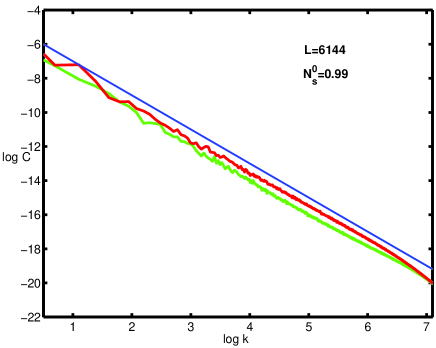
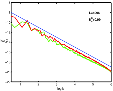
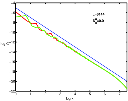
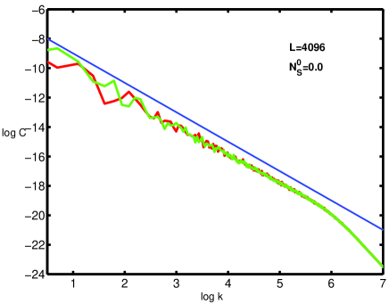
Figure 1: Log-log plots of $C_{hh}(k)$ (red) and $C_{\phi\phi}(k)$ (green) versus $k$ for $L=6144$ with $N_{s}^{0}$=0.9 ($N_{s}=0.82$) (top left) and $N_{s}=N_{s}^{0}=0.0$ (bottom left), and for $L=4096$ with $N_{s}^{0}$=0.9 ($N_{s}=0.81$) (top right) and $N_{s}=N_{s}^{0}=0.0$ (bottom right). The blue line, drawn as a guide to the eye, indicates a slope of -2, corresponding to the value $\chi_{h}=1/2$ for the roughness exponent for the fields $h$ and $\phi$. Note that at finite $N_{s}$ there are amplitude differences between the scaling regimes of $C_{hh}(k)$ and $C_{\phi\phi}(k)$ (top plots) where as for $N_{s}^{0}=0.0$ the amplitude differences disappear (bottom plots) (see text).

We now show the time-dependence of the widths $W_{h}(t)$ and $W_{\phi}(t)$ in Fig. (2) for system size $L=4096$. We notice that the saturated amplitude difference between $W_{h}(t)$ and $W_{\phi}(t)$ increases as $N_{s}^{0}$ increases from 0.0 to 0.9. Since the ratio of the saturated amplitudes of $W_{h}(t)$ and $W_{\phi}(t)$ yields the ratio $A$ ($W_{\phi}/W_{h}=\sqrt{A}$), we find that $A$ decreases as $N_{s}^{0}$ increases. This is in accordance with the results as presented in Fig. (1).

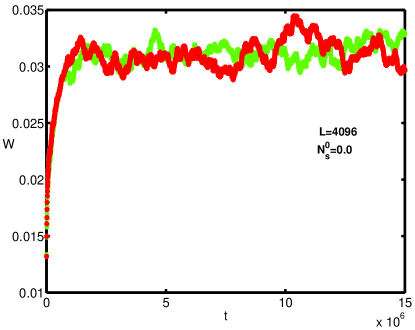
Figure 2: A plot of the widths $W_{h}(t)$ (red) and $W_{\phi}(t)$ (green) versus time $t$ for system size $L=4096$ with $N_{s}^{0}=0.0,\,0.9$ from our $1d$ DNS studies. Clearly the saturated amplitude difference increases as $N_{s}^{0}$ increases.

Figure (3) shows the dependence of the parameter $A$ obtained from the plots above on $N_{s}^{0}$ for system sizes $L=2048,4096,6144$. We find that the amplitude-ratio $A$ decreases monotonically as $N_{s}^{0}$ increases in agreement with the behavior of our mode coupling analyses. We do not observe any noticeable systematic dependence of this behavior on system sizes. Therefore, results from our $1d$DNS studies agree with those from the analytical studies mentioned above.

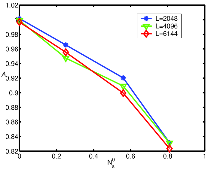
Figure 3: A plot of the parameter $A$ versus $N_{s}^{0}$ for our $1d$ DNS studies for system sizes $L=2048,4096,6144$. The general trend that $A$ decreases with an increase in $N_{s}^{0}$ is observed for the all system sizes we worked with.

5.1.2 Results in two dimensions:

In this Section we present our results from our $2d$ DNS of the model Eqs. (14) and (15) and compare with the analytical results already obtained. In our DNS studies (using pseudo-spectral methods) in $2d$ the system sizes we work with are $96^{2}$, $128^{2}$ and $160^{2}$. Unlike in $1d$, the system exhibits a non-equilibrium phase transition from a smooth phase, characterized by logarithmic roughness ($\chi_{h}=0$) and $\alpha$ independent of $N_{s}^{0}$, to a rough phase characterized by algebraic roughness ($\chi_{h}\geq 0$) and a decreasing $A$ as $N_{s}^{0}$ increases. In the smooth phase, $A$ is fully determined by the bare ratio $D_{b}^{0}/D_{u}^{0}$. Therefore, a simple way of ascertaining which phase the system is in, is by measuring $A$.

In our $2d$DNS studies there two tuning parameters to reach the rough phase of the system. They are $D_{u}^{0}$ and $N_{s}^{0}$. The crossover from the smooth-to-rough phases is formally determined by the value of the coupling constant $G=\lambda D_{u}^{2}/\nu^{3}$ (see above). Here the renormalized parameter $D_{u}$ has a monotonic dependence on the bare amplitude $D_{u}^{0}$. For small $D_{u}^{0}$, renomalized $G$ is zero and the system is in its smooth phase. With increasing $D_{u}^{0}$ the system eventually crosses over to the rough phase where various values of $\alpha$ have been obtained by tuning $N_{s}^{0}$. For each system size we obtain the widths $W_{h}(t)$ and $W_{\phi}(t)$ as a function of time $t$. As for the height field in the well-known KPZ equation plots of $W_{h}(t)$, as a function of time, have a growing part and a saturated part. The system size dependences of the saturation values of the widths $W_{h}(t)$ and $W_{\phi}(t)$ yield the values of the roughness exponents of the corresponding fields. Since we are interested in the statistical properties of the rough phase, in our $2d$DNS studies we access this phase by sufficiently large $D_{u}^{0}$ for reasons as explained above. As shown below, we find $A<1$ for non-zero $N_{s}^{0}$. This ensures that we are indeed able to access the rough phase in our DNS runs. We present our results from system sizes $96^{2}$ and $128^{2}$ in Fig. (4) for two values of the parameter $N_{s}^{0}=0.0,\,0.9$ for each system size. The data from $160^{2}$ runs show similar behavior. We determine $A$ and the ratio $\chi_{h}/z$. Note that for each system size the amplitude differences differences between the saturation values of the widths $W_{h}(t)$ and $W_{\phi}(t)$ (i.e., the parameter $A$ in Sections 4.2 and 4.3) increase monotonically with $N_{s}^{0}$, in agreement with our SCMC and FRG analyses. Such nontrivial dependence of $A$ on $N_{s}^{0}$ is a key signature of the rough phase.

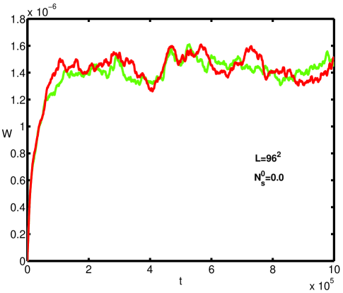
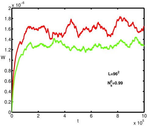
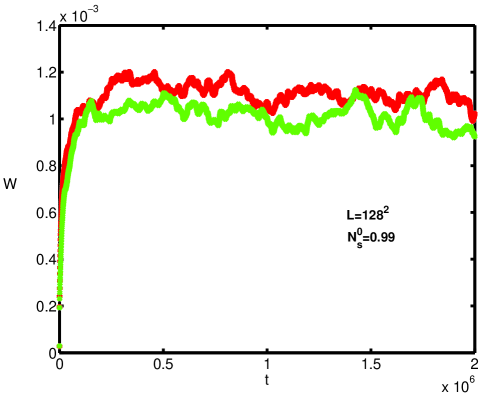
Figure 4: Plots of $W_{h}(t)$ (red) and $W_{\phi}(t)$ (green) versus $t$ in the rough phase for the system sizes $96^{2}$ (top) and $128^{2}$ (bottom) for $N_{s}^{0}=0.0,\,0.9$. Note the increasing differences between the saturation values of $W_{h}$ and $W_{\phi}$ with increasing $N_{s}^{0}$.

From our DNS studies with system sizes $96^{2},\,128^{2},\,160^{2}$ we calculate the parameter $A$. We show its dependence on $N_{s}^{0}$ in the Fig. (5). As in $1d$ we see that $A$ decreases monotonically as $N_{s}^{0}$ increases from zero.

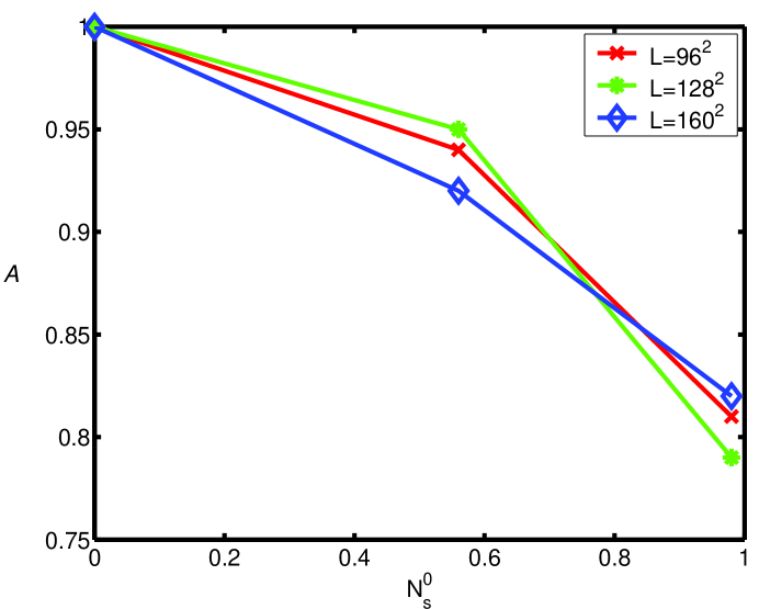
Figure 5: A plot of $A$ versus $N_{s}^{0}$ for various system sizes from our $2d$DNS studies.

We now determine the scaling exponents $\chi_{h}$ and $z$. Due to the very time consuming nature of the $2d$ simulations the quality of our data for $2d$ are much poorer than those obtained from our $1d$ runs. Because of this difficulty we do not extract the roughness exponent directly by plotting different correlation functions in the steady state as functions of wavevector $k$. Instead we obtain the ratio $\chi_{h}/z$ by plotting the width $W_{h}(t)$ as a function of time $t$ in a log-log plot for $t\lesssim$ saturation time scale. The slope yields the ratio $\chi_{h}/z$; we obtain $\chi_{h}/z=0.2\pm 0.1$ which is to be compared with our analytical result $1/5$, obtained by means of SCMC and FRG calculations. At $d=2$ SCMC yields $z=1.66$ which is close to Ref. [29] whereas our DNS yields $z\approx 1.60\pm 0.1$. Numerical studies of our type, performed on bigger system sizes, should be able to yield highly accurate values for the scaling exponents which could be compared systematically with our SCMC/FRG results and those of Ref. [29]. However, we refrain ourselves from making such detailed comparisons due to the rather small system sizes we have worked with. We present our result in Fig.6 below for the system sizes $L=128^{2}$ and $L=160^{2}$ with $N_{s}^{0}=0.0$ and $N_{s}^{0}=0.9$ respectively. Note that, within the accuracy of our numerical solutions, the ratio $\chi_{h}/z$ does not depend upon the value of $N_{s}^{0}$, suggesting that the scaling exponents are independent of symmetric cross-correlations in agreement with our SCMC (Section 4.3) and FRG (Section 4.4) above.

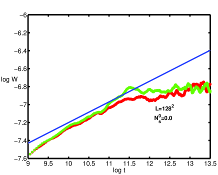
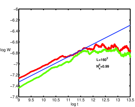
Figure 6: Log-log plots of $C_{hh}(k,t=0)$ and $C_{\phi\phi}(k,t=0)$ versus $k$ from our $2d$DNS studies: (i) $L=128^{2},\,N_{s}^{0}=0.0$, (ii) $L=160^{2},\,N_{s}^{0}=0.9$. The slope $\sim 0.2$ yields $\chi_{h}/z$ (see text).

We conclude this Section by summarizing our results. We performed DNS of the model Eqs. (14) and (15) at $d=1,\,2$ in the presence of the symmetric cross-correlations parametrised by $N_{s}^{0}$. By tuning the bare amplitude $D_{0}$ we are able to access the rough phase in $2d$. In both dimensions we find that in the rough phase the ratio $D_{b}/D_{u}$ decreases monotonically from unity as $N_{s}^{0}$ increases from zero. In $1d$ we find $\chi_{h}=0.5$ very accurately which is in good agreement with the analytically obtained results. In $2d$ we find $\chi_{h}/z=0.2\pm 0.1$ which is to be compared with our analytical estimate of 1/5. Extensive DNS studies on larger system sizes would be required to calculate the scaling exponents with high accuracy.

5.2 Monte Carlo simulations of the coupled lattice-gas models in one dimension

So far in the above we have studied the applications of several methods, analytical as well numerical, on the continuum model Equations (9) and (10) [or Eqs. (14) and (15)] and obtained several results concerning universal properties of the statistical steady-state of the model. Note that all techniques used above have been applied on the same model. To complement our studies we discuss the results from the lattice-gas model in this section which we constructed [see Section 3], and compare with our results already obtained above.

In this section we simulate our proposed one-dimensional lattice-gas models for the model Eqs. (21). By using relations (23) we calculate the ratios of appropriate correlation functions in the steady state. We use Monte Carlo methods to simulate our models. We extended the Restricted-Solid-On-Solid (RSOS) algorithm [20] and the Newman-Bray (NB) algorithm [22] for the KPZ surface growth phenomena to construct the coupled lattice-gas models in $1d$ for Eqs. (21) with cross-correlations. In such models particles are deposited randomly from above and settle on the already deposited layer following certain growth rules which define the models. One typically measures the widths of the height fluctuations of the growing surfaces as functions of time $t$. Note that our numerical works on the lattice-gas models are restricted to lattices of modest sizes ($L=4096$ is the largest system size considered). This is due to the fact that the numerical generation of noise cross-correlations of the type we considered is not uncorrelated in space in $1d$, rather it has a variance proportional to $1/x$. Generation of such noises is a very time consuming process: we first generate the noises in the real space. These are uncorrelated Gaussian random noises without any cross-correlations. We then bring them to Fourier space by Fourier transform. Inverse Fourier transforms of particular linear combinations of them yield noises with finite cross-correlations which we use in our studies. Although we have used Fast Fourier Transforms, they are still computationally rather time consuming and hence reduce the over all speed of the code. In contrast, the more common lattice-gas studies on the KPZ equation do not require Fourier Transforms of the noise (since they do not have any noise cross-correlations) and hence are much faster. This allows them to study up to much larger system sizes.

5.2.1 A coupled lattice-gas model in one dimension with RSOS update rules:

The restricted solid-on-solid (RSOS) update rules involve selecting a site on the lattice randomly and permitting growth by letting the height of the interface at the chosen site increase by unity such that the height difference between the selected site and the neighbouring sites does not become more than unity [20]. Our model involves two sublattices where the height fields on each of the sublattices satisfy each of Eqs. (21). In our coupled lattice model each sublattice is evolved according to the RSOS update rule described above. The selection of the random sites in the two sublattices may be correlated. This correlation models the noise cross-correlations of the model continuum Eqs. (9) and (10) or (21).

We simulated our coupled lattice-gas model described above and calculate the widths $W_{h}(t),\;W_{\phi}(t)$ of the growing surfaces $h(x,t)$ and $\phi(x,t)$ as functions of time $t$. Similar to the single-component KPZ equation, the plots have two distinct parts - an initial growing part and a late time saturated part. Below we present our results graphically: We plot $W_{h}(t)$ (red) and $W_{\phi}(t)$ (green) versus $t$ for system size $1024$ in Fig. (7). Results from system sizes $L=2048,\,4096$ show similar behavior without any systematic system size dependence.

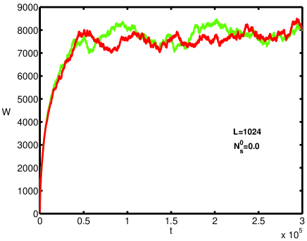
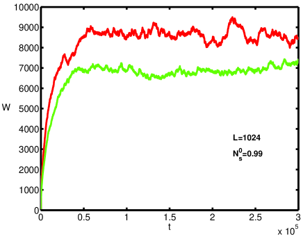
Figure 7: Plots of $W_{h}(t)$ (red) and $W_{\phi(t)}$ (green) versus $t$ for system size $L=1024$ for $N_{s}^{0}=0.0,\,0.9$ in our coupled lattice-gas model based on the RSOS algorithm. Note the increasing difference between $W_{h}$ and $W_{\phi}$ with increasing $N_{s}^{0}$.

In Fig. 8 we present a plot of $A$ versus $N_{s}^{0}$ for the system sizes $L=1024,\,2048,\,4096$. As in our results obtained analytically and DNS, $A$ decreases monotonically from unity as $N_{s}^{0}$ increases from zero. We do not observe any systematic system size dependence.

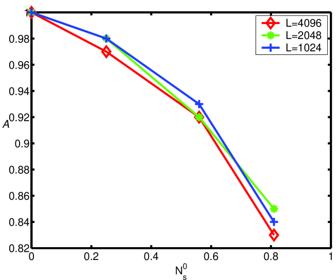
Figure 8: A plot of $A$ versus $N_{s}^{0}$ for various system sizes obtained from numerical simulations of our coupled lattice-gas models with the RSOS algorithm.

Having shown the dependence of $A$ on $N_{s}^{0}$ we now estimate the scaling exponents $\chi_{h}$ and $z$ to complete the discussions on the universal properties of the lattice-gas model. Below we present a log-log plot of the equal-time correlation function $C_{hh}(k)\equiv\langle h(k,t)h(-k,t)\rangle$ in the steady state as a function of the Fourier vector $k$ [Fig. (9)]. We find that slope in the scaling regime (small $k$) is very close to -2 corresponding to $\chi_{h}=1/2$ as predicted by analytical means before.

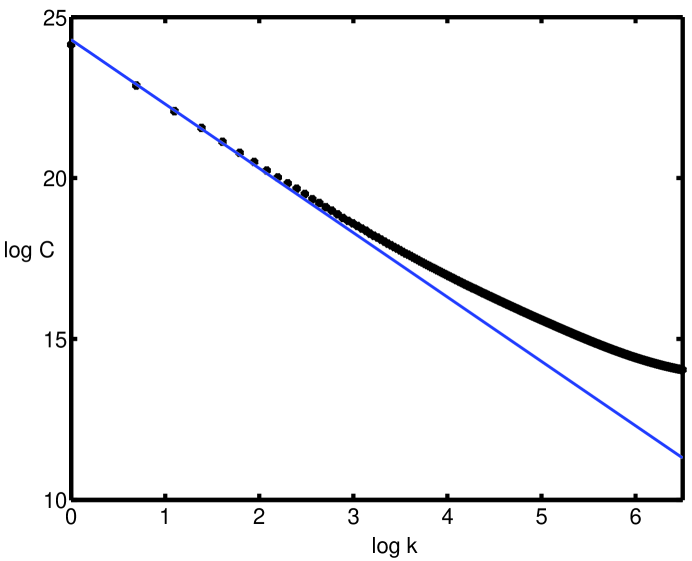
Figure 9: A log-log plot of the correlation function $C_{hh}(k)$ versus $k$ for system size $L=2048$ from our coupled lattice-gas model with the RSOS algorithm. The straight line with a slope of -2, corresponding to $\chi_{h}=1/2$, represents the scaling regime of $C_{hh}(k)$ for small $k$ (long wavelength limit).

An alternative way to obtain the scaling exponent $\chi_{h}$ is by finding the dependence of the saturated value of the widths $W_{h}(t)$ and $W_{\phi}(t)$ on the system size $L$. Since, after saturations in the steady states $W_{h,\phi}\sim L^{2\chi_{h}}$ with $L$ being the system size, we obtain $\chi_{h}$ from the slope of the plots of logarithm of the saturated values of the widths versus logarithm of the corresponding system sizes. We find $\chi_{h}=0.49\pm 0.05$ which is very close to the analytically obtained value, Further, from the time-dependences of the widths $W_{h}(t)$ and $W_{\phi}(t)$ the exponent-ratio $\chi_{h}/z$ can be obtained. Fig. 10 shows a log-log plot of $W_{h}(t)$ and $W_{\phi}(t)$ versus $t$ from a lattice size $L=16384$. For such a large lattice size the saturation time is very large and hence we show only the growing part of the curves. The slope yields the ratio $\chi_{h}/z$. The red and green points refer to $W_{h}(t)$ and $W_{\phi}(t)$, and the blue line a slope of $0.32$ indicating $\chi_{h}/z=0.32$ which is very close to the analytically obtained value of $1/3$. In short, therefore, the results from the Monte-Carlo simulations of our coupled lattice-gas model in $1d$, based on the RSOS algorithm, yield results in close agreement with those obtained through analytical means and $1d$DNS.

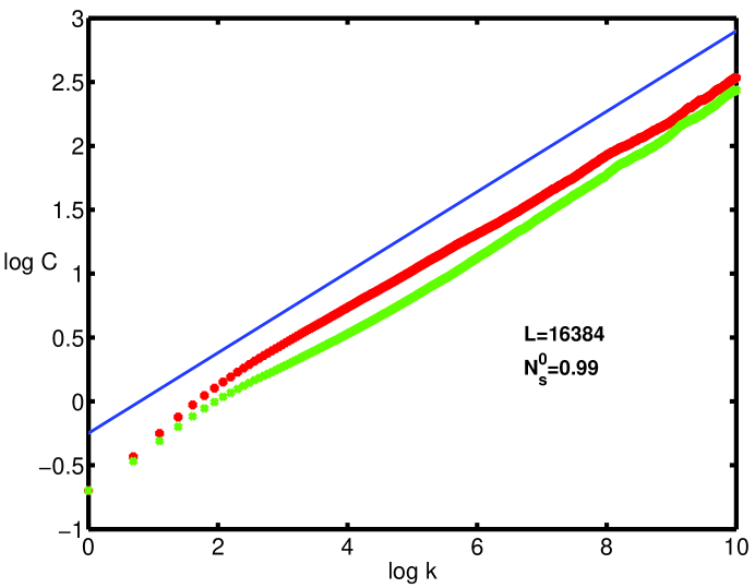
Figure 10: A log-log plot of $W_{h}(t)$ (red) and $W_{\phi}(t)$ (green) versus $t$, obtained from our lattice-gas model with the RSOS algorithm with system size $L=16384$. The black line indicates a slope of 0.32 for easy eye estimation.

5.2.2 A coupled lattice-gas model in one dimension with the NB update rule:

As mentioned before, this model uses the mapping between the KPZ surface growth problem and the equilibrium problem of a directed polymer in a random medium (DPRM) which are connected by the non-linear Cole-Hopf transformation $h_{1,2}({\bf x},t)=(2\nu/\lambda)\ln Z_{1,2}$ leading to the Eqs.(70) for the partition functions $Z_{1,2}$ for the two DPs. Further, one uses the following update rules for $h_{1,2}$:

$$\tilde{h}_{i}(t) = h_{i}(t)+\Delta^{1/2}\zeta_{i}(t),$$

$$h_{i}(t+\Delta) = \tilde{h}_{i}(t)+(\nu/\lambda)\ln\left[1+(\Delta\nu/a^{2})\Sigma_{jnni}[e^{\lambda(\tilde{h}_{j}-\tilde{h}_{i})/\nu}-1]\right],$$ (89)

where $\Delta$ and $a$ are the grid scales for time and space, respectively, and $jnni$ indicates sites $j$ and $i$ being nearest neighbors. Then, taking the strong coupling limit $\lambda\rightarrow\infty$ one finally obtains

$$h_{i}(t+\Delta)={\rm max}_{jnni}(\tilde{h}_{i},\{\tilde{h}_{j}\}).$$ (90)

This is same as the zero-temperature DPRM algorithm, written in terms of the fields $h_{1,2}$. We implement the above growth rule in $1d$ with system sizes $L=1024,2048,4096$. Functions $W_{h}(t)$ and $W_{\phi}(t)$, as defined in Sec.5.2.1 are obtained by taking appropriate linear combinations of the equal-time correlators of $h_{1,2}$. We present our results graphically in Fig. (11) for system size $L=1024$ below.

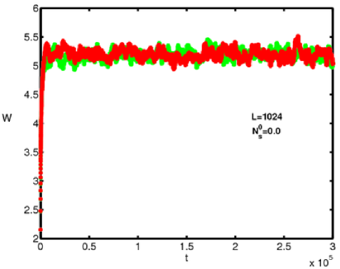
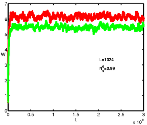
Figure 11: Plots of $W_{h}(t)$ (red) and $W_{\phi}(t)$ versus $t$ for system size $L=1024$ for various $N_{s}$ in our coupled lattice-gas model based on the NB algorithm (see text). Note the increasing difference between $W_{h}$ and $W_{\phi\phi}$ with $N_{s}^{0}=0.0,\,0.55,\,0.9$.

From Fig. (11) it is clear that after saturations, the differences between $W_{h}$ and $W_{\phi}$, measured by $A$, increase with $N_{s}^{0}$. Below in Fig. (12) we show a plot depicting the variation of $A$ versus $N_{s}^{0}$ obtained from the simulations of our coupled lattice-gas model with the NB update rule in $1d$. As before, we find that $A$ decreases monotonically from unity as $N_{s}^{0}$ increases from zero.

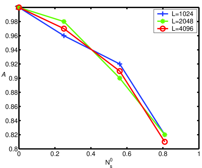
Figure 12: A plot of $A$ versus $N_{s}^{0}$ obtained from numerical solutions of our coupled lattice-gas model with the NB update rule for system sizes $L=1024,\,2048,\,4096$ in $1d$.

We further determine the scaling exponents $\chi_{h}$ and $z$ from our numerical results, as we did above in Section 5.2.1. Fig. (13) shows a log-log plot of $W_{h}(t)$ and $W_{\phi}(t)$ versus $t$ for the system size $L=4096$. We find that the initial slope is $0.32\pm 0.02$ which is very close to the analytically obtained $\chi_{h}/z=1/3$.

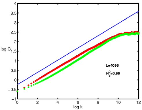
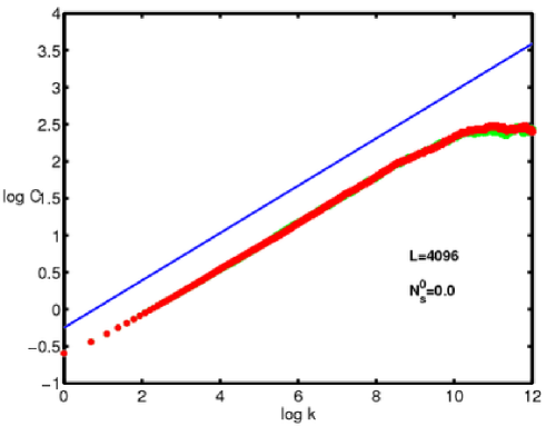
Figure 13: Log-log plots of $W_{h}(t)$ (red) and $W_{\phi}(t)$ (green) versus $t$ for system size $L=4096$ with $N_{s}^{0}=0.99$ (left) and $N_{s}^{o}=0.0$ (right) respectively. These are obtained from our lattice-gas model with the NB algorithm The initial slopes are very close to the analytically obtained value (see text).

Furthermore, the equal-time correlation function $C_{hh}(k,0)$ as a function of $k$ is shown in a log-log plot [Fig. 14]. We find that in the scaling regime (small $k$) $k^{-2}$ is an excellent fit for $C_{hh}(k)$ yielding $\chi\simeq 1/2$. This, together with the fact that $\chi_{h}/z\simeq 1/3$ give $z\simeq 3/2$, close to what we estimated by other means in $1d$ as reported above.

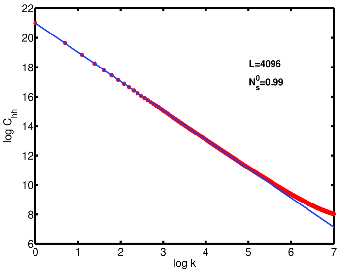
Figure 14: A log-log plot of $C_{hh}(k)$ versus $k$ from simulations of our coupled lattice-gas model with the NB algorithm (L=4096). The black line is a guide to slope -2 which agrees very well with our data in the scaling (small $k$) region.

We close this section by summarizing our results from the Monte-Carlo simulations of the two lattice-gas models proposed by us. Both the models, based on the RSOS and the NB algorithms respectively, exhibit similar dependence of the parameter $A$ over $N_{s}^{0}$. They further yield the same scaling exponents. All these are in close agreements with our analytical results obtained from DRG/SCMC/FRG methods as well as $1d$DNS studies.

5.3 Lattice-gas models and the continuum equations of motion: Universality for systems out of equilibrium

In the above we have obtained results on the scaling exponents and the correlation functions in the statistical steady states from different approaches. In particular we compare our results in $1d$ on the dependence of the amplitude ratio $A$ on the symmetric cross-correlations $N_{s}^{0}$ from the numerical solutions (DNS) of the continuum model Eqs. (9) and (10), and the numerical simulations of the lattice-gas models based on the RSOS and NB algorithms. Since in none of the cases we considered we find any systematic system-size dependence, we take average of our results from different system sizes for the same value of $N_{s}^{0}$ for a given type of study (DNS/NB/RSOS). We present our results in a composite plot (15) below.

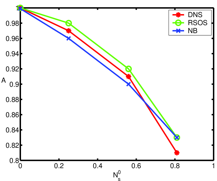
Figure 15: A plot showing the variation of the amplitude ratio $A$ as a function of the symmetric cross-correlations $N_{s}^{0}$ (see text) in $1d$ from RSOS (red x), NS (green *) and DNS (blue diamond).

We find that the general trend that the ratio $A$ decreases from unity when $N_{s}^{0}$ increases from zero persists in all the cases. Moreover, all the cases yield values of the scaling exponents which are very close to each other and in close agreement with the analytically obtained values as well.

6 Summary and outlook

We have considered the statistical properties of the generalized Burgers model (GBM) egiven by equations (9) and (10), driven by conserved zero-mean Gaussian noise sources with variances (17, 18) and (19). We have undertaken a variety of analytical and numerical investigations to uncover the universal properties of the correlation functions in $d$ dimensions.

Upon employing analytical approaches like DRG, FRG and SCMC we have calculated the scaling exponents and the amplitude ratios at $d=1$ and at $d\geq 2$. Each of these methods have a certain range of applicability and also limitations. The DRG method yields results only for the strong coupling phase in $d=1$ and the unstable critical point (for $d>2$), for both symmetric and antisymmetric cross-correlations. The FRG method works for the strong coupling phases at $d=1$. For $d>2$ it is able to capture the physics in the strong coupling phase, but only for symmetric cross-correlations. The SCMC method is useful to study the strong coupling phases at $d=1$ and $d>2$ for both symmetric and anti-symmetric cross-correlations. Taking all the methods from the various analytical methods together a coherent picture emerges. We broadly find that symmetric cross-correlations affect the amplitude ratio and the anti-symmetric cross-correlations affect the scaling exponents. Since, in general, both symmetric and the anti-symmetric cross-correlations are likely to be present, one may encounter scaling exponents and amplitude ratios varying with the strength of cross-correlations. In addition to our analytical studies, we have performed extensive numerical work in $1d$. We have numerically solved the continuum model equations using the pseudo-spectral method in one and two dimensions, and numerically simulated two equivlent lattice-gas models in $1d$. In all the cases we numerically calculated the equal-time correlation functions of the two height fields $h$ and $\phi$, and measured their spatial scaling exponents and the amplitude ratios. Our numerical results on the scaling exponents agree very well with those obtained analytically for $d=1$. Further, our results on the dependence of the amplitude-ratio on the strength of the cross-correlations from the numerical studies agree broadly with those from the analytical studies.

In $2d$ we have numerically solved the continuum model equations (14) and (15) in the presence of symmetric cross-correlations only. The amplitude ratios display dependences on the cross-correlations similar to those obtained analytically. We also obtained scaling exponents numerically. Due to the difficult nature of the $2d$ simulations these are less accurate than their $1d$ counterparts. Since we use a pseudo-spectral code, our method is free from the controversial issue of real-space discretization [35]. Owing to the small system sizes and the high saturation time for the widths, the quality of our data are less satisfactory than those obtained from our $1d$ models. We are only able to measure the ratio $\chi_{h}/z$ from our numerical studies in $2d$. Nevertheless, the effects of noise cross-correlations have qualitatively the same effects on the amplitude ratio. Detail studies to yield the scaling exponents in $2d$ with high accuracy will be presented elsewhere [36].

Our results potentially have broad implications for natural systems with coupled degrees of freedom. There are many such examples - MHD turbulence, turbulence in a binary fluid mixture, biologically relevant systems, e.g., coupled TASEPs (Totally Asymmetric Exclusion Process) modeling transports in cellular systems, dynamics of motors and microtubules, dynamics of visco-elastic active polar gels etc. The general conclusions of our investigations, namely, the relevance of the strength and the symmetry of the cross-correlations in determining the long wavelength properties, are expected to be visible in such systems as well, although detailed accounts are likely to depend on the systems in question. To test our predictions experimental measurements should include correlation functions and effective transport coefficients. These are likely to be affected by the presence of cross-correlations. In driven fluid-like turbulent systems (MHD, binary fluid mixtures) cross-correlations can be experimentally controlled by tuning the external (stochastic) forces. In such systems one needs to measure correlation functions of velocity and magnetic fields (in MHD) or velocity and concentration gradient fields (in binary fluid mixtures) in the scaling limit and obtain the scaling exponents characterizing the correlation functions in the hydrodynamic limit as functions of the amplitudes of the cross correlation functions.

7 Acknowledgement

A part of the work was done when one of the authors (AB) was working at the Hahn-Meitner-Institut, Berlin as a Humboldt Fellow. AB wishes to thank the Alexander von Humboldt Stiftung, Germany for partial financial support. AB also thanks SERC (DST, India) for partial financial support through a grant under the Fast Track Scheme SR/FTP/PS-17/2006. Some of the computational works have been done using the computational resources of Centre for Applied Mathematics and Computer Science (CAMCS), SINP. AB thanks CAMCS for making such facilities available for this work and for partial financial support.

8 Glossary

For the convenience of the reader we provide below a list of symbols for the functions and parameters which are used in the bulk of the article.

• ${\bf u}({\bf x},t),\;\;{\bf b}({\bf x},t)\Rightarrow$ Burgers fields.

• ${\bf z}^{\pm}={\bf u\pm b}\Rightarrow$ Elsässer   variables.

• ${\bf u}=\nabla h,\,{\bf b}=\nabla\phi$. Fields $h$ and $\phi$ are (non-conserved) height variables.

• ${\bf z^{\pm}}=\nabla h_{1,2}$, $h_{1,2}$ are (non-conserved) height fields; $h_{1,2}$ also represent the free energies of two (identical) directed polymer in a random medium; $h_{1,2}=\frac{1}{2}(h\pm\phi)$.

• $\nu_{0},\,\mu_{0}\Rightarrow$ Bare (unrenormalized) viscosities for the fields $\bf u$ and $\bf b$; $\nu,\,\mu\Rightarrow$ Renormalized fluid and magnetic viscosities.

• $\lambda_{1},\,\lambda_{2},\,\lambda_{3}\Rightarrow$ coupling constants. They are set to unity in most of what follows.

• $G_{u,b}({\bf k},\omega)\Rightarrow$ Renormalized propagators/response functions of the fields $\bf u$ and $\bf b$.

• $\Sigma({\bf k},\omega)\Rightarrow$ Self-energy function of $\bf u$ and $\bf b$; $\Gamma\Rightarrow$ amplitude of $\Sigma({\bf k},0),\,\Gamma=\nu=\mu$ in the present model.

• $C^{u}_{ij},\,C^{b}_{ij},\,C^{\times}_{ij}\Rightarrow$ Auto correlation functions of $\bf u$ and $\bf b$, and cross correlation function respectively, $i,j\Rightarrow$ Cartesian indices.

• $D_{u}^{0},\,D_{b}^{0}\Rightarrow$ Bare amplitudes of the auto-correlations of the external Gaussian noise sources in the $\bf u$ and $\bf b$ equations [Eqs. (9,9)]; $D_{u},\,D_{b}\Rightarrow$ corresponding renormalized (scale-dependent) amplitudes.

• $D_{s}^{0},\,D_{a}^{0}\Rightarrow$ Bare amplitudes of the symmetric and anti-symmetric parts of the noise cross-correlations in Eqs. (9,9); $D_{s},\,D_{a}\Rightarrow$ corresponding renormalized amplitudes.

• $P_{m}=\nu/\mu\Rightarrow$ Renormalized Prandtl number.

• $A=D_{b}/D_{u}\Rightarrow$ Dimensionless renormalized amplitude ratio.

• $N_{s}^{0}=(D_{s}^{0}/D_{u}^{0})^{2},\,N_{s}=(D_{s}/D_{u})^{2}$, $N_{a}=(D_{a}/D_{u})^{2}$.

• $D_{0}=D_{u}^{0}+D_{b}^{0},\;\hat{D}=D_{u}^{0}-D_{b}^{0}$.

• $V_{1},V_{2}\Rightarrow$ Random potentials embedding directed polymers (DP) A and B.

• $Z_{1},Z_{2}\Rightarrow$ Partition functions of DP A and B.

• $R_{1},R_{2},\tilde{R},\hat{R}\Rightarrow$ Different variances of the random potentials $V_{1}$ and $V_{2}$.

• $\Gamma_{0}=\left[\frac{R_{\times}({\bf x})}{R_{1}({\bf x})}\right]^{2},\,\gamma=\frac{\hat{R}({\bf x})}{R_{1}({\bf x})}$. Since, $R_{1}({\bf x}),\,\hat{R}({\bf x}),\,R_{\times}({\bf x})$ have same scaling behavior in the hydrodynamic limit, $\gamma,\,\Gamma_{0}$ are constants. To the lowest order $\Gamma_{0}=N_{s},\,\gamma=A$.

• $G=\frac{\lambda^{2}D_{u}}{\nu^{3}}\Rightarrow$ Dimensionless coupling constant in one-loop dynamic renormalization group calculations in the presence of symmetric cross-correlations; $G_{a}=\frac{\lambda^{2}D_{u}}{\nu^{3}}\Rightarrow$ the same for anti-symmetric cross-correlations.

• $\tilde{\Gamma}\Rightarrow$ Vertex generating functional.

• $\epsilon=2-d$ where $d$ is the physical space dimension.

• $\chi_{u},\,\chi_{b},\,z\Rightarrow$ Two roughness and dynamic scaling exponents respectively of the fields $\bf u$ and $\bf b$. In the model here, $\chi_{u}=\chi_{b}=\chi,\,\chi+z=1$.

• $\chi_{h},\,\chi_{\phi}\Rightarrow$ Roughness exponents of $h$ and $\phi$; $\chi_{h}=\chi_{\phi},\,\chi_{h}+z=2$.

• $\zeta=1/z\Rightarrow$ scaling exponent characterizing the scaling of transverse fluctuations of directed polymer with its longitudinal length.

• $T=1/\nu_{0}\Rightarrow$ Temperature of a DP in a random medium.

9 Appendix

9.1 Symmetries and Ward identities

In this section we elucidate the continuous symmetries under which the equations of motion (9) and (10) remain invariant. These allow us to construct exact relations between different vertex functions which in turn impose strict conditions on the renormalization of different parameters in the model.

We begin by rewriting the Eqs.(9) and (10) by expressing the Burgers $\bf b$-fields (whose mean value is always kept zero here and below) as a sum of a constant vector and a space-time dependent part, i.e., splitting the fields ${\bf b}({\bf x},t)\rightarrow{\bf b}({\bf x},t)+{\bf B_{0}}/\lambda_{2}$ where ${\bf B_{0}}/\lambda_{2}$ is a constant vector:

$${\partial{\bf u}\over\partial t}+\nabla{\bf B_{0}\cdot b}+\lambda_{1}\nabla{u}^{2}+\lambda_{2}{\nabla b^{2}}=\nu_{0}\nabla^{2}{\bf u}+{\bf f}$$ (91)

and

$${\partial{\bf b}\over\partial t}+(\lambda_{3}/\lambda_{2})\nabla{\bf B_{0}\cdot u}+\lambda_{3}{\bf\nabla(u\cdot b)}=\mu_{0}\nabla^{2}{\bf b}+{\bf g}.$$ (92)

In this notation the mean Burgers $\bf b$-field is $\langle{\bf b}\rangle+{\bf B_{0}}=0$.

The generating functional corresponding to Eqs. (9) and (10) is written as [37, 38] $Z[{\bf j_{1},\hat{j}_{1},j_{2},\hat{j}_{2}}]=\int Du_{i}D\hat{u}_{i}Db_{i}D\hat{b}_{i}\exp[{\mathcal{S}}]$ [39], where the action functional $\mathcal{S}$ is given as

$${\mathcal{S}}[\Phi] = -\int\hat{b}_{i}\hat{b}_{j}D^{b}_{ij}-\int\hat{u}_{i}\hat{u}_{j}D^{u}_{ij}-i\int\hat{u}_{i}\hat{b}_{j}{D_{\times}}_{s}-i\int\hat{u}_{i}\hat{b}_{j}\varepsilon_{ijp}k_{p}i{D_{\times}}_{a}$$ (93)

$$-i\int\hat{u}_{i}[\partial_{t}u_{i}+\frac{\lambda_{1}}{2}\nabla u^{2}+\frac{\lambda_{2}}{2}\nabla b^{2}+\nabla{\bf B_{0}\cdot b}-\nu_{0}\nabla^{2}u_{i}]$$

$$- i\int\hat{b}_{i}[\partial_{t}b_{i}+\lambda_{3}\nabla({\bf u\cdot b})+(\lambda_{3}/\lambda_{2})\nabla{\bf B_{0}\cdot u}-\eta_{0}\nabla^{2}b_{i}].$$

From the dynamic generating functional one obtains the vertex generating functional $\Gamma$ [39] through

$$\tilde{\Gamma}[u_{i},\hat{u}_{i},b_{i},\hat{b}_{i}]=W[j_{i},\hat{j}_{i},l_{i},\hat{l}_{i}]-\int j_{i}u_{i}-\int\hat{j}_{i}\hat{u}_{i}-\int l_{i}b_{i}-\int\hat{l}_{i}\hat{b}_{i},$$ (94)

where $W=\ln Z$ is the generator of the connected diagrams and $\tilde{\Gamma}$ is the generator of the one-particle irreducible diagrams [40].

The equations of motion (9) and (10) or the action functional given by (93) are invariant under the following transformations:

• The Galilean transformation (TI): ${\bf u}({\bf x},t)\rightarrow{\bf u}({\bf x+u_{0}}t,t)+{\bf u_{0}},\;\frac{\partial}{\partial t}\rightarrow\frac{\partial}{\partial t}-\lambda{\bf u_{0}}.\nabla,$ and ${\bf b}\rightarrow{\bf b}$ [6, 15, 41] with $\lambda_{1}=\lambda_{3}=\lambda$ in Eqs. (91) and (92. This implies, as we show below, non-renormalization of $\lambda_{1}$ [6, 15, 23].

• The transformation TII: ${\bf B_{0}\rightarrow B_{0}}+\lambda_{2}\delta$, ${\bf b}({\bf x},t)\rightarrow{\bf b}({\bf x},t)-{\bf\delta}$, $\bf u\rightarrow u$. Here the shift $\delta$ is a vector.

Let us first consider the invariance under the Galilean transformation TI and the corresponding Ward identities. The invariance of the vertex generating functional $\tilde{\Gamma}$ yields

$$\tilde{\delta}\Gamma = {\bf u_{0}}\cdot\int_{\bf q}\int dti\lambda{\bf q}t[\frac{\delta\tilde{\Gamma}}{\delta u_{j}({\bf q},t)}u_{j}({\bf q},t)+\frac{\delta\tilde{\Gamma}}{\delta\tilde{u}_{j}({\bf q},t)}\tilde{u}_{j}({\bf q},t)$$ (95)

$$+ \frac{\delta\tilde{\Gamma}}{\delta b_{j}({\bf q},t)}b_{j}({\bf q},t)+\frac{\delta\tilde{\Gamma}}{\delta\tilde{b}_{j}({\bf q},t)}\tilde{b}_{j}({\bf q},t)]$$

$$+ {\bf u_{o}}\cdot\int_{\bf q}\int dt\delta({\bf q})\frac{\delta\tilde{\Gamma}}{\delta{\bf u}({\bf q},t)}=0.$$

By taking functional partial derivatives with respect to different fields we obtain (in time space)

$$\lambda(q_{i}^{\prime}t^{\prime}+q_{i}^{\prime\prime}t^{\prime\prime})\tilde{\Gamma}_{\tilde{u}_{j}u_{k}} = -\int dt\tilde{\Gamma}_{\tilde{u}_{j}u_{i}u_{k}}({\bf q^{\prime}},t^{\prime};{\bf-q^{\prime}},t^{\prime\prime};{\bf q},t)|_{{\bf q}=0},$$ (96)

$$\lambda(q_{i}^{\prime}t^{\prime}+q_{i}^{\prime\prime}t^{\prime\prime})\tilde{\Gamma}_{\tilde{u}_{j}\tilde{u}_{k}} = -\int dt\tilde{\Gamma}_{\tilde{u}_{j}\tilde{u}_{k}u_{i}}({\bf q^{\prime}},t^{\prime};{\bf-q^{\prime}},t^{\prime\prime};{\bf q},t)|_{{\bf q}=0},$$ (97)

$$\lambda(q_{i}^{\prime}t^{\prime}+q_{i}^{\prime\prime}t^{\prime\prime})\tilde{\Gamma}_{\tilde{b}_{j}b_{k}} = -\int dt\tilde{\Gamma}_{\tilde{b}_{j}b_{k}u_{i}}({\bf q^{\prime}},t^{\prime};{\bf-q^{\prime}},t^{\prime\prime};{\bf q},t)|_{{\bf q}=0},$$ (98)

$$\lambda(q_{i}^{\prime}t^{\prime}+q_{i}^{\prime\prime}t^{\prime\prime})\tilde{\Gamma}_{\tilde{b}_{j}\tilde{b}_{k}} = -\int dt\tilde{\Gamma}_{\tilde{b}_{j}\tilde{b}_{k}u_{i}}({\bf q^{\prime}},t^{\prime};{\bf-q^{\prime}},t^{\prime\prime};{\bf q},t)|_{{\bf q}=0}.$$ (99)

The above Ward identities may, equivalently, be written in the frequency space as

$$\lambda q_{i}\frac{\partial}{\partial\omega}\tilde{\Gamma}_{\tilde{u}_{j}u_{k}}({\bf q},\omega;{-\bf q},-\omega) = \tilde{\Gamma}_{\tilde{u}_{j}u_{i}u_{k}}({\bf q},\omega;{\bf-q},-\omega;0,0),$$ (100)

$$\lambda q_{i}\frac{\partial}{\partial\omega}\tilde{\Gamma}_{\tilde{u}_{j}\tilde{u}_{k}}({\bf q},\omega;{-\bf q},-\omega) = \tilde{\Gamma}_{\tilde{u}_{j}\tilde{u}_{k}u_{i}}({\bf q},\omega;{\bf-q},-\omega;0,0),$$ (101)

$$\lambda q_{i}\frac{\partial}{\partial\omega}\tilde{\Gamma}_{\tilde{b}_{j}b_{k}}({\bf q},\omega;{-\bf q},-\omega) = \tilde{\Gamma}_{\tilde{b}_{j}b_{k}u_{i}}({\bf q},\omega;{\bf-q},-\omega;0,0),$$ (102)

$$\lambda q_{i}\frac{\partial}{\partial\omega}\tilde{\Gamma}_{\tilde{b}_{j}\tilde{b}_{k}}({\bf q},\omega;{-\bf q},-\omega) = \tilde{\Gamma}_{\tilde{b}_{j}\tilde{b}_{k}u_{i}}({\bf q},\omega;{\bf-q},-\omega;0,0).$$ (103)

Further, as discussed in Ref. [23], the diffusive dynamics of the model and the corresponding ${\bf q}$ dependences of the vertices yield the exact relation

$$\tilde{\Gamma}_{\tilde{u}_{i}u_{j}}({\bf q=0},\omega)=i\omega,\;\;\;\tilde{\Gamma}_{\tilde{b}_{i}b_{j}}({\bf q=0},\omega)=i\omega.$$ (104)

To proceed further we first define the renormalization $Z$-factor for a quantity $\kappa$ in the usual way: $Z_{\kappa}\kappa_{R}=\kappa$ where the suffix $R$ refers to renormalized $\kappa$. These then lead to

$$Z_{u}Z_{\tilde{u}}=1,\;\;\;\;Z_{b}Z_{\tilde{b}}=1.$$ (105)

For the choice $Z_{u}=1$ (one of the renormalization $Z$-factors can be set to unity without any loss of generality) we then obtain from the above Ward identities that the non-linearity $\lambda$ does not renormalize.

We now discuss the symmetry TII. This symmetry has recently been discussed in the context of a symmetric binary fluid mixture model [42]; see also [43] for a similar symmetry in a different physical context. The essence of the invariance under the transformation TII is the following: We decompose the total Burgers ${\bf b}$-field as a sum of a constant vector $\bf B_{0}$ and a space-time dependent part ${\bf b}({\bf x},t)$ while writing down the Eqs. (91) and (92) where $\bf B_{0}$ is completely arbitrary. It should be noted that $\bf B_{0}$ is not the mean $\bf b$-field, i.e., $\bf B_{0}$ is not the average of the total $\bf b$-fields. The latter, in our notations, is given by ${\bf B_{0}}/\lambda_{2}+\langle{\bf b}({\bf x},t)\rangle$ since ${\bf B_{0}}/\lambda_{2}+{\bf b}$ is the total field. In fact, in our calculations here and below we have set the mean magnetic field to zero which can be ensured by adding appropriate counter terms in the action above. We did not show them explicitly, but these are built in our calculations below.

Under the transformation TII the mean Burgers $\bf b$-field ${\bf B_{0}}/\lambda_{2}+\langle{\bf b}({\bf x},t)\rangle$ remains unaffected. We argue that such a freedom to decompose the total magnetic fields into two parts should hold for the renormalized versions of Eqs.(91) and (92) as well. In other words, in the renormalized versions of Eqs. (91) and (92) one would be able to combine the constant and space-time dependent parts of the Burgers-$\bf b$ field and express them in terms of the total Burgers-$\bf b$ field. The resultant renormalized equations of motion must be identical with those which are obtained from the bare Eqs. (91) and (92) by first writing them in terms of the total Burgers-$\bf b$ fields (by combining $\bf B_{0}$ and $\bf b$) and then expressing them in terms of the renormalized fields and parameters. This can happen only when the second and the fifth terms of Eq.(91) renormalize in the same way. We arrive at the same conclusion below by using a more formal language. Before closing this discussion we again emphasize that here we consider a homogeneous and isotropic system, i.e., there is no mean Burgers-$\bf b$ field in the system. Furthermore, to clarify the matter from a technical point of view we note that the imposition of the condition of zero mean Burgers-$\bf b$ field can be achieved by any of the two choices below:

• The choice $\langle{\bf b}({\bf x},t)\rangle=-{\bf B_{0}}\neq 0$, such that the actual value of the mean Burgers-$\bf b$ field $\langle{\bf b}({\bf x},t)\rangle+{\bf B_{0}}=0$,

• The choice $\langle{\bf b}({\bf x},t)\rangle=0={\bf B_{0}}$. This too, of course, maintains zero value for the mean Burgers-$\bf b$ field.

Note that the choices above are connected to each other by the transformation TII of our manuscript. We now demand the physical requirement that the renormalized equations of motion (and hence all measurable quantities) would be the same, regardless of the choice that one may make to obtain them. Such a requirement is nothing but the invariance under the transformation TII. In particular, we work with the second choice above, namely, $\langle{\bf b}({\bf x},t)\rangle=0={\bf B_{0}}$ in our perturbative calculations, which is the most convenient one. However, the fact that our perturbative RG is in agreement with the Ward identity originated from the transformation TII, ensures that the results from our perturbative RG are actually independent of the choices mentioned above.

To proceed further, we note that in the present problem one has $Z_{u}=Z_{\hat{u}}=1$ [23, 44]. Since the corresponding vertex generating functional is also invariant under the transformation TII we find

$$\lambda_{2}\frac{\delta\Gamma}{\delta{B_{0}}_{i}}=\frac{\delta\Gamma}{\delta{b_{i}}({\bf q=0},\omega=0)}.$$ (106)

This leads to

$$\lambda_{2}\frac{\delta}{\delta{B_{0}}_{i}}\frac{\delta^{2}\Gamma}{\delta{b_{j}}({\bf k})\delta\hat{u_{j}}({\bf-k})}=\frac{\delta^{3}\Gamma}{\delta{b_{j}}({\bf k})\delta\hat{u_{j}}({\bf-k})\delta{b_{i}}({\bf q=0})}.$$ (107)

Therefore, for the renormalized action to be invariant under the same transformations, we must have

$$Z_{B_{0}}Z_{b}=Z_{\lambda_{2}}Z_{b}^{2}.$$ (108)

We assume the vector ${\bf B_{0}}$ to have components ${B_{0}}_{\mu}$ where $\mu$ is arbitrary. From the action functional (93) then,

$$\frac{\delta}{\delta{B_{0}}_{\mu}}\frac{\delta^{2}\Gamma}{\delta{b_{j}}({\bf k})\delta\hat{u_{i}}({\bf-k})}={ik_{\mu}}\delta_{ij}.$$ (109)

Therefore, its renormalization $Z$-factor must be unity leading to $Z_{B_{0}}Z_{b}=1$. Due to the Ward identity (107) the two sides of it renormalize the same way and the $Z$-factor of the right hand side is $Z_{b}^{-2}$ (we have used the fact that $Z_{\hat{u}}=1$). The left hand side has an overall $Z$-factor given by $Z_{\lambda_{2}}Z_{B_{0}}^{-1}Z_{b}^{-1}=Z_{\lambda_{2}}$ where we have used the relation (108). This yields,

$$Z_{\lambda_{2}}Z_{b}^{2}=1.$$ (110)

We, therefore, conclude that the coefficient of the effective vertex constructed by using $\sqrt{\lambda}_{2}\bf b$ does not renormalize. Hence, $\lambda_{2}$ can be set to unity by treating all the Burgers-$\bf b$ fields as the effective Burgers-$\bf b$ fields $\sqrt{\lambda}_{2}\bf b$. In fact, non-renormalization of $\lambda_{2}$ can be argued in a less formal way: Let us assume that under mode eliminations and rescaling $\lambda_{2}\rightarrow\lambda_{2}/\Lambda$. This scale factor of $1/\Lambda$ can now be absorbed by redefining the units of the Burgers-$\bf b$ fields by ${\bf b}\rightarrow\sqrt{\Lambda}{\bf b}$. Mathematically this would mean $Z_{\lambda_{2}}Z_{b}^{2}=1$ - the same conclusion as in Eq.(110) obtained by using a more formal way. Since the Eq. (10) is linear, redefining (rescaling by a multiplicative factor) $\bf b$-fields leaves it unchanged (see, e.g., Ref.[41]). Henceforth, all $\bf b$ fields here are to be understood as effective fields with the coefficient of the effective vertex being set to unity. It should be noted that under the rescaling ${\bf b}\rightarrow\sqrt{\Lambda}{\bf b}$ the stochastic force $\bf Q$ is also scaled by a factor $\sqrt{\Lambda}$. However, this does not affect any of the conclusions as the assignment of canonical dimensions to various fields and parameters is done after absorbing $\lambda_{2}$ in the definition of $\bf b$ (or, by assigning zero canonical dimension to $\lambda_{2}$).

9.2 Noise cross-correlations in the real space

We now establish the form of the noise cross-correlations in real space in one dimension. Note that unlike the auto-correlation functions cross-correlations are not squares of modulii of functions; rather they are products of two different complex functions in the Fourier space. Hence they can be positive or negative, real or imaginary in the Fourier space. This, together with the fact that noise cross-correlations are real in the direct space, and the properties of the fields $u$ and $b$ under parity inversion yields that noise cross-correlations in $1d$ [see Eq. (26)] are imaginary and odd in Fourier wavevector $k$. In $1d$ it has the form $i\tilde{D}k/|k|$. An inverse Fourier transform yields the form in real space $\tilde{D}(x)$:

$$\tilde{D}(x) = \int_{-\infty}^{\infty}dke^{ikx}i\tilde{D}\frac{k}{|k|}=i\tilde{D}\int_{0}^{\infty}dke^{ikx}-i\tilde{D}\int_{0}^{\infty}dke^{-ikx}$$ (111)

$$= -2\tilde{D}\int_{0}^{\infty}\sin(kx)dk.$$

The last integral above can be evaluated including a convergence factor (equivalently by using contour integration along a closed contour from the origin to $\infty$ along the real axis, then along a circle at infinity anticlockwise up to an angle $\pi/2$ and finally back to the origin along the imaginary axis). This yields

$$\tilde{D}(x)=-2\tilde{D}Lt_{\gamma\rightarrow 0}\int_{0}^{\infty}\sin(kx)e^{-\gamma k}dk\;\;\;(\gamma_{0}>0)\;\;$$ (112)

$$= -2\tilde{D}Lt_{\gamma_{0}\rightarrow 0}\Im\frac{1}{ix-\gamma_{0}}=-2\tilde{D}\frac{1}{x}.$$

Therefore, the cross-correlations have a form $1/x$ in real space in $1d$. This has the same dimension as the $\delta$-function in $1d$, but has a longer range than the $\delta$-function.

9.3 Pseudo-spectral schemes for DNS

We would like to solve the stochastically driven equations (9) and (10) in a one-dimensional box. We use a pseudo-spectral scheme with periodic boundary conditions (PBC). Pseudo-spectral schemes have a long history in the numerical studies of fluid turbulence [see, e.g., Ref. [45]]. The PBC are the simplest boundary conditions ensuring that there are no surface effects on the bulk properties that we propose to measure. They ensure that the fields $u$ and $b$ can be expanded in terms of discrete Fourier modes, labeled by $k$. The highest $k$-mode will determine the smallest scale that can be resolved in the simulations. In pseudo-spectral schemes spatial derivatives are evaluated in the Fourier space, while products of fields are evaluated in the real space. In terms of the Fourier modes $u(k)$ and $b(k)$ the equations (9) and (10) take the form

$$\frac{\partial{u}}{\partial t}+\frac{ik}{2}\sum_{q}u(q,t)u(k-q,t)+\frac{ik}{2}\sum b(q,t)b(k-q,t)=-\nu k^{2}u(k,t)+f,$$ (113)

$$\frac{\partial{b}}{\partial t}+ik\sum_{q}u(q,t)b(k-q,t)=-\mu k^{2}b(k,t)+g.$$ (114)

We consider the case $\nu=\mu$. For time integration we use an Adams-Bashforth scheme (step size $\delta t$)

$$\frac{u_{k}^{n+1}-u_{k}^{n}\exp(-\nu k^{2}\delta)}{\delta t} = \frac{3}{2}\Omega_{k}^{n}\exp(-\nu k^{2}\delta t)+\frac{3}{2}J_{k}^{n}\exp(-\nu k^{2}\delta t)-$$

$$\frac{1}{2}\Omega_{k}^{n-1}\exp(-2\nu k^{2}\delta t) - \frac{1}{2}J_{k}^{n-1}\exp(-2\nu k^{2}\delta t)+f_{k}^{n}\exp(-\nu k^{2}\delta t),$$ (115)

and

$$\frac{b_{k}^{n+1}-b_{k}^{n}\exp(-\nu k^{2}\delta)}{\delta t} = \frac{3}{2}E_{k}^{n}\exp(-\nu k^{2}\delta t)-\frac{1}{2}E_{k}^{n-1}\exp(-2\nu k^{2}\delta t)$$ (116)

$$+ g_{k}^{n}\exp(-\nu k^{2}\delta t).$$

Here, $\Omega=1/2u^{2},\;J=1/2b^{2},\;E=ub$ which are algebraic products of functions in real space, superscripts $n$ etc refer to the $n$-th time-step. Functions $\Omega,\,J$ and $E$ are evaluated in real space which are then brought to Fourier space by Fourier transforms. Note that, unlike in the commonly used Euler method of time integration, here one solves the linear parts of the Eqs. of motion exactly and one requires the solutions at steps $n$ and $n-1$ to solve at the $(n+1)$-th step. Time evolutions of $u$ and $b$ takes place in Fourier space. Fast Fourier Transforms (FFT) are used to perform Fourier transforms. We, in particular, used FFTW (http://www.fftw.org) routines for this purpose.

The choice of updating time step $\delta t$:-

For such nonlinear equations as ours there is no analytic method available to choose the updating time step $\delta t$ which ensures the stability of the scheme. To get a measure of stability criteria we perform a von-Neumann linear stability analysis on the linear parts of our PDEs in $k$-space leading to the following condition on $\delta t$:

$$|1-\nu k^{2}\delta t|>1\Rightarrow 2>\nu k^{2}\delta t.$$ (117)

For our run with $L=6144$ for a linear box size $2\pi$, $k_{max}=3072$. We choose $\nu=5\times 10^{-9},\delta t=0.008$. Thus $\nu k^{2}\delta t=0.004\ll 2$. We start from random initial conditions on the $\bf u$ and the $\bf b$ fields, allow it to reach steady states (we monitor it by noting the time evolutions of the energies of the $u$ and $b$ fields, which should fluctuate about their mean values in the statistical steady state). We then perform all our measurements in the statistical steady state obtained.

9.4 Generation of noises

For our DNS studies in $1d$ we need to generate stochastic forcings $f$ and $g$ with variances (in $k$-space)

$$\langle f(k,t)f(-k,0)\rangle=2Dk^{2}\delta(t),$$

$$\langle g(k,t)g(-k,0)\rangle=2Dk^{2}\delta(t),$$

$$\langle f(k,t)g(-k,0)\rangle=2i\tilde{D}k|k|\delta(t).$$ (118)

To obtain $f$ and $g$ we first generate two independent sets of random numbers with Gaussian distributions with zero mean and of variances $2(D+\tilde{D})k^{2}$ and $2(D-\tilde{D})k^{2}$. Appropriate linear combinations of these random numbers are the stochastic noise sources $f$ and $g$ above which have the specified variances (118). To generate noises $\psi_{1}$ and $\psi_{2}$ in Eq. 21 with variances (24-26) we first generate two independent sets of random numbers with Gaussian distributions with zero mean and of variances $D_{0}\pm\tilde{D}_{0}$. Appropriate linear combinations of these random numbers yield $\psi_{1}$ and $\psi_{2}$. In higher dimensions, stochastic forces can be analogously generated.

References

- [*] E-mail: abhik.basu@saha.ac.in
- [**] E-mail: frey@lmu.de
- [1] R. Ruiz and D. R. Nelson, Phys. Rev. A, 23, 3224 (1981); R. Ruiz and D. R. Nelson, Phys. Rev. A, 24, 2727 (1981).
- [2] For a review of theory and experiment, see H. L. Swinney and D. L. Henry, Phys. Rev. A, 8, 2586 (1973).
- [3] J. D. Jackson, Classical Electrodynamics, 2nd edn., Wiley Eastern, New Delhi, (1975).
- [4] D. Biskamp in Nonlinear Magnetohydrodynamics, eds. W. Grossman, D. Papadopoulos, R. Sagdeev, and K. Schindler (Cambridge University Press, Cambridge, (1993).
- [5] A. Raichoudhuri, The Physics of Fluids and Plasmas, Cambridge University Press, Cambridge (1998).
- [6] S. Yanase, Phys. Plasmas, 4, 1010 (1997), J. Fleischer and P.H. Diamond, Phys. Rev. E, 58, R2709 (1998), A. Basu, J. K. Bhattacharjee and S. Ramaswamy, Eur. Phys. J B, 9, 725 (1999).
- [7] M. E. Fisher in Lecture Notes in Physics: Critical Phen omena, Springer Verlag, Berlin (1983).
- [8] P. C. Hohenberg and B. I. Halperin, Rev. Mod. Phys., 49, 435 (1977).
- [9] U. Täuber, V. K. Akkineni, and J. E. Santos, Phys. Rev. Lett., 88, 045702 (2002).
- [10] B. Schmittmann and R.K.P. Zia, in Phase transitions and critical phenomena, eds. C. Domb and J.L. Lebowitz, Vol. 17 (Academic Press, London, 1995).
- [11] For recent reviews see: K. R. Sreenivasan and R. A. Antonia, Ann. Rev. Fluid Mech., 29, 435 (1997); and S. K. Dhar, A. Sain, A. Pande, and R. Pandit, Pramana - J. Phys., 48, 325 (1997).
- [12] PhD Thesis, A. Basu, Indian Institute of Science, Bangalore (2000).
- [13] A. Basu and E. Frey, Phys. Rev. E , 69, 015101(R) (2004).
- [14] M. Kardar, G. Parisi, and Yi-C. Zhang, Phys. Rev. Lett., 56, 889 (1986).
- [15] D. Forster, D. R. Nelson and M. J. Stephen, Phys. Rev. A, 16, 732 (1977).
- [16] D. Ertas and M. Kardar, Phys. Rev. E, 48, 1228 (1993)
- [17] T. Halpin-Healy and Y.C. Zhang, Phys. Rep., 254, 215 (1995)
- [18] A. Basu, Phys. Rev. E, 62, 4675 (2000)
- [19] P. M. Chaikin and T. C. Lubensky, Principles of condensed matter physics, Foundation Books, New Delhi (1998).
- [20] J. M. Kim and J. M. Kosterlitz, Phys. Rev. Lett., 62, 2289 (1989)
- [21] J. Krug and H. Spohn, in Solids far from equilibrium, ed. by C. Godrèche (Cambridge University Press, Cambridge), 479 (1991).
- [22] T. J. Newman and A. J. Bray, J. Phys. A, 29, 7917 (1996); T J Newman and M R Swift, Phys. Rev. Lett., 79, 2261 (1997).
- [23] E. Frey and U. C. Täuber, Phys. Rev. E, 50, 1024 (1994).
- [24] J. K. Bhattacharjee, J. Phys. A, 31, L93 (1998).
- [25] E. Frey, U. C. Täuber, and T. Hwa, Phys. Rev. E, 53, 4424 (1996).
- [26] J. Krug, Adv. Phys., 46, 139 (1997).
- [27] L. Tang, T. Nattermann, and B. M. Forrest, Phys. Rev. Lett., 65, 2422 (1990).
- [28] E. Frey, U. C. Täuber and H. K. Janssen, Europhys. Lett., 47, 14 (1999); H. K. Janssen, U. C. Täuber and E. Frey, Eur. Phys. J B, 9, 491 (1999).
- [29] L. Canet and M. A. Moore, Phys. Rev. Lett., 98, 200602 (2007).
- [30] M. Mézard and G. Parisi, J. Phys. I, 1, 809 (1991), T. Garel and H. Orland, Phys. Rev. B, 55, 226 (1997), C. Monthus and T. Garel, Phys. Rev. E, 69, 061112 (2004).
- [31] There are, however, certain driven systems where in contrast to the present model total energies diverge with the system size. Physical examples include fluid and magnetohydrodynamic turbulence. Such systems are however described by Langevin equations driven by noise sources with variances divergent in the infra-red limit. See, e.g., Ref.[41] and references therein.
- [32] A. K. Chattopadhyay and J. K. Bhattacharjee, Eur. Phys. Lett..
- [33] J. D. Cole, Quart. Appl. Math., 9, 22 (1951); E. Hopf, Comm. Pure Appl. Math., 3, 201 (1950); see also Refs. [28].
- [34] G. Parisi, J. Phys. (Paris), 51, 1595, (1990).
- [35] J. G. Amar and F. Family, Phys. Rev. A, 41, 3399 (1990); T. J. Newman and A. J. Bray, J. Phys. A: Math. Gen., 29, 7917 (1996).
- [36] A.Basu and E. Frey, work in progress.
- [37] P. C. Martin, E. D. Siggia, H. A. Rose, Phys. Rev. A, 8, 423 (1973).
- [38] R. Bausch, H. K. Janssen and M. Wagner, Z. Phys. B, 24, 113 (1976).
- [39] C. De-Dominicis and P. C. Martin, Phys. Rev A, 19, 419 (1979).
- [40] J. Zinn-Justin, Quantum Field Theory and Critical Phenomena, Clarendon, Oxford (1989).
- [41] A. Basu, Europhys. Lett., 65, 505 (2004).
- [42] A. Basu and J. K. Bhattacharjee, J. Stat. Mech. - Th. Expt. P07002(2005); A. Basu, J. Stat. Mech. - Th. Expt. (L), L09001 (2005).
- [43] A. Basu and S. Ramaswamy, P110033, JSTAT (2007).
- [44] D. Ronis, Phys. Rev. A, 36, 3322 (1987).
- [45] A. Sain, Manu and R. Pandit, Phys. Rev. Lett., 81, 4377 (1998) and references therein.