Launching of Conical Winds and Axial Jets from the Disk-Magnetosphere Boundary: Axisymmetric and 3D Simulations

Abstract

We investigate the launching of outflows from the disk-magnetosphere boundary of slowly and rapidly rotating magnetized stars using axisymmetric and exploratory 3D magnetohydrodynamic (MHD) simulations. We find long-lasting outflows in both cases. (1) In the case of slowly rotating stars, a new type of outflow, a conical wind, is found and studied in simulations. The conical winds appear in cases where the magnetic flux of the star is bunched up by the disk into an X-type configuration. The winds have the shape of a thin conical shell with a half-opening angle $\theta\sim 30^{\circ}-40^{\circ}$. About $10-30\%$ of the disk matter flows from the inner disk into the conical winds. The conical winds may be responsible for episodic as well as long-lasting outflows in different types of stars. (2) In the case of rapidly rotating stars (the “propeller regime”), a two-component outflow is observed. One component is similar to the conical winds. A significant fraction of the disk matter may be ejected into the winds. A second component is a high-velocity, low-density magnetically dominated axial jet where matter flows along the opened polar field lines of the star. The jet has a mass flux about $10\%$ that of the conical wind, but its energy flux (dominantly magnetic) can be larger than the energy flux of the conical wind. The jet’s angular momentum flux (also dominantly magnetic) causes the star to spin-down rapidly. Propeller-driven outflows may be responsible for the jets in protostars and for their rapid spin-down. The jet is collimated by the magnetic force while the conical winds are only weakly collimated in the simulation region. Exploratory 3D simulations show that conical winds are axisymmetric about the rotational axis (of the star and the disk), even when the dipole field of the star is significantly misaligned.

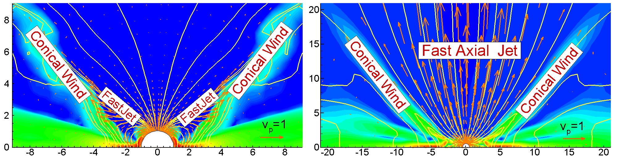
Figure 1: Two-component outflows observed in slowly (left) and rapidly (right) rotating magnetized stars for the reference runs described in this paper. The background shows the poloidal matter flux $F_{m}=\rho v_{p}$, the arrows are the poloidal velocity vectors, and the lines are sample magnetic field lines. The labels point to the main outflow components.

1 Introduction

Outflows or jets are observed from many disk accreting objects ranging from young stars to systems with white dwarfs, neutron stars, and black holes (e.g., Livio 1997).

A large body of observations exists for outflows from young stars at different stages of their evolution, ranging from protostars, where powerful collimated outflows are observed, to classical T Tauri stars (CTTSs), where the outflows are weaker and often less collimated (see review by Ray et al. 2007). Correlation between the disk and jet power had been found in many CTTSs (e.g., Cabrit et al. 1990; Hartigan, Edwards & Gandhour 1995). A significant number of CTTSs show signs of outflows in spectral lines, in particular in He I where two distinct components of outflows had been found (Edwards et al. 2003, 2006; Kwan, Edwards, & Fischer 2007). Outflows are also observed from accreting compact stars such as accreting white dwarfs in symbiotic binaries (e.g., Sokoloski & Kenyon 2003), or from the vicinity of neutron stars, such as from Circinus X-1 (Heinz et al. 2007).

Different theoretical models have been proposed to explain the outflows from protostars and CTTSs (see review by Ferreira, Dougados, & Cabrit 2006). The models include those where the outflow originates from a radially distributed disk wind (Königl & Pudritz 2000; Casse & Keppens 2004; Ferreira et al. 2006) or from the innermost region of the accretion disk (Lovelace, Berk & Contopoulos 1991). Further, there is the X-wind model (Shu et al. 1994; 2007; Najita & Shu 1994; Cai et al. 2008) where most of the outflow originates from the disk-magnetosphere boundary. The maximum velocities in the outflows are usually of the order of the Keplerian velocity of the inner region of the disk (or higher). This favors the models where the outflows originate from the inner disk region, or from the disk-magnetosphere boundary (if the star has a dynamically important magnetic field).

Outflows from the disk-magnetosphere boundary were investigated in early simulations by Hayashi, Shibata & Matsumoto (1996) and Miller & Stone (1997). A one-time episode of outflows from the inner disk and inflation of the innermost field lines connecting the star and the disk were observed for a few dynamical time-scales. Somewhat longer simulation runs were performed by Goodson et al. (1997, 1999), Hirose et al. (1997), Matt et al. (2002) and Küker, Henning & Rüdiger (2003) where several episodes of field inflation and outflows were observed. These simulations hinted at a possible long-term nature for the outflows. However, the simulations were not sufficiently long to establish the behavior of the outflows. Much longer simulation runs were obtained by treating the disk as a boundary condition (e.g. Fendt & Elsner 1999, 2000; Matsakos et al. 2008; Fendt 2009; see also von Rekowski & Brandenburg 2004; Yelenina, Ustyugova & Koldoba 2006). These simulations help understand, for example, the roles of the disk wind and stellar wind components in the outflow and collimation. However, for understanding the launching mechanisms it is important to have a realistic, low-temperature disk and to solve the full MHD equations in all of the disk and coronal space.

The goal of this work is to obtain long-lasting (robust) outflows from a realistic low-temperature disk (not a boundary condition) into a high-temperature, low-density corona. We obtained such outflows in two main cases: (1) when the star rotates slowly but the field lines are bunched up into an X-type configuration, and (2) when the star rotates rapidly, in the propeller regime (e.g., Illarionov & Sunyaev 1975; Alpar & Shaham 1985; Lovelace, Romanova & Bisnovatyi-Kogan 1999) and the condition for bunching is also satisfied. In both cases, two-component outflows have been observed (see Fig. 1). One component originates at the inner edge of the disk and has a narrow-shell conical shape, and therefore we call it a “conical wind”. The other component is a magnetically (or centrifugally) driven high-velocity low-density wind which flows along stellar field lines. We call it a “jet”. The jet may be very powerful in the propeller regime. Below we discuss both regimes in detail (see §3 -§4) after description of the numerical approach (see §2). In §5 we discuss different properties of outflows. In §6 we present exploratory 3D simulations of conical winds, and in §7 we compare conical winds and propeller outflows with the $X$-wind model. In §8 we apply the model to different types of stars, and in §9 we present our conclusions. Appendixes A and B clarify different aspects of the numerical model. Appendix C summarizes results of different runs for a variety of parameters.

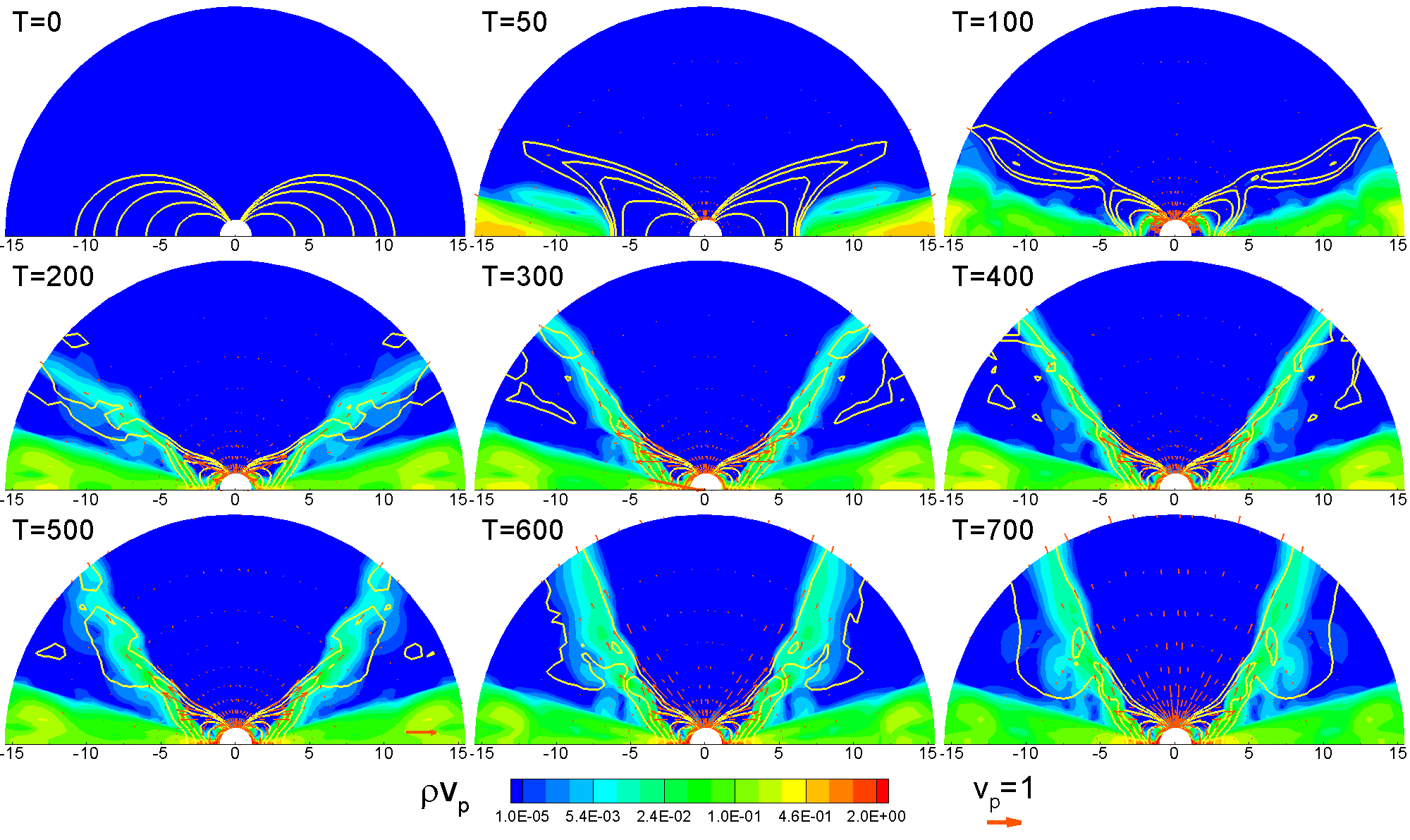
Figure 2: Conical winds at different times $T$. The background shows the poloidal matter flux $\rho v_{p}$ (with the scale below the plots), the arrows are the poloidal velocity vectors, and the lines are sample magnetic field lines (same set in all frames). Time $T$ is measured in Keplerian rotation periods at $r=1$. For example, for CTTS $T_{0}=1.04$ days (see Table 1) and time $T=700$ corresponds to 2 years. The sample vector $v_{p}=1$ corresponds to $v_{0}=195$ km/s.

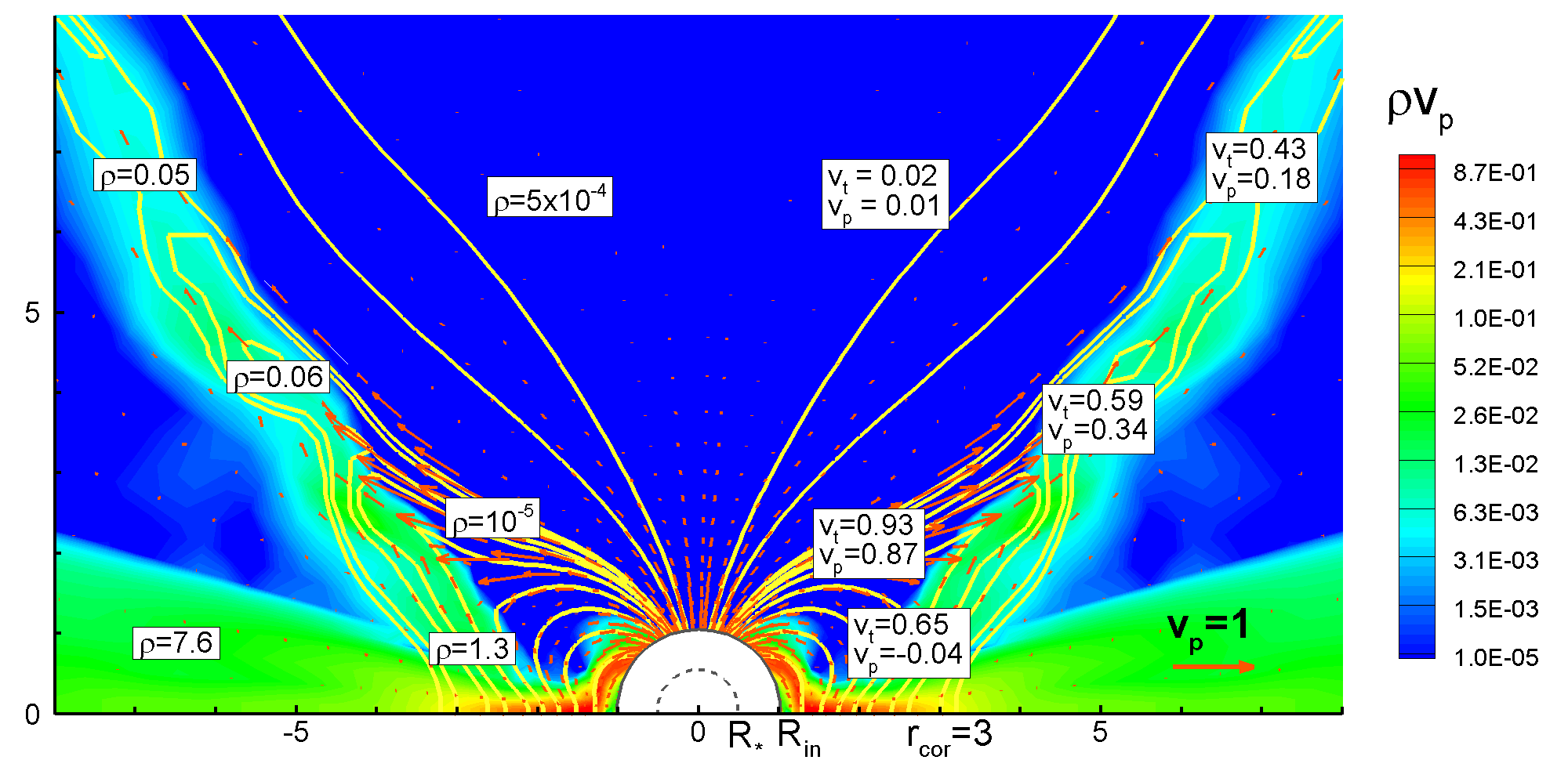
Figure 3: The poloidal matter flux $\rho v_{p}$ (with the scale on the right-hand side), sample magnetic field lines, and velocity vectors in the conical wind at time $T=500$. Sample numbers are given for the dimensionless poloidal $v_{p}$ and total $v_{t}$ velocities, and for the density $\rho$. To obtain the dimensional values one needs to multiply these numbers by the reference values given in the Table 1. For example, for application to CTTS: $v_{p}=1$ corresponds to $v_{0}=195$ km/s, $\rho=1$ corresponds to $\rho_{0}=4.1\times 10^{-13}$ g cm^-3, and the distance $r=1$ corresponds to $R_{0}=0.02$ AU.

2 Numerical Model

We simulate the outflows resulting from disk-magnetosphere interaction using the equations of axisymmetric MHD described below. Axisymmetric simulations of the outflows are similar to those performed earlier for the propeller regime (e.g., U06), but differ in initial and boundary conditions. Below we give an outline of the numerical model.

2.1 Basic Equations

Outside of the disk the flow is described by the equations of ideal MHD. Inside the disk the flow is described by the equations of viscous, resistive MHD. In an inertial reference frame the equations are:

$${\frac{\partial\rho}{\partial t}+{\bf\nabla}\cdot\left(\rho{\bf v}\right)}=0~{},$$ (1)

$${\frac{\partial(\rho{\bf v})}{\partial t}+{\bf\nabla}\cdot{\cal T}}=\rho~{}{\bf g}~{},$$ (2)

$${\frac{\partial{\bf B}}{\partial t}-{\bf\nabla}\times({\bf v}\times{\bf B})+{\bf\nabla}\times\left(\eta_{t}{\bf\nabla}\times{\bf B}\right)}=0~{},$$ (3)

$${\frac{\partial(\rho S)}{\partial t}+{\bf\nabla}\cdot(\rho S{\bf v})}=Q~{}.\$$ (4)

Here, $\rho$ is the density and $S$ is the specific entropy; $\bf v$ is the flow velocity; $\bf B$ is the magnetic field; $\cal{T}$ is the momentum flux-density tensor; $Q$ is the rate of change of entropy per unit volume; and ${\bf g}=-(GM/r^{2})\hat{{\bf r}}$ is the gravitational acceleration due to the star, which has mass $M$. The total mass of the disk is negligible compared to $M$. The plasma is considered to be an ideal gas with adiabatic index $\gamma=5/3$, and $S=\ln(p/\rho^{\gamma})$. We use spherical coordinates $(r,\theta,\phi)$ with $\theta$ measured from the symmetry axis. The condition for axisymmetry is $\partial/\partial\phi=0$. The equations in spherical coordinates are given in U06.

The stress tensor $\cal T$ and the treatment of viscosity and diffusivity are described in Appendix A. Briefly, both the viscosity and the magnetic diffusivity of the disk plasma are considered to be due to turbulent fluctuations of the velocity and the magnetic field. We adopt the standard hypothesis where the molecular transport coefficients are replaced by turbulent coefficients. To estimate the values of these coefficients, we use the $\alpha$-model of Shakura and Sunyaev (1973) where the coefficient of the turbulent kinematic viscosity $\nu_{t}=\alpha_{v}c_{s}^{2}/\Omega_{K}$, where $c_{s}$ is the isothermal sound speed and $\Omega_{K}(r)$ is the Keplerian angular velocity. Similarly, the coefficient of the turbulent magnetic diffusivity $\eta_{t}=\alpha_{d}c_{s}^{2}/\Omega_{K}$. Here, $\alpha_{v}$ and $\alpha_{d}$ are dimensionless coefficients which are treated as parameters of the model.

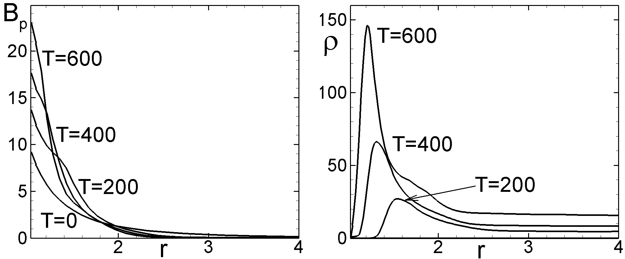
Figure 4: Left panel: equatorial distribution of the poloidal magnetic field in the inner part of the simulation region at different times $T$. Right panel: same as left panel but for density.

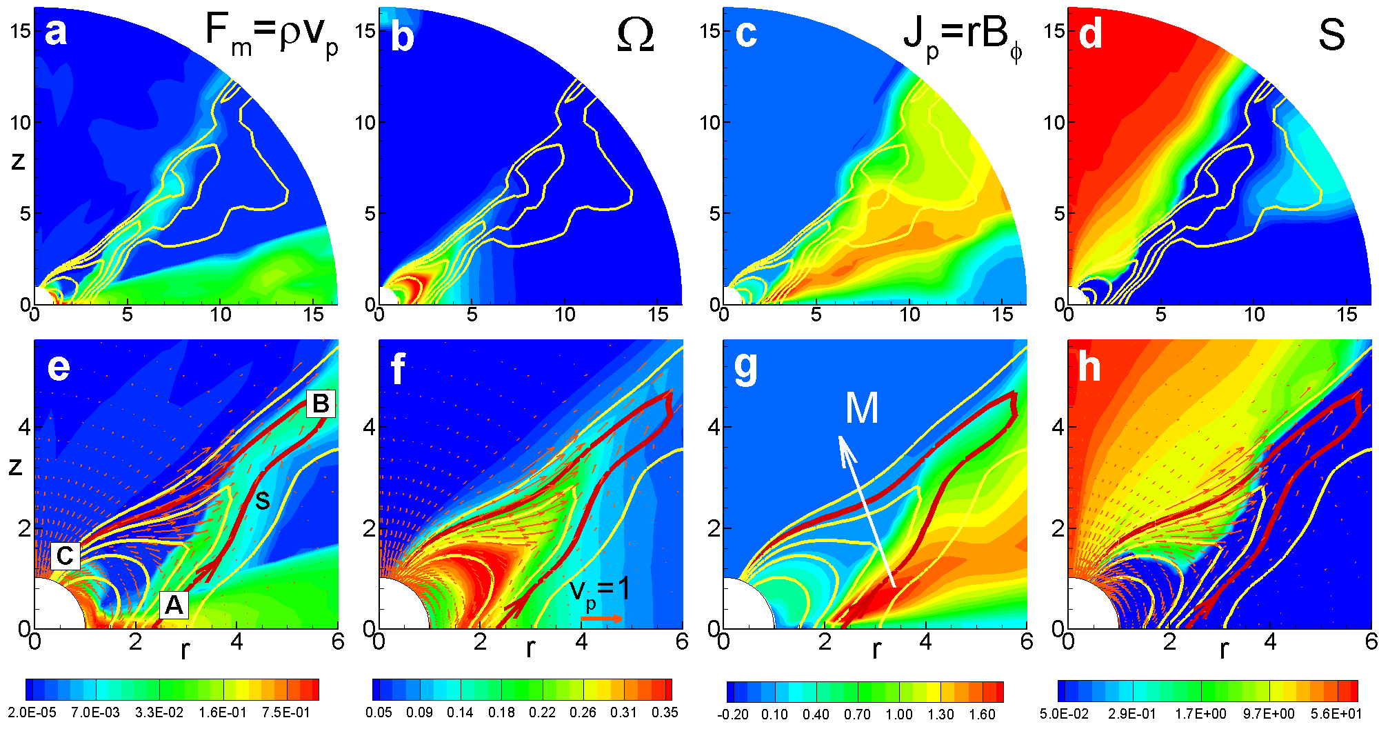
Figure 5: The background shows different parameters of a conical wind at time $T=500$, in the full simulation region, panels a-d, and near the star, panels e-h. The background shows (from left to right): the poloidal matter flux, $F_{m}=\rho v_{p}$, the angular velocity $\Omega$, the poloidal current $J_{p}=rB_{\phi}$, and the entropy $S$. Lines are sample magnetic field lines. Vectors are velocity vectors. The thick red line and the marks A, B, C show one of the field lines and positions along this line which are used for analysis of the forces and velocities in Fig. 6. The white vector in panel g shows schematically the direction of the magnetic force, M.

2.2 Reference Units

The MHD equations are solved in dimensionless form so that the results can be readily applied to different accreting stars (see §7). We take the reference mass $M_{0}$ to be the mass $M$ of the star. The reference radius is taken to be twice the radius of the star, $R_{0}=2R_{*}$. The surface magnetic field $B_{*}$ is different for different types of stars. The reference velocity is $v_{0}=(GM/R_{0})^{1/2}$. The reference time-scale $t_{0}=R_{0}/v_{0}$, and the reference angular velocity $\Omega_{0}=1/t_{0}$. We measure time in units of $P_{0}=2\pi t_{0}$ (which is the Keplerian rotation period at $r=R_{0}$). In the plots we use the dimensionless time $T=t/P_{0}$. The reference magnetic field is $B_{0}=B_{*}(R_{*}/R_{0})^{3}/{\tilde{\mu}}$, where $\tilde{\mu}$ is the dimensionless magnetic moment. The reference density is taken to be $\rho_{0}=B_{0}^{2}/v_{0}^{2}$. The reference pressure is $p_{0}=B_{0}^{2}$. The reference temperature is $T_{0}=p_{0}/{\cal R}\rho_{0}=v_{0}^{2}/{\cal R}$, where ${\cal R}$ is the gas constant. The reference accretion rate is $\dot{M}_{0}=\rho_{0}v_{0}R_{0}^{2}$. The reference energy flux is $\dot{E}_{0}=\dot{M}_{0}v_{0}^{2}$. The reference angular momentum flux is $\dot{L}_{0}=\dot{M}_{0}v_{0}R_{0}$.

The reference units are defined in such a way that the dimensionless MHD equations have the same form as the dimensional ones, equations (1)-(4) (for such dimensionalization we put $GM=1$ and ${\cal R}=1$). Table 1 shows examples of reference variables for different stars. We solve the MHD equations (1)-(4) using normalized variables: $\tilde{\rho}=\rho/\rho_{0}$, $\tilde{v}=v/v_{0}$, $\tilde{B}=B/B_{0}$, etc. Most of the plots show the normalized variables (with the tildes implicit). To obtain dimensional values one needs to multiply values from the plots by the corresponding reference values from Table 1.

	Protostars	CTTSs	Brown dwarfs	White dwarfs	Neutron stars
$M(M_{\odot})$	0.8	0.8	0.056	1	1.4
$R_{*}$	$2R_{\odot}$	$2R_{\odot}$	$0.1R_{\odot}$	5000 km	10 km
$R_{0}$ (cm)	$2.8\times 10^{11}$	$2.8\times 10^{11}$	$1.4\times 10^{10}$	$1.0\times 10^{9}$	$2\times 10^{6}$
$v_{0}$ (cm s-1)	$1.95\times 10^{7}$	$1.95\times 10^{7}$	$1.6\times 10^{7}$	$3.6\times 10^{8}$	$9.7\times 10^{9}$
$P_{*}$	$1.04$ days	$5.6$ days	$0.13$ days	$89$ s	$6.7$ ms
$P_{0}$	$1.04$ days	$1.04$ days	$0.05$ days	$17.2$ s	$1.3$ ms
$B_{*}$ (G)	$3.0\times 10^{3}$	$10^{3}$	$2.0\times 10^{3}$	$10^{6}$	$10^{9}$
$B_{0}$ (G)	37.5	12.5	25.0	$1.2\times 10^{4}$	$1.2\times 10^{7}$
$\rho_{0}$ (g cm-3)	$3.7\times 10^{-12}$	$4.1\times 10^{-13}$	$1.4\times 10^{-12}$	$1.2\times 10^{-9}$	$1.7\times 10^{-6}$
$n_{0}$ (1/cm-3)	$2.2\times 10^{12}$	$2.4\times 10^{11}$	$8.5\times 10^{11}$	$7.0\times 10^{14}$	$1.0\times 10^{18}$
$\dot{M}_{0}$($M_{\odot}$yr-1)	$1.8\times 10^{-7}$	$2.0\times 10^{-8}$	$1.8\times 10^{-10}$	$1.3\times 10^{-8}$	$2.0\times 10^{-9}$
$\dot{E}_{0}$ (erg s-1)	$2.1\times 10^{33}$	$2.4\times 10^{32}$	$2.5\times 10^{30}$	$5.7\times 10^{34}$	$6.0\times 10^{36}$
$\dot{L}_{0}$ (erg s-1)	$3.1\times 10^{37}$	$3.4\times 10^{36}$	$1.7\times 10^{33}$	$1.6\times 10^{35}$	$1.2\times 10^{33}$
$T_{d}$ (K)	$2293$	$4586$	$5274$	$1.6\times 10^{6}$	$1.1\times 10^{9}$
$T_{c}$ (K)	$2.3\times 10^{6}$	$4.6\times 10^{6}$	$5.3\times 10^{6}$	$8.0\times 10^{8}$	$5.6\times 10^{11}$

Table 1: Reference values for different types of stars. We choose the mass $M$, radius $R_{*}$, equatorial magnetic field $B_{*}$ and the period $P_{*}$ of the star and derive the other reference values (see §2.2). To apply the simulation results to a particular star one needs to multiply the dimensionless values from the plots by the reference values from this table.

2.3 Initial and Boundary Conditions

We assume that the poloidal magnetic field of the star is an aligned dipole field ${\bf B}=[3({\hbox{\tenbg\char 22\relax}}\cdot{\bf r}){\bf r}-{\hbox{\tenbg\char 22\relax}}{r}^{2}]/r^{5},~{}$ where ¯ is the star’s magnetic moment. The initial density and temperature distributions are different in cases of conical winds and propeller-driven winds.

2.3.1 Conical Winds

Initial Conditions. At time $T=0$ the simulation region is filled with a low-density, high-temperature, isothermal plasma referred to as the corona. Initially it is non-rotating. Thus the density and pressure distributions in the corona are:

$$\rho=\rho_{c}\exp[GM/({\cal R}T_{c}r)],~{}~{}~{}p=p_{c}\exp[GM/({\cal R}T_{c}r)]~{},$$

where $T_{c}$ is the corona temperature, $\rho_{c}$ is the coronal density at the external boundary, $p_{c}=\rho_{c}{\cal R}T_{c}$.

We divide the external boundary $R_{out}$ into a disk region, $\theta_{d}<\theta<\pi/2$, and a corona region, $0<\theta<\theta_{d}$, with $\theta_{d}\approx 65^{\circ}$. Initially, there is no disk in the simulation region. When the simulations start, we permit high-density low-temperature matter to enter the simulation region through the disk boundary region, $\theta>\theta_{d}$, with a fixed density $\rho=\rho_{d}$. Matter continues to flow inward due to viscosity (see Appendix A). We increase the spin of the star gradually from a small value corresponding to $r_{cor}=R_{out}$ (where $r_{cor}=(GM/\Omega^{2})^{1/3}$) up to a final value $\Omega_{*}$. Information about the stellar rotation propagates rapidly (at the Alfvén speed) into the low-density corona.

We did simulations for a variety of parameters. However, we take one case with typical parameters to be our reference case and show the results for this case. In the reference case, the dipole moment of the star $\mu=10$; the density in the corona $\rho_{c}=0.001$, the density in the disk $\rho_{d}=10$; the corona is hot with temperature $T_{c}=1$; the disk is cold with temperature $T_{d}=(\rho_{c}/\rho_{d})T_{c}=10^{-4}$. The angular velocity of the star corresponds to a corotation radius $r_{cor}=3$, $\Omega_{*}=(GM/r_{cor}^{3})=0.19$. The coefficients of viscosity and diffusivity are $\alpha_{v}=0.3$ and $\alpha_{d}=0.1$. The dependences of our results on different parameters are discussed in Appendix C.

The boundary conditions at the inner boundary $r=R_{in}$ are the following: The frozen-in condition is applied to the poloidal component $\bf{B}_{p}$ of the field, such that $B_{r}$ is fixed while $B_{\theta}$ and $B_{\phi}$ obey “free” boundary conditions, $\partial B_{\theta}/\partial r=0$ and $\partial B_{\phi}/\partial r=0$. The density, pressure, and entropy also have free boundary conditions, $\partial(...)/\partial r=0$. The velocity components are calculated using free boundary conditions. Then, the velocity vector is adjusted to be parallel to the magnetic field vector in the coordinate system rotating with a star. Matter always flows inward at the star’s surface. Outflow to a stellar wind is not considered in this work.

The boundary conditions at the external boundary $r=R_{out}$ in the coronal region $0<\theta<\theta_{d}$ are free for all hydrodynamic variables. However, we prevent matter from flowing into the simulation region from this part of the boundary. We solve the transport equation for the flux function $\Psi$ so that the magnetic flux flows out of the region together with matter. If the matter has a tendency to flow back in, then we fix $\Psi$. In the disk region, $\theta_{d}<\theta<\pi/2$, we fix the density at $\rho=\rho_{d}$, and establish a slightly sub-Keplerian velocity, $\Omega_{d}=\kappa\Omega(r_{d})$, where $\kappa=1-0.003$ so that matter flows into the simulation region through the boundary. The inflowing matter has a fixed magnetic flux which is very small because $R_{out}\gg R_{in}$.

The boundary conditions on the equatorial plane and on the rotation axis are symmetric and antisymmetric.

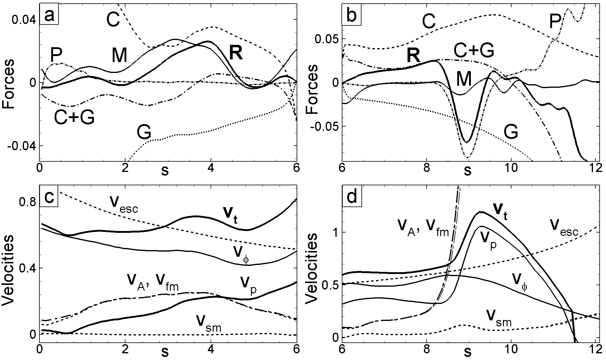
Figure 6: Panel a shows the projection of forces onto part AB of the bold field line shown in Fig. 5e. The labels are: $G-$gravitational, $C-$centrifugal, $M-$magnetic, $P-$pressure gradient, and $R-$sum of all forces. Panel b shows the projection of forces onto part BC of the field line. Panel c shows velocities along part AB of the field line: $v_{p}-$poloidal velocity, $v_{\phi}-$azimuthal velocity, $v_{t}-$total velocity, $v_{A}-$Alfvén speed, $v_{sm}-$slow-magnetosonic speed, $v_{fm}-$fast- magnetosonic speed, and $v_{esc}-$escape velocity. Panel d shows velocities along part BC of the field line.

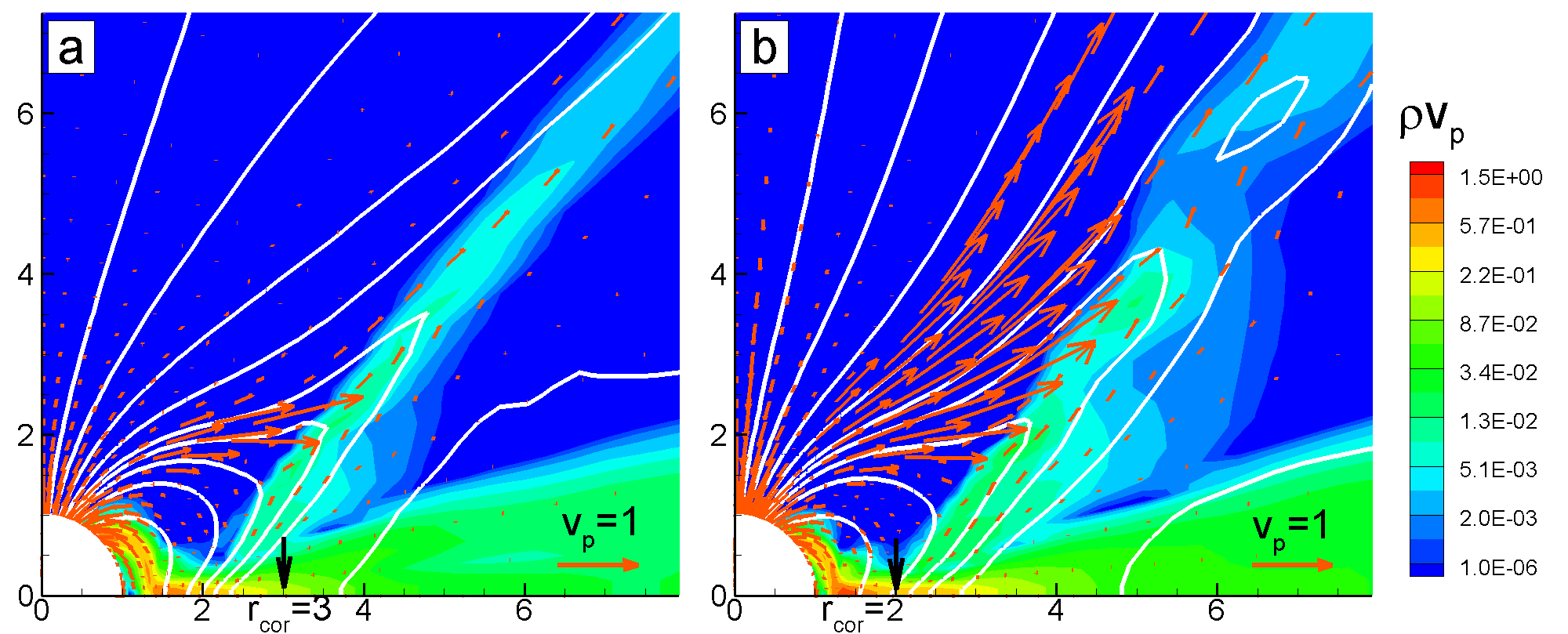
Figure 7: Panel a: Two components of outflow in the reference case ($r_{cor}=3$). Panel b: Same but for a more rapidly rotating star ($r_{cor}=2$). Both cases are shown at time $T=250$.

2.3.2 Propeller Regime

The initial and boundary conditions for the propeller regime are the same as those used in R05 and U06. Here, we summarize these conditions.

Initial Conditions. We place both the disk and the corona into the simulation region. We assume that the initial flow is barotropic with $\rho=\rho(p)$, and that there is no pressure jump at the boundary between the disk and corona. Then the initial density distribution (in dimensionless units) is the following:

$$\rho(p)=\left\{\begin{array}[]{lcl}p/{\cal R}T_{d}~{},~{}~{}~{}p>p_{b}~{}~{}~{}~{}{\rm and}~{}~{}~{}~{}r\sin\theta\geq r_{b}~{},\\[8.5359pt] p/{\cal R}T_{c}~{},~{}~{}~{}~{}p<p_{b}~{}~{}~{}~{}{\rm or}~{}~{}~{}~{}~{}~{}r\sin\theta\leq r_{b}~{},\end{array}\right.$$

where $p_{b}$ is the pressure on the surface which separates the cold matter of the disk from the hot matter of the corona. On this surface the density jumps from $p_{b}/T_{d}$ to $p_{b}/T_{c}$. Here $r_{b}$ is the inner disk radius. Because the density distribution is barotropic, the angular velocity is constant on coaxial cylindrical surfaces about the $z-$axis. Consequently, the pressure distribution may be determined from the Bernoulli equation,

$$F(p)+\Phi+\Phi_{c}=E={\rm const}~{}.$$

Here, $\Phi=-GM/|{\bf r}|$ is gravitational potential, $\Phi_{c}=\int_{r\sin\theta}^{\infty}\Omega^{2}(\xi)\xi d\xi$ is centrifugal potential, which depends only on the cylindrical radius $r\sin\theta$, and

$$F(p)=\left\{\begin{array}[]{lcl}{\cal R}T_{d}\ln(p/p_{b})~{},~{}~{}~{}p>p_{b}~{}~{}~{}~{}{\rm and}~{}~{}~{}r\sin\theta>r_{b}~{},\\[8.5359pt] {\cal R}T_{c}\ln(p/p_{b})~{},~{}~{}~{}~{}p<p_{b}~{}~{}~{}~{}{\rm or}~{}~{}~{}~{}r\sin\theta<r_{b}~{}.\end{array}\right.$$

The angular velocity of the disk is slightly sub-Keplerian, $\Omega(\theta=\pi/2)=\kappa\Omega_{K}$ ($\kappa=1-0.003$), due to which the density and pressure decrease towards the periphery. Inside the cylinder $r\leq r_{b}$ the matter rotates rigidly with angular velocity $\Omega(r_{b})=\kappa(GM/r_{b}^{3})^{1/2}$. For a gradual start-up we change the angular velocity of the star from its initial value $\Omega(r_{b})=5^{-3/2}\approx 0.09$ ($r_{b}=5$) to a final value of $\Omega_{*}=1$ over the course of three Keplerian rotation periods at $r=1$.

For the propeller regime we use a slightly different set of parameters compared with the conical wind case (in order to be consistent with our earlier simulations in R05, U06). Below we describe the similarities and differences: the dipole moment of the star is the same, $\mu=10$. The angular velocity of the star in the propeller regime is larger, $\Omega_{*}=1$. The initial density in the disk (at the inner edge) is $\rho_{d}=1$, which is smaller than the external density ($\rho_{d}=10$) in conical winds. The initial temperatures are a factor of two smaller than in conical winds, $T_{c}=(p/{\cal R}\rho)_{c}=0.5$, $T_{d}=0.0005$.

Boundary conditions for the propeller regime are similar to those for conical winds with the following differences. At the external boundary (disk region) we take free conditions for all variables. There is no condition of fixed density at the disk part of the boundary.

The system of MHD equations (1-4) was integrated numerically using the Godunov-type numerical scheme (see Appendix B). The simulations were done in the region $R_{in}\leq r\leq R_{out}$, $0\leq\theta\leq\pi/2$. The grid is uniform in the $\theta$-direction. The size steps in the radial direction were chosen so that the poloidal-plane cells were curvilinear rectangles with approximately equal sides. A typical region for investigation of conical winds was $1\leq r\leq 16$, with grid resolution $N_{r}\times N_{\theta}=51\times 31$ cells. A typical region for investigation of the propeller regime was $1\leq r\leq 48$ with grid resolution $N_{r}\times N_{\theta}=85\times 31$ cells. Test simulations at angular grids $N_{\theta}=51$ and $N_{\theta}=71$ were also performed. Each simulation run at the lowest resolution takes about two months of computing time on a single processor. We performed $40$ different simulation runs for different parameters on our local cluster of $20$ computers for the investigation of conical winds. 3D simulation runs were performed with “Cubed sphere” parallel code on NASA high-performance facilities.

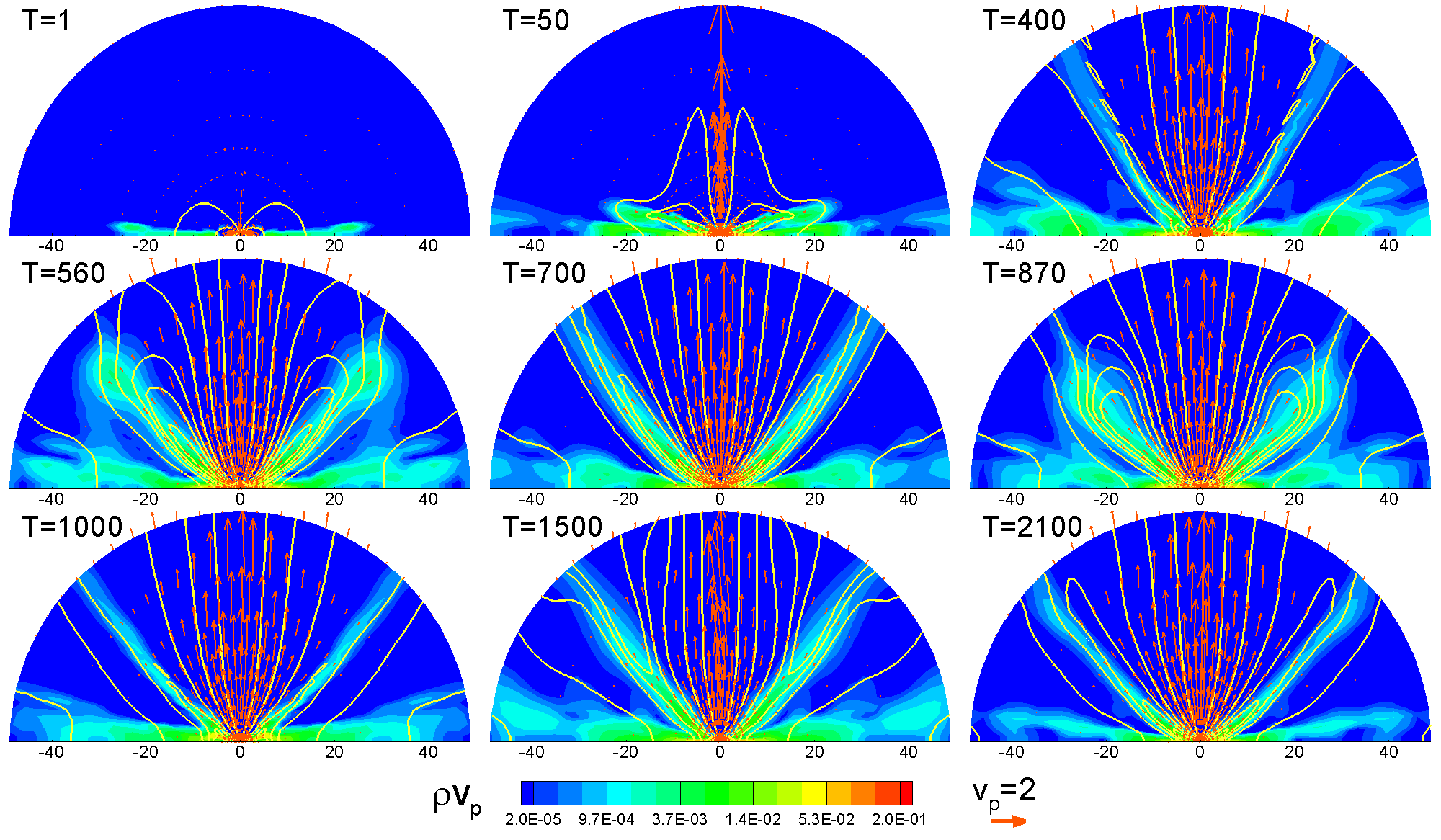
Figure 8: Same as in Fig. 2 but for the propeller regime. The simulation time $T=2200$ corresponds to 6 years. The sample vector $v_{p}=2$ corresponds to $v=2\times v_{0}=390$ km/s.

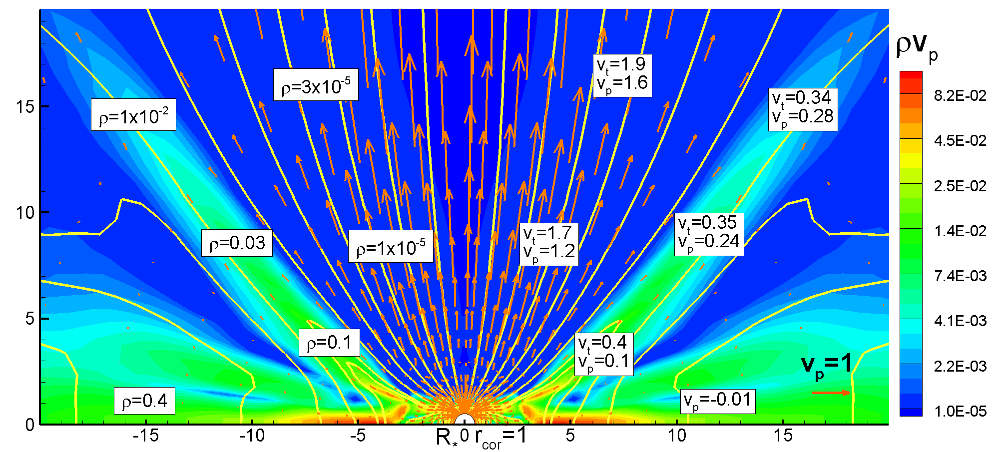
Figure 9: Same as in Fig. 3 but for the propeller regime at time $T=1400$.

3 Matter flow in conical winds and in the propeller regime

3.1 Matter flow, velocities, and forces in conical winds

A large number of simulations were done in order to understand the origin and nature of conical winds. All of the key parameters were varied in order to ensure that there is no special dependence on any parameter (see Appendix C). We observed that the formation of conical winds is a common phenomenon for a wide range of parameters. They are most persistent and strong in cases where the viscosity and diffusivity coefficients are not very small, $\alpha_{v}\gtrsim 0.03$, $\alpha_{d}\gtrsim 0.03$. Another important condition is that $\alpha_{v}\gtrsim\alpha_{d}$; that is, the magnetic Prandtl number of the turbulence, Pr${}_{m}=\alpha_{v}/\alpha_{d}\gtrsim 1$. This condition favors the bunching of the stellar magnetic field by the accretion flow.

For a discussion of the physics of conical winds we focus on one set of parameters which serves as a reference case. These parameters are: $\alpha_{v}=0.3$ and $\alpha_{d}=0.1$; $\Omega_{*}=0.19$ ($r_{cor}=3$), $\mu=10$, $\rho_{d}=10$, and $\rho_{c}=10^{-3}$, $T_{c}=1$, $T_{d}=10^{-4}$. The simulations were done in dimensionless form and can be applied to different stars (see Table 1). However, for illustration we often show dimensional examples for CTTSs with parameters taken from Table 1. For example, in application to CTTSs, $\Omega_{*}=0.19$ corresponds to $P_{*}=5.4$ days and the unit of time used in the figures is $P_{0}=1.04$ days (see Table 1 for other reference values).

Fig. 2 shows snapshots of simulations at different times $T$. One can see that the cold dense disk matter enters the simulation region from the external boundary and moves inward towards the star on the viscous time-scale. The accretion flow bunches up the field lines of the dipole field to a relatively small region near the star. All field lines shown at $T=0$ are bunched up close to the star by $T=100$. The inclined configuration of the resulting poloidal field and inflation of external field lines create conditions favorable for matter outflow from the inner disk. The outflow starts at $T\sim 120$ and gets stronger later. Matter flows from the inner disk into hollow, conical shaped winds with half-opening angle $\theta\sim 30^{\circ}-40^{\circ}$. The conical winds are non-stationary, showing variations associated with events of inflation and reconnection of the magnetic field lines (see animations at http://www.astro.cornell.edu/$\sim$romanova/conical.htm). The simulation runs continue for a long time, about $T=740$, which is about 2 years for CTTSs. The outflows remain strong until the end of the simulation runs. It is reasonable to conclude that these accretion-driven outflows into the conical winds will persist as long as matter is supplied from the disk.

Fig. 3 shows the configuration at $T=500$. One can see that the disk matter comes close to the star and accretes onto the star through a small dense funnel. Some field lines are strongly inflated, and the conical wind flows from the disk along these lines. There is also a set of partially inflated field lines (a dead zone) where accretion does not occur (e.g., Ostriker & Shu 2005; Spruit & Taam 1990). Matter in conical winds rotates with the Keplerian velocity at the base of outflow, $v_{\phi}\approx v_{K}$. It continues to rotate rapidly in the conical wind at larger distances from the star. The poloidal velocity $v_{p}$ increases gradually from very small values at the beginning of the outflow, up to $v_{p}\approx 0.5v_{K}$. The main contribution to the total velocity $v_{t}$ comes from the azimuthal component. There is another, high-velocity component of the low-density matter which flows along the stellar field lines. In application to CTTSs the velocity is $>200$ km/s.

Fig. 4 shows the variation of the density and the poloidal magnetic field along the equator in the inner part of the simulation region at different times $T$. One can see that the disk matter has approximately constant density at different radii, but there is a density peak closer to the star. The peak increases with time, but it does not appreciably influence the fluxes calculated at the surface of the star (see Fig. 14). Fig. 4 also shows that the poloidal magnetic field of the star is compressed, and the compression increases with time. Compression of the star’s magnetic field by the accretion flow is also assumed in the X-wind model (e.g., Najita & Shu 1994).

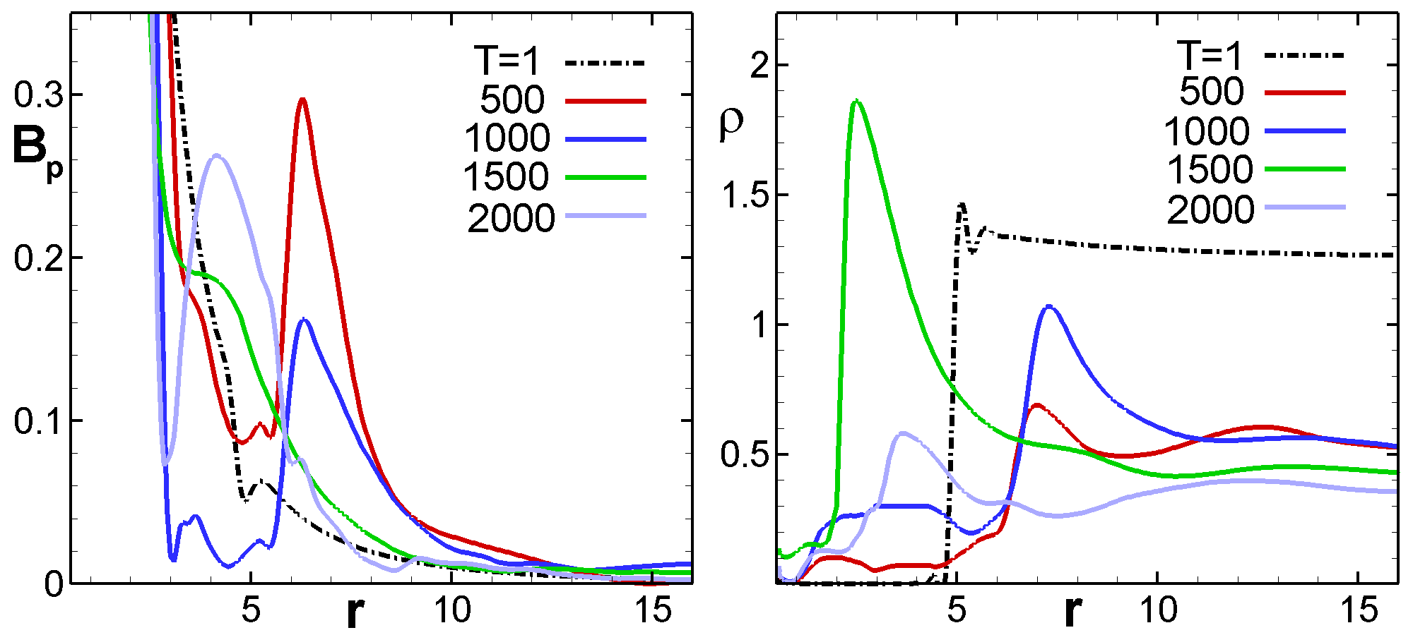
Figure 10: Same as in Fig. 4 but in the propeller regime.

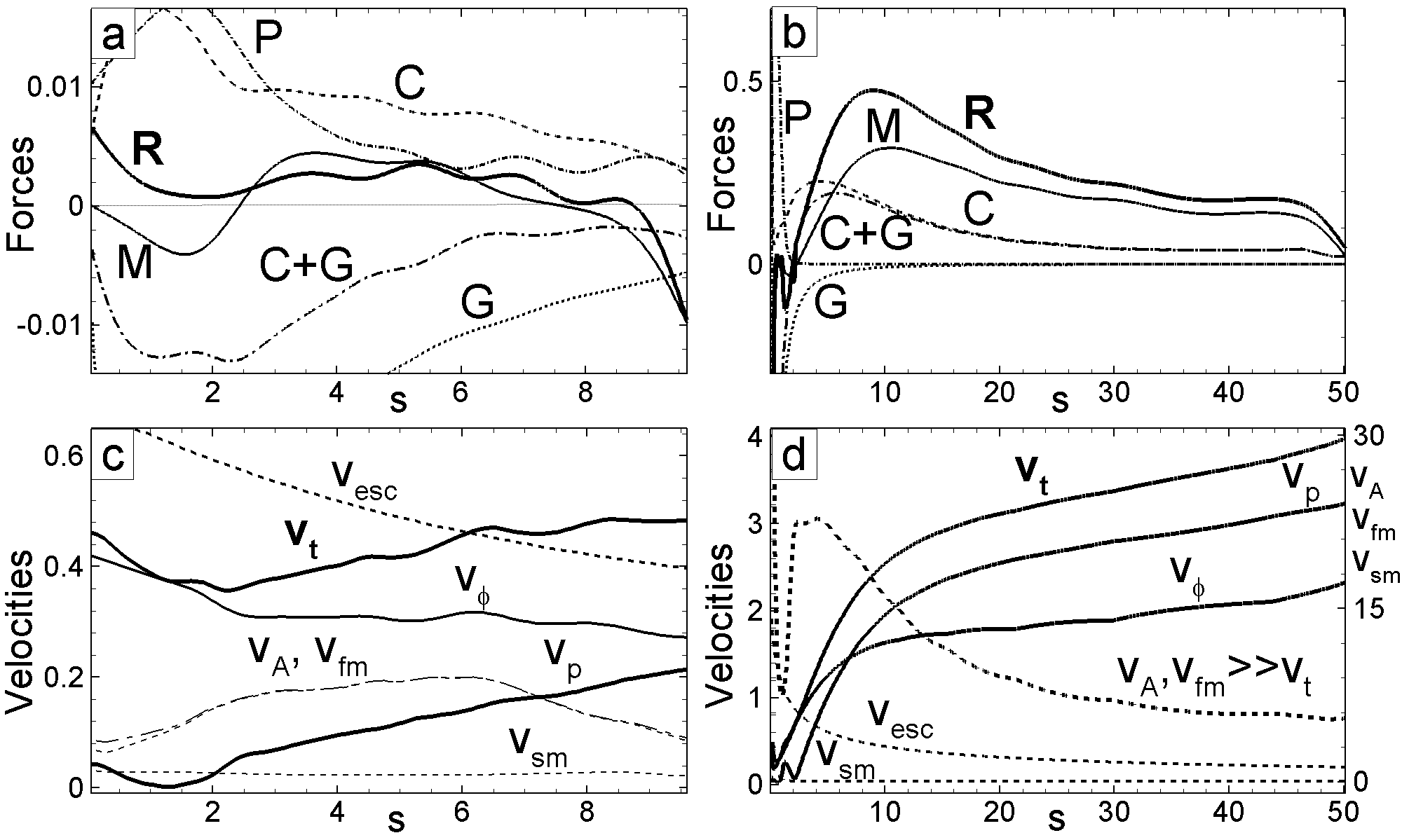
Figure 11: Forces (top panels) and velocities (bottom panels) along the field lines in the propeller regime at $T=1400$. Left panels: forces and velocities along the closed magnetic field line which starts in the disk (at $r=4.3$) and ends on the star. We take only the part of the line up to the neutral point where the line curves towards the star($B_{r}=0$). Forces are projected onto the field line. Labels are the same as in Fig. 6. Right panels: forces and velocities along the open field line which starts on the surface of the star. Note that the scale for $v_{A}$, $v_{\rm sm}$, $v_{\rm fm}$ is different from that for other velocities.

To understand the physics of conical winds in greater detail we show in Fig. 5 the distribution of different parameters at time $T=500$. Panels b and f show that the innermost region of the closed magnetosphere rotates with the angular velocity of the star ($1.2\leq r\leq 1.8$). At larger distances ($r>2.5$), the corona above the disk rotates with the angular velocity of the disk. Strongly inclined field lines which start in the disk go through regions of lower and lower angular velocity and are strongly wound up owing to the difference in the angular rotation rates along the lines. This leads to a strong poloidal current flow $J_{p}\propto rB_{\phi}$ above the disk (see panels c and g) which gives rise to the magnetic force $F_{p}\sim-{\bf\nabla}[(rB_{\phi})^{2}]$. This is the main force driving matter into the conical wind. Driving of winds by the magnetic force from the inner disk was proposed earlier by Lovelace et al. (1991). The direction of the magnetic force is shown schematically in Fig. 5g. It acts upwards and towards the axis, which is different from the centrifugal force. This determines three of the important properties of conical winds: (1) their small opening angle; (2) the fact that the wall of the cone is narrow, and (3). the gradual collimation of conical winds. If the centrifugal force were dominate (e.g. Blandford & Payne 1982) then the cone would have a wider opening angle and outflow would flow over a wide range of directions (as in the X-wind model of Shu et al. 1994). Panels d and h show the distribution of entropy $S$ which shows that matter flowing from the disk into the wind is cold and it is not thermally driven. To analyze the forces driving matter into the conical winds we select one of the field lines, $s$, (see red bold line in panels e-h) and we project forces onto this field line. We split the line into two parts (see panel a). Part ${\bf AB}$ starts from the disk and ends at the place where the line curves towards the star; part BC continues from there to the surface of the star .

Fig. 6a shows the projection of all forces onto part AB of the field line. One can see that the main force accelerating matter into the conical wind is the magnetic force $M$. The centrifugal ($C$) and gravitational ($G$) forces approximately compensate each other and the sum $C+G$ is negative. The pressure gradient force $P$ is small. The $\theta$-component of the magnetic force leads to frequent forced reconnection events of the inflated field lines and to ejection of plasmoids into the conical wind. Panel b shows the projection of the forces onto segment BC of the field line. One can see that it is chiefly the centrifugal force which accelerates the low-density matter to high velocities in this region. Panel c shows that in the conical wind the poloidal velocity $v_{p}$ (along part ${\bf AB}$) gradually increases and crosses the slow magnetosonic ($v=v_{sm}$), Alfvén ($v=v_{A}$) and fast magnetosonic ($v=v_{fm}$) surfaces. Matter rotates rapidly, therefore the azimuthal component $v_{\phi}$ is much larger than poloidal one, and the total velocity $v_{t}$ is determined by the azimuthal rotation of the flow. Panel d shows that there is an interval of high velocity along the stellar part (BC) of the field line. Thus, we observe a two-component flow: (1) a high-density low-velocity conical wind which is the main component of the outflows, and (2) a low-density fast outflow along the stellar field lines which occupies a much smaller region.

We find that the region of the fast coronal flow increases in size with the star’s rotation rate. As an example we decreased the corotation radius from $r_{cor}=3$ ($\Omega_{*}=0.19$) to $r_{cor}=2$ ($\Omega_{*}=0.35$) and observed that the region of fast coronal flow increased significantly. Fig. 7 shows the difference. The region is even larger for smaller corotation radii when the star is closer to the propeller regime. In the propeller regime (see §4) the fast jet component occupies the entire region within the conical wind and is very powerful. The star spins up for both $R_{cor}=2$ and $3$. Cases $R_{cor}=1,1.5$ correspond to the propeller regime where the star spins down due to the interaction with the disk and corona. We did not perform a refined search for the rotational equilibrium state, in which the star has alternate spin-up and spin-down periods, but zero torque on an average (e.g. R02, Long et al. 2005). In this state we expect the jet component to occupy a large part of the region above conical winds. Even a weak stellar wind (not considered in this paper) may enhance the jet component.

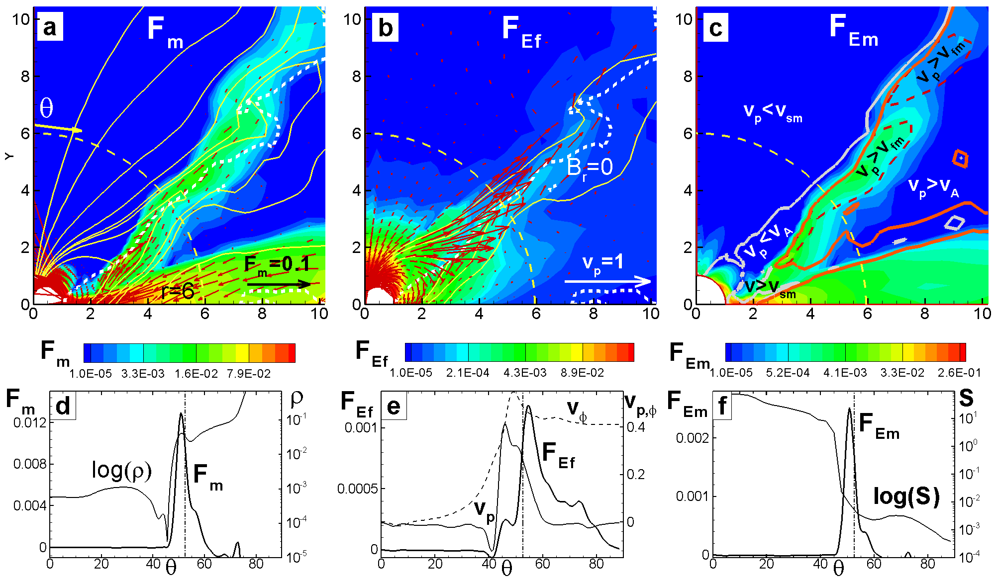
Figure 12: Top panels: matter and energy fluxes at $T=500$. Bottom panels: angular distribution of different quantities at radius $r=6$ (starting from the axis). Panel a: the background and vectors show matter flux $F_{m}$, lines are poloidal field lines. The thick dashed line shows the neutral line of the magnetic flux where $B_{r}=0$. Panel b: the background shows the energy flux carried by the magnetic field, $F_{\rm Ef}$, vectors are poloidal velocity vectors. Panel c: the background shows the energy flux carried by the matter, $F_{\rm Ef}$. The solid red line is the line where $v_{p}=v_{A}$, red dashed line corresponds to $v_{p}=v_{\rm fm}$, the solid white line corresponds to $v_{p}=v_{\rm sm}$. Panel d: distribution of density $\rho$ and matter flux $F_{m}$ at $r=6$; Panel e: same but for $F_{\rm Ef}$ and velocities $v_{p}$, $v_{\phi}$; Panel f: same but for $F_{\rm Em}$ and entropy S. Dashed vertical line shows position of the neutral point, $B_{r}=0$.

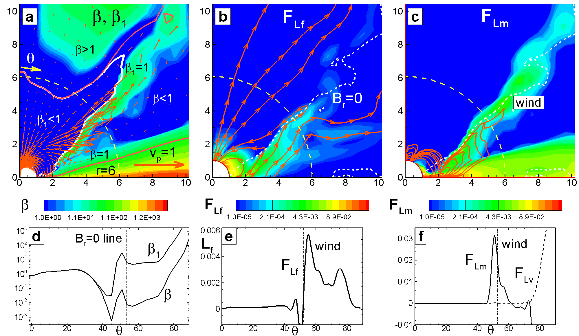
Figure 13: The figure is similar to Fig. 12, but different quantities are shown. Panel a: the background shows the distribution of the kinetic beta parameter $\beta_{1}$. The solid white line is $\beta_{1}=1$ line, the red line is $\beta=1$ line. Arrows are velocity vectors. Panel b: the background shows angular momentum flux carried by the magnetic field, $F_{\rm Lf}$, streamlines show direction of this flux; the thick dashed line corresponds to $B_{r}=0$. Panel c: the background shows angular momentum flux carried by the matter, $F_{\rm Lm}$. The solid red lines show contours of the $F_{\rm Lf}$ flux; Panel d: angular distribution of $\beta$ and $\beta_{1}$ at $r=6$. The dashed vertical line shows the position of the neutral line $B_{r}=0$. Panel e: same but for $F_{\rm Lf}$. Panel f: same but for $F_{\rm Lm}$ and the viscous flux $F_{\rm Lv}$ (dashed line).

3.2 Matter flow, velocities and forces in the propeller regime

Here we consider outflows from rapidly rotating stars in the propeller regime. In earlier work we performed multiple simulation runs of the propeller stage at a wide variety of parameters (R05; U06). Here we take the reference run shown in R05 and perform additional analysis. The parameters are $P_{*}=1$ day, $\alpha_{v}=0.3$ and $\alpha_{d}=0.2$ (see §2.3.2 for the other parameter values).

Fig. 8 shows snapshots of the matter flow in the propeller regime at different times $T$. One can see that the outflow appears at $T\approx 50$ and continues for a long time ($T=2200$ rotations, or about 6 years in application to protostars). These simulations are about $10$ times longer than previous simulations of outflows from a real disk (e.g. Goodson et al. 1997; Matt et al. 2002; Küker et al. 2003). They are comparable in length with simulations of outflows from the disk as a boundary condition (e.g., Fendt 2009), although here we consider outflows form the “real” cold disk to a hot low-density corona.

Fig. 8 also shows that the outflow has two components. One is a conical-shaped wind similar to the conical winds of slowly rotating stars discussed earlier. The other component is a fast flow of matter interior to the conical winds, which we term the axial jet. The disk-magnetosphere interaction is strongly non-stationary; the magnetic field lines episodically inflate and the disk oscillates. The conical wind component seems to be weakly collimated inside the simulation region. The jet component has stronger collimation. The jet collimation is stronger in the flow closer to the axis, and is enhanced during periods of strong inflation, like at times $T=560$ and $870$. See animations of propeller-driven outflows at http://www.astro.cornell.edu/$\sim$romanova/propeller.htm.

Fig. 9 shows a typical snapshot from our simulations at time $T=1400$, with the dimensionless density and velocity at sample points (see Table 1 for reference values). One can see that the velocities in the conical wind component are similar to those in conical winds around slowly rotating stars. Matter launched from the disk has a velocity that is mainly azimuthal and approximately Keplerian. It is gradually accelerated to poloidal velocities $v_{p}\sim(0.3-0.5)v_{K}$. The flow has a high density and carries most of the disk mass into the outflows. The situation is the opposite in the axial jet component: the density is $10^{2}-10^{3}$ times lower, while the poloidal and total velocities are much higher. Thus we find a two-component outflow: a dense, slow conical wind and a low-density, fast axial jet.

Fig. 10 shows the time-variation of the equatorial density and the poloidal magnetic field in the inner part of the simulation region. One can see that the density and the poloidal magnetic field are strongly enhanced at the inner edge of the disk, and the inner disk radius shows large oscillation (see also R05, U06).

Fig. 11a shows the projection of different forces onto a closed field line which starts in the disk at $r=4.3$ where the base of the conical wind (see Fig. 9). We take only the part of the line from the disk to the neutral point where $B_{r}=0$ (this is the analog of part AB of the line in Fig. 5e). One can see that the forces are large but more or less compensate each other. The magnetic force ($M$) seems to drive matter from the disk into the conical wind, though other forces, such as the centrifugal ($C$) and pressure gradient ($P$) forces are also important. It is interesting that conical winds in slowly rotating stars and in stars in the propeller regime are similar, but that the distribution of forces is somewhat different. In conical winds the winding of the field lines gives rise to a magnetic force in one localized region (above the inner disk) and this force dominates. In the propeller regime the disk oscillates strongly, and it is important that the magnetosphere presents a centrifugal barrier for this matter, and therefore the centrifugal and pressure gradient forces have a larger role. The magnetic force remains important.

Panel b shows the forces along the coronal field line which starts on the surface of the star. We consider the second line from the axis in Fig. 9, which is strongly inflated and is a representative line for the description of matter flow into the axial jet. One can see that the magnetic force $M$ is much larger than the other forces and is the main force accelerating matter into the jet.

Panel c shows velocities along the disk field line (as in panel a). One can see that the azimuthal component $v_{\phi}$ dominates, while the poloidal velocity $v_{p}$ increases gradually from a very small value near the disk up to values comparable with $v_{\phi}$. It crosses the slow magnetosonic surface just above the disk, and later, the Alfvén and the fast magnetosonic surfaces.

Panel d shows that in the coronal region, the velocities are high and the poloidal velocity dominates. Matter crosses the slow magnetosonic surface but stays sub-Alfvénic. Both the Alfvén, $v_{A}$, and the fast magnetosonic, $v_{\rm fm}$, velocities are about $10$ times larger than the flow velocity in the axial jet (note the scale at the right-hand side). The flow is in the Poynting flux regime found in simulations by Ustyugova et al. (2000) and analyzed theoretically by Lovelace et al. (2002).

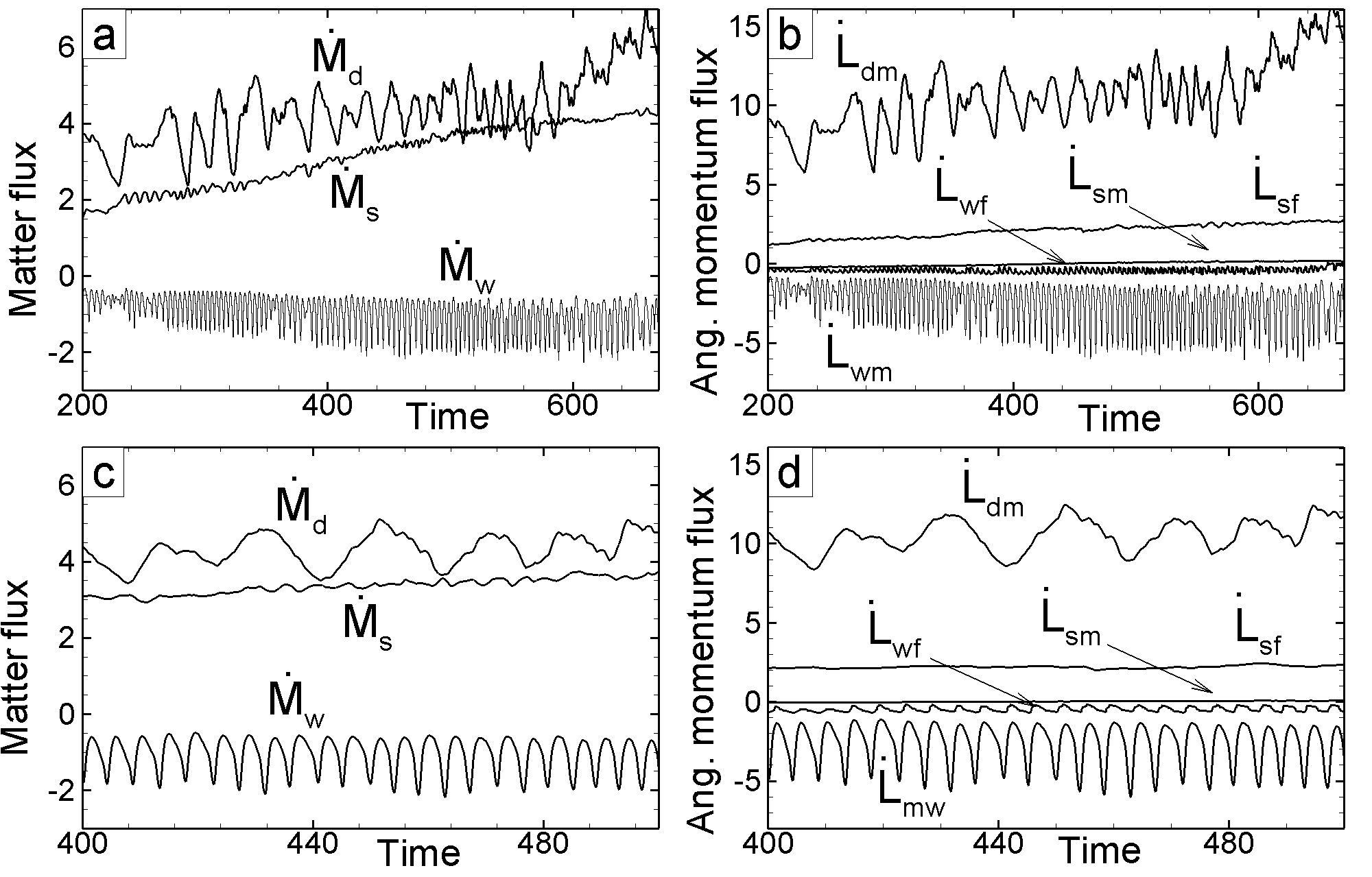
Figure 14: Panel a: matter flux onto the star $\dot{M}_{s}$, into the conical wind $\dot{M}_{w}$, and through the disk $\dot{M}_{d}$. Panel b: angular momentum flux carried by the disk $\dot{L}_{d}$, onto the star carried by matter $\dot{L}_{\rm sm}$ and by the magnetic field $\dot{L}_{\rm sf}$. The angular momentum flux of the conical wind carried by matter is $\dot{L}_{\rm wm}$ and that carried by the field is $\dot{L}_{\rm wf}$. Panels c, d show the time dependence of these fluxes.

4 Analysis of fluxes: matter, energy, angular momentum

4.1 Fluxes in Conical winds

Fig. 12a shows the matter flux distribution $F_{m}$ and a neutral line of the magnetic field where $B_{r}=0$. This line separates the field lines starting on the disk from those starting on the star. One can see that the conical wind flows along both sets of field lines. Panel d shows that the matter flux $F_{m}$ has a sharp peak in its angular distribution (at $r=6$), that is, the wall of the cone is narrow. The position of the $B_{r}=0$ line in this panel shows that matter flows along both the stellar and the disk field lines. For $\theta>75^{\circ}$, the matter flux is dominated by the disk and is negative. We also see that the density $\rho$ is low in the corona. In the disk the density increases to much larger values, $\rho=1-10$. There is also a low-density gap at $\theta\sim 45^{\circ}$ where matter is accelerated to high velocities.

The energy flux ${\bf F}_{\rm E}$ is the sum of the matter component ${\bf F}_{\rm Em}$ and the field component ${\bf F}_{\rm Ef}$ where

$${\bf F}_{\rm Em}=\rho{\bf v}_{p}\left(\frac{1}{2}v^{2}+w+\Phi_{g}\right),~{}~{}{\bf F}_{\rm Ef}=\left(\frac{c}{4\pi}\right)({\bf E}\times{\bf B})_{p},$$ (5)

where $w$ is the enthalpy and $\Phi_{g}$ is the gravitational potential.

Fig. 12b shows that the magnetic field energy flux $F_{\rm Ef}$ is high near the star, at the base of the conical wind and in the region of fast flow. Panel e shows that the energy flux $F_{\rm Ef}$ at $r=6$ has a peak in the region of the conical wind.

Fig. 12c shows that the distribution of the matter energy flux, $F_{\rm Em}$, is similar to the matter flux distribution. The panel also shows that in the conical wind, matter crosses all the critical surfaces. It ends up flowing with a super-fast-magnetosonic velocity. In contrast, in the corona, away from the regions of outflow, the flow is sub-slow-magnetosonic. Panel f shows that the entropy $S$ is high in the corona and low in the conical wind and the disk.

Fig. 13a and d shows the ratio of the gas and magnetic pressures, which is the conventional $\beta$ parameter. We also use what we term the kinetic parameter $\beta_{1}$, where

$$\beta=\frac{p}{B^{2}/8\pi}~{},\quad~{}\beta_{1}=\frac{p+\rho v^{2}}{B^{2}/8\pi}~{}.$$ (6)

The flow region is magnetically dominated when the $\beta$ or $\beta_{1}$ is less than unity. The magnetic pressure dominates only in the region near the star in the conical wind case. The situation is different in the propeller regime where the axial region is magnetically dominated (see §4).

We calculate the angular momentum flux distribution which consists of three components, ${\bf F}_{L}={\bf F}_{\rm Lm}+{\bf F}_{\rm Lf}+{\bf F}_{\rm Lv}$, where ${\bf F}_{\rm Lm}$, ${\bf F}_{\rm Lf}$ and ${\bf F}_{\rm Lv}$ are the angular momentum fluxes carried by the matter, the magnetic field, and the viscosity:

$${\bf F}_{\rm Lm} = r\sin\theta\rho v_{\phi}{\bf v}_{p}~{},\quad\quad{\bf F}_{\rm Lf}=-r\sin\theta\frac{B_{\phi}{\bf B}_{p}}{4\pi}~{},~{}$$

$${\bf F}_{\rm Lv} = -\nu_{t}\rho(r\sin\theta)^{2}{\bf\nabla}\Omega~{}.$$ (7)

Fig. 13b shows that the magnetic component $F_{\rm Lf}$ of the flux, dominates near the star and in the part of the conical wind close to the disk. The streamlines show that angular momentum flows from the disk onto the star, from the disk into the conical wind, and from the star into the corona. Panel c shows that the conical winds carry away angular momentum associated with matter, $F_{\rm Lm}$. The magnetic component is also high at the base of conical wind. However, at larger distances this angular momentum is converted into angular momentum carried by matter. Comparison of panels e and f shows that at $r=6$, the angular momentum carried by the matter is much larger than that carried by the field. Panel e also shows that some angular momentum flows into the disk wind (at $\theta>60^{\circ}$). Panel f shows that the angular momentum carried by viscosity is significant. The disk viscous component is much larger than the matter component flowing into the conical wind, so most of the angular momentum flows outward along the disk.

We also calculated the matter and angular momentum fluxes flowing through the surface of the star, and through a spherical surface of radius $r=6$.

$$\dot{M}=\int d{\bf S}\cdot{\bf F}_{m}~{},\quad\quad{\bf F}_{m}=\rho{\bf v}_{p}~{},$$ (8)

$$\dot{L}=\int d{\bf S}\cdot({\bf F}_{\rm Lm}+{\bf F}_{\rm Lf}+{\bf F}_{\rm Lv})~{},$$ (9)

where $d{\bf S}$ is the surface area element directed outward. Fig. 14 (left panels) shows that about $2/3$ of the incoming disk matter flows to the star, and the rest going into the conical wind. Fluxes into the wind oscillate due to magnetic field inflation and reconnection events. The right-hand panels show that angular momentum flows inward with the disk matter, $\dot{L}_{\rm dm}$. Part of this angular momentum is carried away by the conical wind. Angular momentum is carried mainly by matter, $\dot{L}_{\rm wm}>>\dot{L}_{\rm wf}$. Part of the disk angular momentum flows to the star and spins it up (the star rotates slowly in that $r_{cor}=3$). The angular momentum carried to the star by the matter, $\dot{L}_{\rm sm}$, is converted into angular momentum carried by the field, $\dot{L}_{\rm sf}$, and hence on the surface of the star $\dot{L}_{\rm sf}>>\dot{L}_{\rm sm}$ (see also R02). One can see from Fig. 14 that all these fluxes are smaller than the flux carried by the disk matter. This means that the main part of the angular momentum of the disk flows outward to larger distances due to viscosity.

4.2 Fluxes in the propeller regime

We analyze fluxes in the propeller regime in a similar manner to that for the conical winds. Fig. 15a shows the distribution of the poloidal matter flux $F_{m}$ in the background with the vectors ${\bf F}_{m}$ on top. The neutral line (dashed white line) separates the field lines which start in the disk from those which start on the star.

Panel d shows that most of the matter flows along field lines threading the disk, although some matter flows along the stellar field lines. For $\theta>80^{\circ}$ (in the disk region) the matter flux becomes much larger and negative (we exclude this part of the plot to show the conical wind part more clearly). The plot of the density shows that the density is very low on the axis but gradually increases toward the region of the conical wind and continues to grow towards the disk.

Panel b shows the distribution of the magnetic energy flux $F_{\rm Ef}$. One can see that a strong flux of magnetic energy (Poynting flux) flows into the corona. This is the region where matter is accelerated to high velocities (see velocity vectors). Panel e shows that at $r=10$ the magnetic energy flux is very large, and is distributed over a range of angles with a maximum at $\theta\sim 25^{\circ}$ (not on the axis). The plot also shows that the poloidal velocity is slightly larger than the azimuthal velocity and both velocities are high, up to $v_{p}=2$ (which is $400$ km/s for protostars). The jet component is smaller in the case of slowly rotating stars.

Panel c shows the energy flux associated with the matter flow. One can see that matter in the conical wind crosses the slow magnetosonic surface $v=v_{\rm sm}$ just above the disk, and soon crosses the Alfvén surface $v=v_{A}$, and the fast magnetosonic surface $v=v_{\rm fm}$. Panel f shows that the matter energy flux distribution has a sharp peak in the region of the conical wind and that the entropy $S$ is high in the corona but drops towards the disk.

Comparison of panels e and f shows that the maximum of the energy flux carried by the magnetic field into the jet, $F_{\rm Ef}$, is about 3 times larger than that carried by the matter into conical winds, $F_{\rm Em}$. In addition, the integrated flux carried by the magnetic field is a few times larger. Therefore, the cumulative energy flux carried by the magnetic field into the jet (the Poynting flux) is about 10 times larger than that carried by matter. This means that the jet component is 10 times more powerful. Part of this energy is converted into kinetic energy of the fast component inside the simulation region. However, most of the magnetic energy may be transferred to particles or converted into radiation at larger distances from the star.

Next, we analyze the angular momentum flow. Fig. 16a shows the $\beta$-parameter in the background and the $\beta=1$ and $\beta_{1}=1$ surfaces in the foreground (see equation 6). One can see that the magnetic energy dominates in the whole axial coronal region interior to the conical wind ($\beta_{1}<1$ and $\beta<1$). If one uses only the standard criterion $\beta=1$, then one can see that the region above the disk is also magnetically dominated ($\beta<1$). Panel d shows the angular distribution of $\beta$ and $\beta_{1}$ at $r=10$.

Panel b shows the distribution of the angular momentum flux carried by the magnetic field, $F_{\rm Lf}$, and the streamlines associated with this flux. One can see that a significant amount of angular momentum flux flows from the star into the corona along the stellar field lines. Panel e shows that the angular momentum flows out along the set of field lines between the axis and the neutral field line with a maximum right above the conical wind component. Some of them thread the low-density corona, while others thread the upper part of the conical wind above the neutral line. These panels also show that a significant amount of angular momentum flows from the inner part of the disk. See U06 for detailed analysis of the different components of the angular momentum flow.

Panel c shows that the angular momentum flux carried by the matter is also large and is carried by the conical wind. Panel f shows that most of this angular momentum flows along the disk field lines while some angular momentum flows along the stellar field lines.

Fig. 17a shows the matter fluxes onto the star $\dot{M}_{s}$, and into the outflows, $\dot{M}_{w}$, integrated over a surface with radius $r=10$ (any flow with $v_{r}>0$ is taken into account). One can see that the matter flux into the wind is much larger than that onto the star, $\dot{M}_{w}>>\dot{M}_{s}$, that is, almost all disk matter is ejected from the system into the outflows. Here we should note that we consider the “strong propeller” case, $r_{cor}<<r_{m}$. If the star rotates slower, then the fraction of the matter flux going into the wind decreases, and a larger portion of the matter may accrete onto the star (see U06 for dependences of matter fluxes on $\Omega_{*}$, $B_{*}$, $\alpha_{v}$ and $\alpha_{d}$.) Both fluxes are strongly variable and show episodic enhancement of accretion and outflows. Simulations show that an interval between the strongest outbursts increases when diffusivity coefficient $\alpha_{d}$ decreases (R05, U06).

Panel b shows the integrated angular momentum fluxes through the same $r=10$ surface. Here we calculate separately the angular momentum fluxes carried by the field and by the matter. One can see that the star spins down due to the angular momentum carried by the magnetic field, $\dot{L}_{\rm sf}$, while the angular momentum carried by the matter flow, $\dot{L}_{\rm sm}$, is negligibly small. The angular momentum outflow from the star, $\dot{L}_{\rm sf}$, almost coincides with the angular momentum carried by magnetic field lines into the magnetically-dominated jet, $\dot{L}_{\rm wf}$. This indicates that angular momentum flows from the star into the magnetically dominated axial jet. Thus a star in the propeller regime is expected to spin down rapidly due to angular momentum flow into the magnetically-dominated axial jet. Analysis of U06 shows that this jet angular momentum is approximately equally split between the flux carried into the corona along open field lines, and the flux which flows along partially inflated field lines which close inside the simulation region and are connected with both the star and the disk. Panel c shows that the angular momentum carried by matter into the conical winds, $\dot{L}_{\rm wm}$ is approximately equal to that carried by the field to the corona. The bottom panels show the same plots at higher time resolution. Therefore, the star-disk system loses its angular momentum through both the wind and jet components, via the inner disk and star respectively. So, there is no problem with excess angular momentum in the star-disk-system; it flows into the jet/wind.

5 Other properties of outflows

5.1 Inflation of Field Lines and Disk Oscillations

The field lines connecting the disk and the star have the tendency to inflate (e.g., Lovelace, Romanova & Bisnovatyi-Kogan 1995). Quasi-periodic reconstruction of the magnetosphere due to inflation and reconnection has been discussed theoretically (Aly & Kuijpers 1990; Uzdensky, Litwin & Königl 2003) and has been observed in a number of axisymmetrtic simulations (Hirose et al. 1997; Goodson et al. 1997, 1999; Matt et al. 2002; Romanova et al. 2002 - hereafter R02; von Rekowski & Brandenburg 2004). Goodson & Winglee (1999) discuss the physics of inflation cycles. They have shown that each cycle of inflation consists of a period of matter accumulation near the magnetosphere, diffusion of this matter through the magnetospheric field, inflation of the corresponding field lines, accretion of some matter onto the star, and outflow of some matter as winds, with subsequent expansion of the magnetosphere. There simulations show $5-6$ cycles of inflation and reconnection.

Our simulations show $30-50$ cycles of inflation and reconnection in the propeller regime. We chose one outburst from our simulations and plotted the density and a fixed set of magnetic field lines at different times. Fig. 18 shows that at $T=890$, the magnetosphere is relatively expanded, although some matter accretes around the expanded field lines (see also Romanova et al. 2004a). At $T=900$, the disk matter comes closer to the star and some field lines inflate or partially inflate, thus blocking accretion. At $T=910$ even more field lines inflate and accretion is blocked. However, outflow is permitted at both of these moments of time. At $T=916$, the internal field lines reconnect, permitting accretion onto the star. At $T=921$, the magnetosphere expands and accretion onto the star is again prevented. Later, at $T=927$, the field lines reconnect and some matter accretes along a longer path – around the expanded magnetosphere. This picture is similar to that described by Goodson & Winglee (1999).

Fig. 17d shows that the time interval between the strongest outbursts in the propeller regime is $\Delta T\approx 50-70$. In application to protostars and CTTSs ($P_{0}=1.04$ days) this time corresponds to $(\Delta t)_{\rm outb}=52-73$ days. In some young stars, like CTTS HH30 (XZ Tau), for example, the outbursts into the jet occur at intervals of a few months, which hints that episodic inflation of field lines may be responsible for some outbursts. During the outbursts, the matter flux into outflows increases several times and the velocities also increase. This may lead to the formation of new blobs or to the generation of shock waves in the outflow. This mechanism may be relevant for formation of blobs or shocks in protostars and rapidly rotating CTTSs. In slowly rotating stars, the time-interval between outbursts is smaller, $(\Delta t)_{\rm outb}\approx 5$ days (see Fig. 14), so the outbursts have a smaller amplitude but are more frequent. The interval depends on the diffusivity in the disk, $\alpha_{d}$. At very small diffusivity the time-interval between outbursts may be much larger.

Diffusivity is important for reconnection processes in the corona. We have diffusivity only in the disk. We choose a certain density level $\rho_{d}=0.3$ below which the diffusivity is absent, so that high-density regions, $\rho>0.3$, which correspond to the disk and the funnel streams, have diffusivity, and low-density regions do not. In the corona and the conical outflows, the diffusivity has only a numerical origin and is small. Namely, we observe in simulations that in conical winds, the two layers of plasma with an oppositely directed magnetic field reconnect only slowly. Similar behavior has been observed in ideal MHD simulations by Fendt & Elstner (2000). An anomalous (high) diffusivity was added by Hayashi et al. (1996) to a part of the simulation region to enhance the reconnection process in the inflating plasmoids. Diffusivity had been added into the whole simulation region by Fendt & Cemeljić (2002). They observed that at higher diffusivity the level of collimation by the magnetic field and the Lorentz force decrease, while the centrifugal force increases. We performed exploratory simulations with non-zero diffusivity in the corona. We added to the corona the same diffusivity as in the disk with $\alpha_{d}=0.1-0.2$, which operates at different density levels, $\rho>\rho_{d}$, where $\rho_{d}=0.1,0.03,0.01$ and in the whole simulation region (formally, $\rho_{d}=0$). We observed that in case of conical winds (slowly rotating stars) the diffusivity in the corona does not change the result. However, in case of propeller-driven winds, we observed that propeller becomes weaker. We believe that the difference is in the fact that in the case of conical winds, the wind and the neutral line of the inflated magnetic field have approximately the same position in space, leading to slower reconnection. In the other case, in the propeller regime the inner disk and the region of outflows strongly oscillates, and so the position of the neutral line varies, and hence the reconnection is forced (that is, the plasma layers with oppositely directed fields are pushed towards each other by an external force).

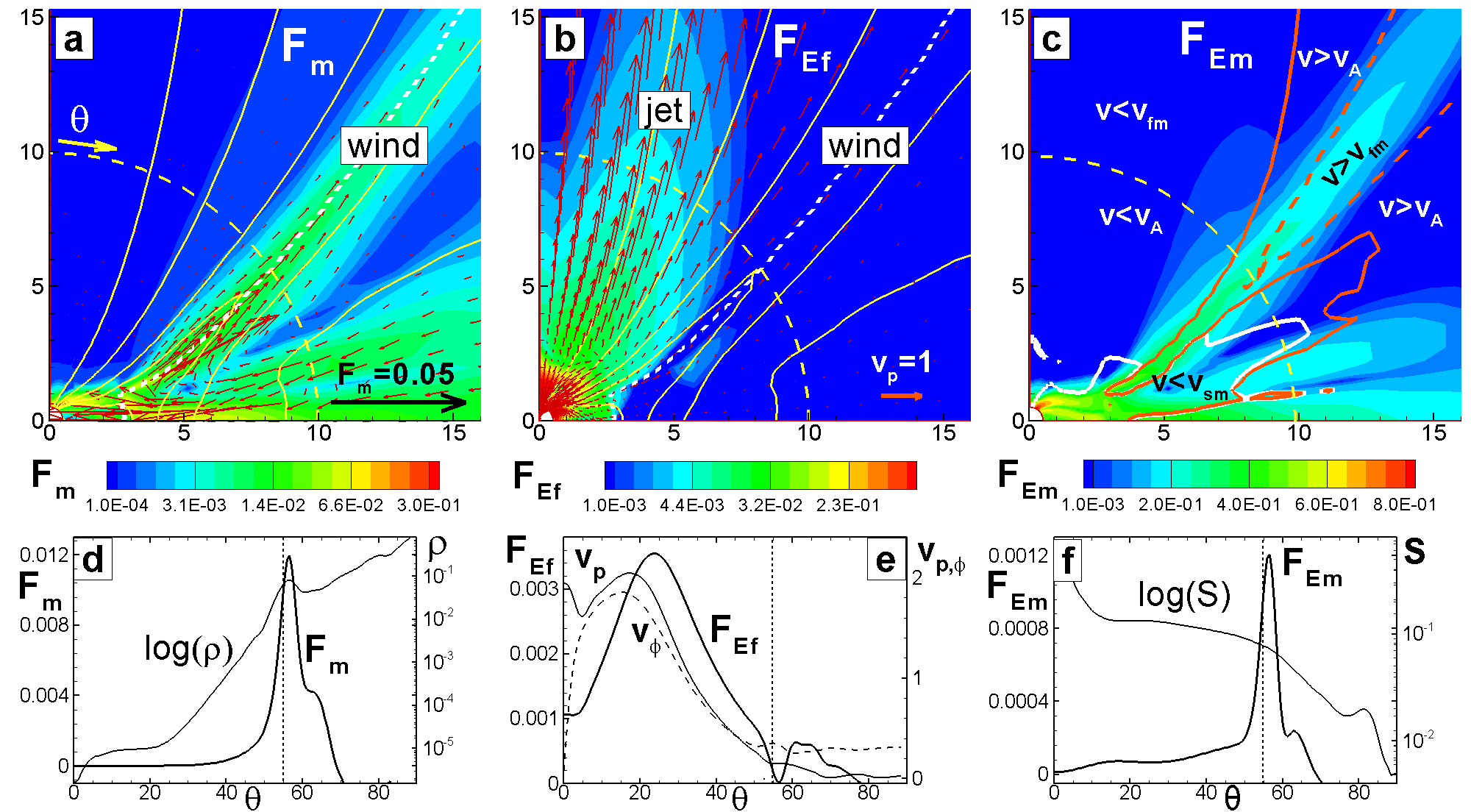
Figure 15: Same as in Fig. 12 but for the propeller regime at time $T=1400$.

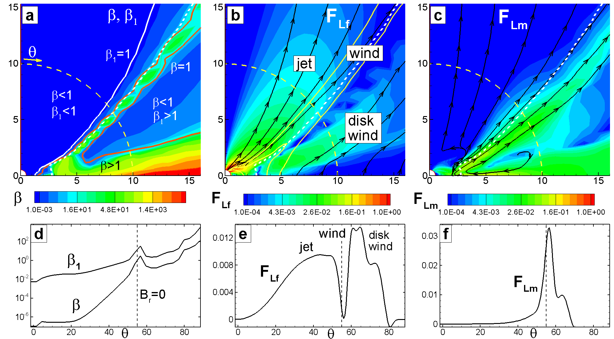
Figure 16: Same as in Fig. 13 but for the propeller regime at time $T=1400$.

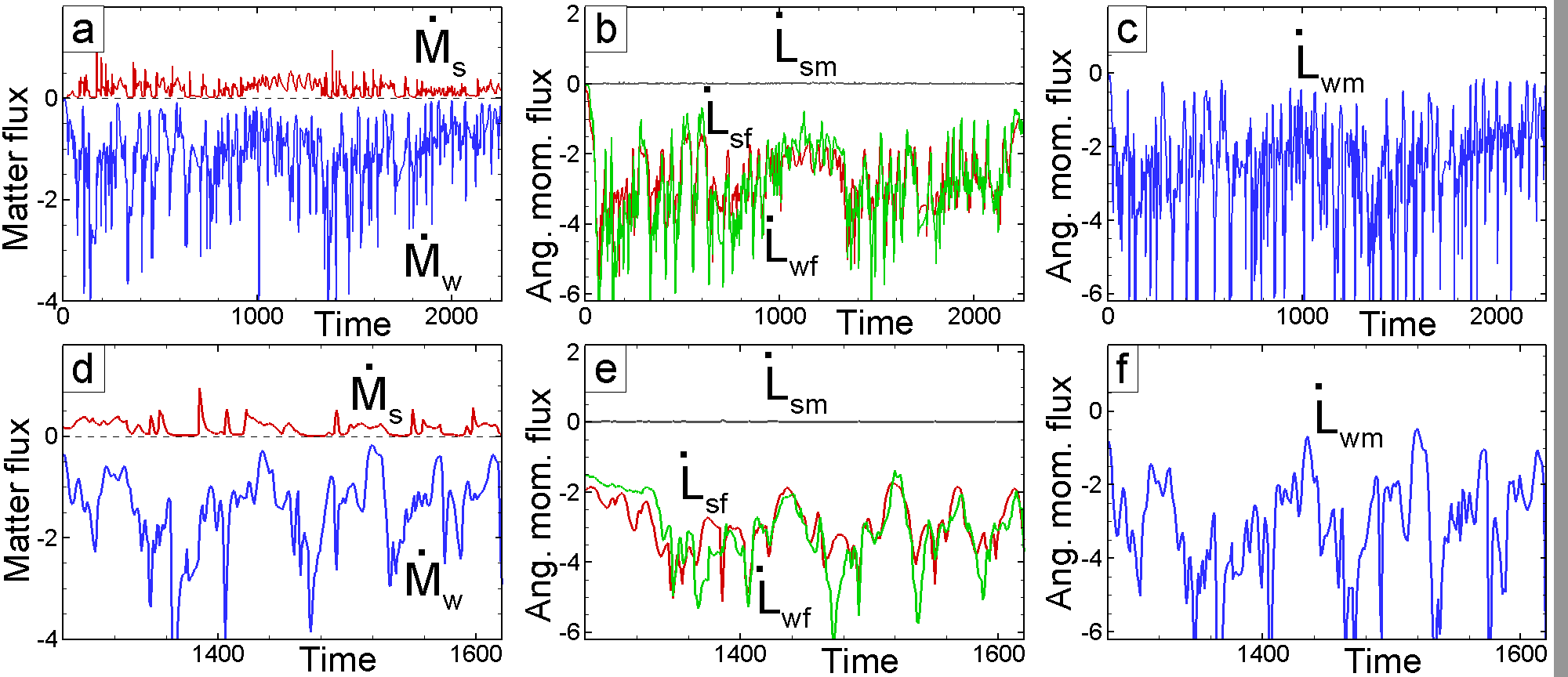
Figure 17: Panel a: matter fluxes onto the surface of the star $\dot{M}_{s}$, and into the outflows (both wind and jet) through the surface $r=10$ versus time $T$. Panel b: angular momentum fluxes carried to (or out from) the star by the matter, $\dot{L}_{\rm sm}$ (gray line), and by the magnetic field, $\dot{L}_{\rm sf}$ (red line). The green line shows the angular momentum flux carried by the magnetic field through the surface $r=10$. Panel c: angular momentum flux carried by the matter component $\dot{L}_{\rm wm}$ through the surface $r=10$. The bottom panels show the same fluxes but during a part of the simulation time.

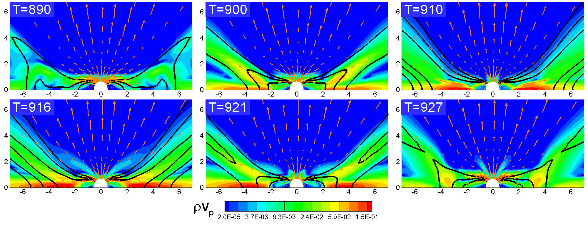
Figure 18: Several snapshots from simulations show the mechanism of enhanced accretion and outflows observed in the light-curves of propeller-driven accretion and outflows. The background shows the matter flux, lines are the sample magnetic field lines, the same set of which is shown in all plots.

5.2 Matter loading onto stellar field lines, and possible role of stellar wind

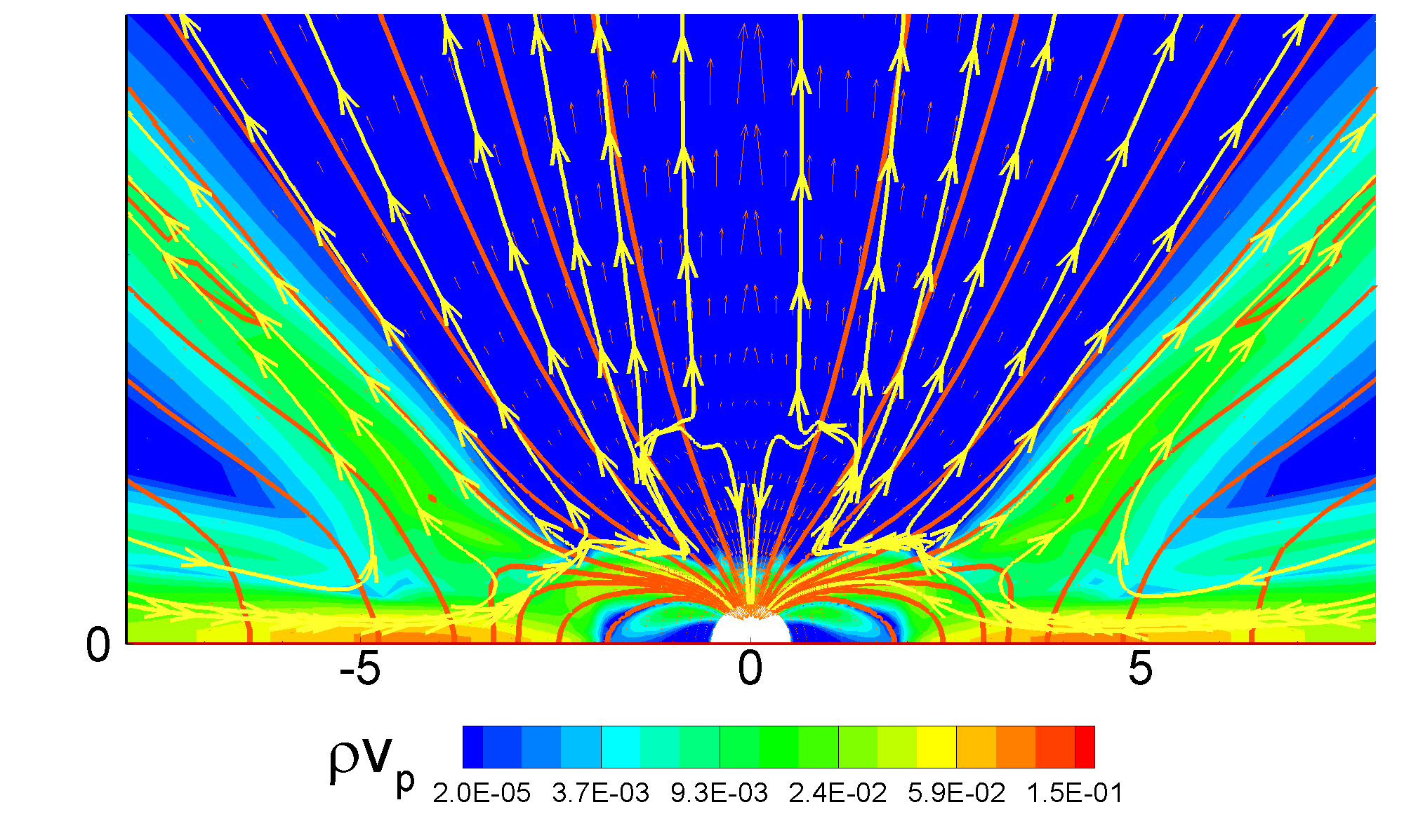
Figure 19: White lines with arrows show streamlines of matter flow in the propeller regime at $T=1500$. Red lines show sample magnetic field lines. Only the inner part of the simulation region is shown.

Here we discuss how the disk matter gets loaded onto the stellar field lines and then flows into the jet in the propeller regime (where the jet is strong). It is important to have diffusivity in the disk, so that the matter of the disk threads the field lines of the star and flows onto the star in funnel streams. When a sufficient amount of matter is accumulated in the inner disk, the field lines connecting the star and the disk inflate. During and after inflation, part of the disk matter ends up on the field lines connecting the disk with corona (usually most of the matter flows along these field lines). Another, smaller part of the matter ends on the field lines connecting the star with the corona. For example, Fig. 15a demonstrates the result of such inflation, where the neutral line dividing the stellar and disk lines is in the middle of the conical wind component. On the other hand, when matter flows in a funnel stream, most of it accretes onto the star. However, part of it is stripped away by the magnetic and centrifugal forces and flows into the jet along the stellar field lines. Fig. 19 shows that there is a dividing line running through the upper part of the funnel stream, separating the regions from which matter flows onto the star (most of it) from those from which it flows into the jet along the stellar field lines (a small fraction). In the funnel region the density is usually high enough so that the diffusivity which works in our disk also works in the funnel stream. This diffusivity helps launch matter from the funnel stream field lines onto the coronal, jet field lines. Both processes are consistent with the strong decrease in coronal matter density along the axis. This region is “matter-starved”.

Our simulations do not take into account possible stellar winds. Even a weak wind from the star may have a significant influence on the axial region of the jet in the propeller regime and the “matter-starved” jet region in slowly rotating stars. The existence of powerful stellar winds was suggested by Matt & Pudritz (2005, 2008) in order to explain the loss of angular momentum by young stars. The spectra of many CTTSs (e.g. Edwards et al. 2003; Dupree et al. 2005) require up to 10% of the disk mass flowing out as winds, in order to explain different spectral lines (Edwards 2009). No such winds are observed in diskless, weak-line T Tauri stars. Hence, the winds must be accretion-driven (e.g., Edwards et al. 2006; Kwan et al. 2007). The physics of these accretion-driven stellar winds is not understood yet. In the standard approach it is suggested that matter falling onto the surface of the star through the funnel stream forms a shock near the surface and is heated by this shock. However, it cools rapidly in the radiative zone behind the shock wave, and no reverse flow into the wind is expected (e.g., Lamzin 1998; Koldoba et al. 2008). In another investigation, however, Alfvén waves and other processes at the stellar surface help accelerate up to $1\%$ of the accreting disk matter into the wind (e.g. Cranmer 2008). We did not incorporate stellar winds into the present simulations. Weak winds may help supply matter to the magnetically-accelerated axial jets and the “matter-starved” region of fast flow in slowly rotating stars. On the other hand, if the wind is very strong, say $\dot{M}_{sw}\sim 0.1\dot{M}_{d}$, it will probably be matter-dominated at moderate distances from the star (say $\gtrsim 10$ stellar radii) and will have a decollimating effect on the outflows (Fendt 2009). In summary, a weak stellar wind will contribute matter to the jet component.

5.3 Collimation of outflows

Collimation of conical winds.

We observe conical winds in both slowly and rapidly rotating stars. In both cases, matter in the conical winds passes through the Alfvén surface, beyond which the flow becomes matter-dominated. We note that in slowly rotating stars, the distribution of the poloidal current $J_{p}$ (see Fig. 5c) is such that the corresponding magnetic force has a component towards the axis. This may explain why conical winds show some collimation (see Fig. 2). The conical wind component of the propeller-driven outflows shows stronger collimation during periods of inflation and outbursts (see Fig. 8). However, this collimation may not be sufficient to explain well-collimated jets.

Conical winds may be further collimated at larger distances from the star either by the pressure of the external medium (Lovelace et al. 1991; Frank & Mellema 1996), or by disk winds (Königl & Pudritz 2000; Ferreira et al. 2006; Matsakos et al. 2008; Fendt 2009). In addition, Matt, Winglee, & Böhm (2003) have shown that a weak axial magnetic field ($B<<0.1$ G) associated with the disk, may collimate the winds at a distance of a few AU.

Collimation of the jet.

In the propeller regime, the jet component is self-collimated by the magnetic hoop-stress. The level of collimation increases towards the axis. The poloidal velocity in the jet also increases towards the axis, and varies between $v_{p}\approx 2$ near the axis and $v_{p}\approx 0.2$ near the conical wind. That is why we choose a few typical velocity levels $v_{p}=v_{c}$, with $v_{c}=0.5,1$ and $1.5$, and plot lines of equal velocity (Fig. 20). In application to protostars, the fast component of the jet, $v_{p}\gtrsim 200$ km/s, carries $\sim 2\%$ of the mass and $\sim 22\%/0.6\approx 37\%$ of the angular momentum flux out of the star. At the lower velocity limit, $v_{p}\gtrsim 100$ km/s, these numbers are $10\%$ and $35\%/0.6\approx 60\%$.

It is of interest to know the dependence of the mass outflow rate on the poloidal velocity $v_{p}$. We calculate the matter flux $\dot{M}(v_{p}>v_{c})$ through the external boundary $r=R_{out}$ at poloidal velocities above a certain value $v_{c}$ for different values of $v_{c}$. Panel a shows that the jet component with $v_{p}>0.5$ carries about $10\%$ of the total outflowing mass $\dot{M}_{w}$, while the very fast components, $v_{p}>1.5$ and $v_{p}>1$ carry only about $1\%$ and $2\%$ correspondingly. So, about $10\%$ of the total mass flows into the collimated jet. The fractions of matter flowing into different parts of the jet and into the conical wind are shown in the left panel.

The jet carries angular momentum out of the star along different field lines corresponding to different $v_{p}$. It is of interest to know which part of the jet carries most of the angular momentum. We calculate the angular momentum flux carried by the magnetic field $\dot{L}_{f}(v_{p}>v_{c})$ (this component dominates in the jet) through the external boundary and normalize it to the total magnetic flux through this boundary, $\dot{L}_{\rm wf}$. Panel b shows that the high-velocity part of the jet, $v_{p}>1.5$, carries about $13\%$ of the total angular momentum flux, while the entire inner part of the jet in the velocity intervals $v_{p}>1$ and $v_{p}>0.5$ carry $22\%$ and $35\%$ of the flux correspondingly. Another fraction ($12\%$) flows out along stellar field lines threading the conical wind component and the low-velocity area above it. All this flux is responsible for spinning down the star (which is about $60\%$ of the total flux). The rest of the flux ($40\%$) flows along the disk field lines threading the conical winds and the disk. We conclude that the jet component above the conical wind carries a relatively small mass but has a significant contribution to the angular momentum outflow from the star. Note that only about half the star’s angular momentum flows into the jet. The other half is associated with star-disk interaction through the field lines which are closed inside the simulation region and were not taken into account in this analysis (see U06 for details). In application to protostars, the fast component of the jet, $v_{p}\gtrsim 200$ km/s, carries $\sim 2\%$ of the mass and $\sim 22\%/0.6\approx 37\%$ of the angular momentum flux out of the star. At the lower velocity limit, $v_{p}\gtrsim 100$ km/s, these numbers are $10\%$ and $35\%/0.6\approx 60\%$.

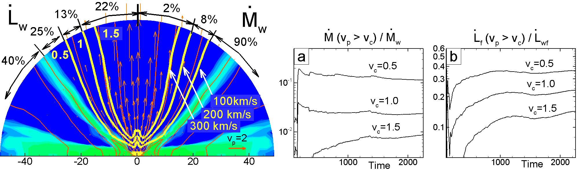
Figure 20: Analysis of matter and angular momentum distribution between the jet and wind components in the propeller regime at $T=1400$. Left panel: The yellow lines show surfaces of constant poloidal velocity, $v_{c}=0.5,1,1.5$ ( in application to protostars they are approximately $100$, $200$ and $300$ km/s). Numbers on top of the plot show fractions of total matter flux $\dot{M}_{w}$ into different sectors of the region, and the same for angular momentum carried by the field, $\dot{L}_{\rm wf}$. Panel b: Matter flux into the jet through an external boundary, $r=R_{out}$, with velocities $v_{p}>v_{c}$, $\dot{M}(v_{p}>v_{c})$ versus total matter flux $\dot{M}_{w}$. Panel c: Same as in panel b, but for the angular momentum flux carried by the magnetic field.

6 3D Simulations of Conical Winds

We did exploratory simulations of conical winds in global 3D simulations. We chose a case where the dipole magnetic field of the star is misaligned with the rotation axis (of the star and disk) by an angle $\Theta=30^{\circ}$. One question is what the direction of the conical wind is in the case of an inclined dipole. We used the Godunov-type 3D MHD “cubed sphere” code developed by Koldoba et al. (2002). In the past we have used this code to study magnetospheric accretion close to the star (Romanova et al. 2003, 2004b). Compared with that work we decreased the density in the corona by a factor of $10$ to $\rho_{c}=0.001$ and created conditions suitable for bunching of the field lines. We used a grid resolution of $N_{r}\times N^{2}=120\times 51^{2}$ in each of 6 blocks of the sphere. We took the density in the disk to be $\rho_{d}=2$ which is $5$ times lower than in the axisymmetric case shown above. At the same time, we chose a smaller magnetic moment for the star, $\mu=2$ compared to $\mu=10$ in the axisymmetric case (to reduce the computing time). We start the disk flow not from large distances but from $r=5$, to limit the computing time. The bunching of field lines is achieved by having a sufficiently high viscosity, $\alpha_{v}=0.3$. We do not have diffusivity in the 3D code, but at the grid resolution we use, the estimated numerical diffusivity at the disk-magnetosphere boundary is at the level of $\alpha_{d}\sim 0.01-0.02$, and hence the main condition for conical wind formation, Pr${}_{m}\gtrsim 1$, is satisfied (see also Appendix C).

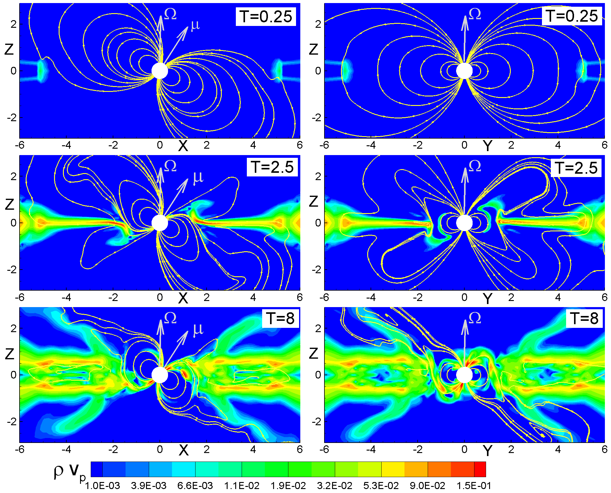
Figure 21: Projections show formation of conical winds obtained in 3D MHD simulations. Left panels show the distribution of matter flux (background) and sample magnetic field lines in the XZ plane at different moments of time. Right panels show corresponding YZ slices. Arrows show the direction of the magnetic moment of the star $\mu$ and angular velocity of rotation $\Omega_{*}$.

Simulations show that the accreting matter bunches up field lines and some matter flows out as a conical wind. Fig. 21 shows that the wind is geometrically symmetric about the rotation axis. However, the density distribution in the wind shows a spiral structure which rotates with the angular velocity of the star, $\Omega_{*}$, and represents a one-armed spiral wave from each side of the outflow.

Note that for high $\alpha_{v}$ ($0.3$ in this case), the disk-magnetosphere boundary may exhibit the magnetic interchange instability (Romanova, Kulkarni & Lovelace 2008; Kulkarni & Romanova 2008). In these simulations we do observe some accretion due to this instability in addition to the main funnel stream accretion that dominates at high misalignment angles, $\Theta\gtrsim 30^{\circ}$ (Kulkarni & Romanova 2009). However, the conical wind originates at larger radii compared with the inner disk radius where accretion through instability dominates. We believe that both processes can “peacefully” co-exist for $\Theta\gtrsim 30^{\circ}$. However, in other situations the conical wind may be influenced by the interchange instability. For example, we did not try to investigate outflows at small $\Theta$ where accretion through instability often dominates. Accretion through instability opens up a new path for penetration of matter through the magnetosphere, and thus may possibly decrease the bunching of field lines and consequently the strength of conical winds. This interrelation between instabilities and conical winds needs to be investigated in future 3D simulations. Longer simulations should be performed, and accretion to rapidly rotating stars should also be examined.

7 Comparison with the X-wind model

Winds from the disk-magnetosphere boundary have been proposed earlier by Shu and collaborators and referred to as X-winds (e.g., Shu et al. 1994). In this model, X-winds originate from a small region near the corotation radius $r_{cor}$, while the disk truncation radius $r_{t}$ (or, the magnetospheric radius $r_{m}$) is only slightly smaller than $r_{cor}$ ($r_{m}\approx 0.7r_{cor}$, Shu et al. 1994). It is suggested that excess angular momentum flows from the star to the disk and from there into the X-winds. The model aims to explain the slow rotation of the star and the formation of jets. In the simulations discussed here we have obtained outflows from both slowly and rapidly rotating stars. Both have conical wind components which are reminiscent of X-winds. What, then, is the difference between X-winds, conical winds and propeller-driven winds?

In some respects conical/propeller winds are similar to X-winds: (1) They both require bunching of the poloidal field lines and show outflows from the inner disk; (2) They both have high rotation and show gradual poloidal acceleration (e.g., Najita & Shu 1994).

The differences are the following: (1) The conical/propeller outflows have two components: a slow high-density conical wind (which can be considered as an analogue of the X-wind), and a fast low-density jet. No jet component is discussed in the X-wind model. (2) Conical winds form around stars with any rotation rate including very slowly rotating stars. They do not require fine tuning of the corotation and truncation radii. For example, bunching of field lines is often expected during periods of enhanced or unstable accretion when the disk comes closer to the surface of the star and $r_{m}<<r_{cor}$. Under this condition conical winds will form. In contrast, X-winds require $r_{m}\approx r_{cor}$.  (3) The base of the conical wind component in both slowly and rapidly rotating stars is associated with the region where the field lines are bunched up, and not with the corotation radius. (4) X-winds are driven by the centrifugal force (Blandford & Payne 1982), and as a result matter flows over a wide range of directions below the “dead zone” (Shu et al. 1994; Ostriker & Shu 1995). In conical winds the matter is driven by the magnetic force (Lovelace et al. 1991) which acts such that the matter flows into a thin shell with a cone angle $\theta\sim 30^{\circ}$. The same force acts to partially collimate the flow. (5) In the X-wind model it is suggested that angular momentum flows from the star to the disk in spite of the fact that the truncation radius of the disk is located at $r_{m}\approx 0.7r_{cor}$ and the disk rotates faster than the star (Shu et al. 1994). Simulations show that if the funnel stream starts at $r_{m}<r_{cor}$, then angular momentum flows from the disk to the star along magnetic field lines of the funnel stream which form a leading spiral, and the star spins up (R02, Romanova et al. 2003; Bessolaz et al. 2008). The star may transfer its angular momentum to the disk if $r_{m}>r_{cor}$, like in the propeller case considered above.  (6) The X-wind regime is somewhat similar to the propeller regime, where the star transfers part of its angular momentum to the disk, and this excess angular momentum may flow into the conical component of the wind. However, in the propeller regime, angular momentum also flows from the star into the jet. (7) Conical and propeller-driven winds are non-stationary: the magnetic field constantly inflates and reconnects. X-winds, on the other hand, are steady. This difference, however, is not significant, and models can be compared using time-averaged characteristics.

8 Application to different stars

8.1 Application to Young Stars

Our simulation results can be applied to different types of young stars, including low-mass protostars (class I YSOs) which often show powerful outflows, CTTSs (class II YSOs) which show less powerful outflows, EXors which show periods of strongly enhanced accretion and outflows, and young brown dwarfs.

8.1.1 Low-mass protostars (class I YSOs)

Class I protostars are young stars which are usually embedded inside a cloud of gas and dust. IR observations show that protostars are surrounded by cold massive disks and that the accretion rate is usually an order of magnitude larger than in CTTSs, that is, $\dot{M}\sim(10^{-6}-10^{-7})M_{\odot}/$yr (e.g., Nisini et al. 2005). The outflows are also more powerful than in CTTSs. The stars are fully convective, and so rapid generation of a magnetic field that may even be larger than in CTTSs is expected.

We consider a protostar of mass $M_{0}=M=0.8M_{\odot}$, radius $R_{*}=2R_{\odot}$, and surface magnetic field $B_{*}=3\times 10^{3}~{}{\rm G}$. The dimensionless radius of the star (the inner boundary) is $0.5$, and the unit radius $R_{0}=2R_{*}=2.8\times 10^{11}~{}{\rm cm}$. The velocity scale is $v_{0}=(GM/R_{0})^{1/2}=195$ km/s, the time-scale is $t_{0}=R_{0}/v_{0}=0.16$ days, and the period of rotation at $R_{0}=1$ is $P_{0}=1.04$ days. We take a rapidly rotating star with period $P_{*}=1.04$ days (the corotation radius of $r_{cor}=1$). The other reference variables are shown in Table 1. For dimensionless temperatures in the disk and corona of $\tilde{T}_{d}=5\times 10^{-4}$ and $\tilde{T}_{c}=0.5$, we obtain corresponding initial dimensional temperatures: $T_{d}=2290$ K and $T_{c}=2.3\times 10^{6}$ K. Fig. 22 shows the distribution of density and velocity around the protostar. The age of protostars is $10^{5}-10^{6}$ years, and therefore they may rotate more rapidly than CTTSs and it is likely that some of them are in the propeller regime. If the propeller is strong enough (like in our simulations, where the period $P_{*}\approx 1$ day and $\alpha_{v}=0.3$) then most of the disk matter will be ejected as slow conical winds with velocity $v_{p}\sim 50$ km/s, which may be higher if the disk is closer to the star. Most of the energy, however, flows into the magnetically-dominated axial jet, where a small fraction (about $10\%$) of the disk matter is accelerated up to $v_{p}\sim 100-400$ km/s inside the simulation region. A huge amount of angular momentum flows out of the star through the same jet, and conical winds carry a comparable amount of angular momentum as well. This may solve the angular momentum problem of the system. So, at this stage the outflows are powered by two things: the stellar rotational energy and the inner disk winds (the conical winds). Fig. 17b shows that the outflow is strongly non-stationary with strong matter ejection into jets/winds every $2-3$ months. Ejection is accompanied by larger than average matter flux and velocities, and hence formation of new blobs or shock waves is expected.

A protostar in the propeller regime loses its angular momentum to an axial jet. From the right-hand panels of Fig. 17, we obtain the dimensionless value of the angular momentum loss: $\tilde{\dot{L}}_{sw}\approx 3$, which corresponds to a dimensional value of $\dot{L}_{sw}=\tilde{\dot{L}}_{sw}\dot{L}_{0}\approx 9.3\times 10^{37}~{}{\rm gcm^{2}/s^{2}}$. The star’s angular velocity is $\Omega_{*}=2\pi/P_{*}\approx 7\times 10^{-5}{\rm s}^{-1}$, its angular momentum is $J=kMr^{2}\Omega_{*}=2.2\times 10^{51}k~{}{\rm gcm}^{2}/{\rm s}$, where $k<1$. Taking $k=0.4$, the spin-down time-scale is $\tau=J/{\dot{L}}_{sw}\approx 3\times 10^{5}$ years. Note that this time-scale is calculated for $B_{*}=3\times 10^{3}{\rm G}$. The time-scale decreases with the magnetic field of the star as $\sim B_{*}^{-1.1}$ (see U06) and will be $\tau\approx 3\times 10^{6}$ years for $B_{*}=10^{3}{\rm G}$. If the magnetic field is weaker, then the protostar will continue to spin rapidly even in the CTTSs stage. U06 present the dependence of the spin-down time-scale on the magnetic field, the spin of the star and other parameters.

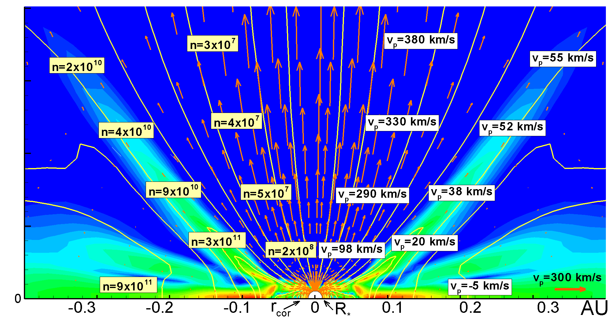
Figure 22: A dimensional example of matter flow in the protostar regime shown in Fig. 9. Time $T=1400$ corresponds to 3.8 years. Labels show the particles density $n$ in units of $1/cm^{3}$ and the poloidal velocity $v_{p}$. Azimuthal velocity is a few times larger that the poloidal velocity in the beginning of the flow, but decreases at larger distances (see Fig. 9).

8.1.2 Classical T Tauri Stars (class II YSOs)

CTTSs and their jets have been extensively studied in recent years. High-resolution observations of CTTSs show that the outflows often have an “onion-skin” structure, with better-collimated, higher-velocity outflows in the axial region, and less-collimated, lower-velocity outflows at a larger distance from the axis (Bacciotti et al. 2000). In other observations, high angular resolution [FeII] $\lambda~{}1.644\mu$m emission line maps taken along the jets of DG Tau, HL Tau and RW Aurigae reveal two components: a high-velocity well-collimated extended component with velocity $v\sim 200-400$ km/s, and a low-velocity, $v\sim 100$ km/s, uncollimated component closer to the star (Pyo et al. 2003, 2006). High-resolution observations of molecular hydrogen in HL Tau have shown that at small distances from the star, the flow shows a conical structure with outflow velocity $\sim 50-80$ km/s (Takami et al. 2007). In XZ Tau, two-component outflows are observed: one component is a powerful but low-velocity conical wind with an opening angle of about $1$ radian, and the other is a fast well-collimated axial jet (e.g., Krist et al. 2008). The origin of these outflows is not known, but we can suggest that at least the lower-velocity component may be explained by the conical winds suggesting that the condition for bunching, Pr${}_{m}>1$, is satisfied. If a CTTS rotates rapidly (in the propeller regime) then the jet component may originate from the propeller effect.

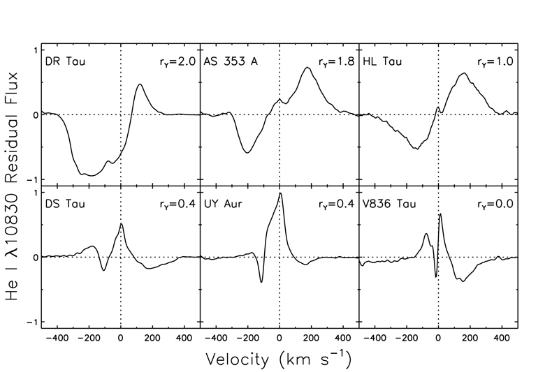
Figure 23: Examples of HE I $\lambda$10830 residual profiles and corresponding 1$\mu$ veiling, $r_{\gamma}$, for 6 accreting CTTSs. The upper row shows high veiling objects with P Cygni profiles characterized by deep and broad blue absorption which is a sign of the high-velocity outflow. The lower row shows low veiling objects with narrow blue absorption which is a sign of a low-velocity outflow. The latter also show red absorption from magnetospheric infall (from Edwards 2009).

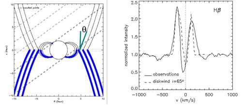
Figure 24: Modeling of the $H_{\beta}$ line in RW Aurigae led to the conclusion that a cone-shaped wind with half-opening angle $30-40^{\circ}$ and a narrow annulus gives the best match to the observations of this line (from Alencar et al. 2005).

Spectral observations of the He I (10830A) line show clear evidence of two-component outflows (Edwards et al. 2003, 2006; Kwan et al. 2007). Observations show (see Fig. 23) that at smaller accretion rates only the relatively low-velocity component, $v\lesssim 100$ km/s, appears. At higher accretion rates there is evidence of a very fast component with $v\sim$ 200-400 km/s which requires an outflow rate of up to $\dot{M}_{w}\sim 0.1\dot{M}_{d}$ (Edwards et al. 2006; Edwards 2009). We suggest that the low-velocity component may be a conical wind. However, it is not clear what can explain the high-velocity component. Even if a star is in the propeller regime, then at the required velocities $v>200$ km/s, only (2-3)% of the disk matter flows into the jet. Possibly, additional matter influx from the wind of the star may enhance the matter flux into the jet component. In another example, observations of the $H_{\beta}$ spectral line in RW Aurigae, and comparison of possible outflow geometries led to the conclusion that a thin cone-shaped wind with a half-opening angle of $30^{\circ}-40^{\circ}$ gives the best fit to the observations (from Alencar et al. 2005; see Fig. 24).

The strongest outbursts supplying CTTS jets are usually episodic or quasi-periodic (e.g., Ray et al. 2007). For example, blobs are ejected every few months in HH30 (XZ Tau), and every 5 years in DG Tau (Pyo et al. 2003). Both of these may be connected with episodes of enhanced accretion and formation of conical winds. The velocity and density in the outflow are larger during periods of enhanced accretion, because the disk comes closer. If the CTTS is in a binary system, then the accretion rate may be episodically enhanced due to interaction with the secondary star, and this may explain the longer intervals of a few years) between outbursts observed in other CTTSs. Events of fast, implosive accretion are also possible due to thermal or global magnetic instabilities (e.g., Lovelace et al. 1994). Alternatively, a period of a few months may be connected with long-term episodes of oscillations of the magnetosphere. In the propeller regime the time-interval between oscillations is 1-2 months even for mild parameters. Bouvier et al. (2007) have shown that magnetospheric expansion in the CTTS AA Tau may occur with a period of a few weeks. Multi-year observations of variability in CTTSs show that they are strongly variable on different time-scales (e.g., Herbst et al. 2004; Grankin et al. 2007) which is probably connected with periods of enhanced accretion.

For CTTSs we suggest the same parameters as for protostars but take a weaker magnetic field, $B=10^{3}$ G, so that for the same dimensionless runs we obtain lower accretion rates (see Table 1). Taking from Fig. 14c the dimensionless values of the matter flux onto the star, $\tilde{\dot{M}_{s}}\approx 3.8$, and into the conical winds, $\tilde{\dot{M}_{w}}\approx 1.3$, and taking the value of $\dot{M}_{0}$ Table 1, we obtain an accretion rate onto the star of $\dot{M}_{s}=\tilde{\dot{M}_{s}}\dot{M}_{0}\approx 7.6\times 10^{-8}~{}{\rm M_{\odot}/yr}$ and into the wind of $\dot{M}_{w}\approx 2.6\times 10^{-8}~{}{\rm M_{\odot}/yr}$. For a corotation radius of $r_{cor}=3$, the period of the CTTS is $P_{*}=$ 5.6 days. In typical simulation run the truncation radius $r_{m}\approx 1.2$ is much smaller than the corotation radius $r_{cor}=3$. This situation corresponds to the case of enhanced accretion when the star spins up, and which corresponds to ejection of conical winds.

Many CTTSs are expected to be in the rotational equilibrium state, when $r_{m}\approx r_{cor}$. Without the bunching condition, and at small viscosity and diffusivity parameters, no significant outflows had been observed in simulations (R02; Long et al. 2005). On the other hand, if the bunching condition is satisfied and/or the accretion rate is enhanced, then conical winds are expected. It is possible that the jet component is also powerful enough in this state so as to produce the fast jet component that is observed. Additional simulations are needed for better understanding of outflows in this important state.

8.1.3 Periods of enhanced accretion and outflows in EXors

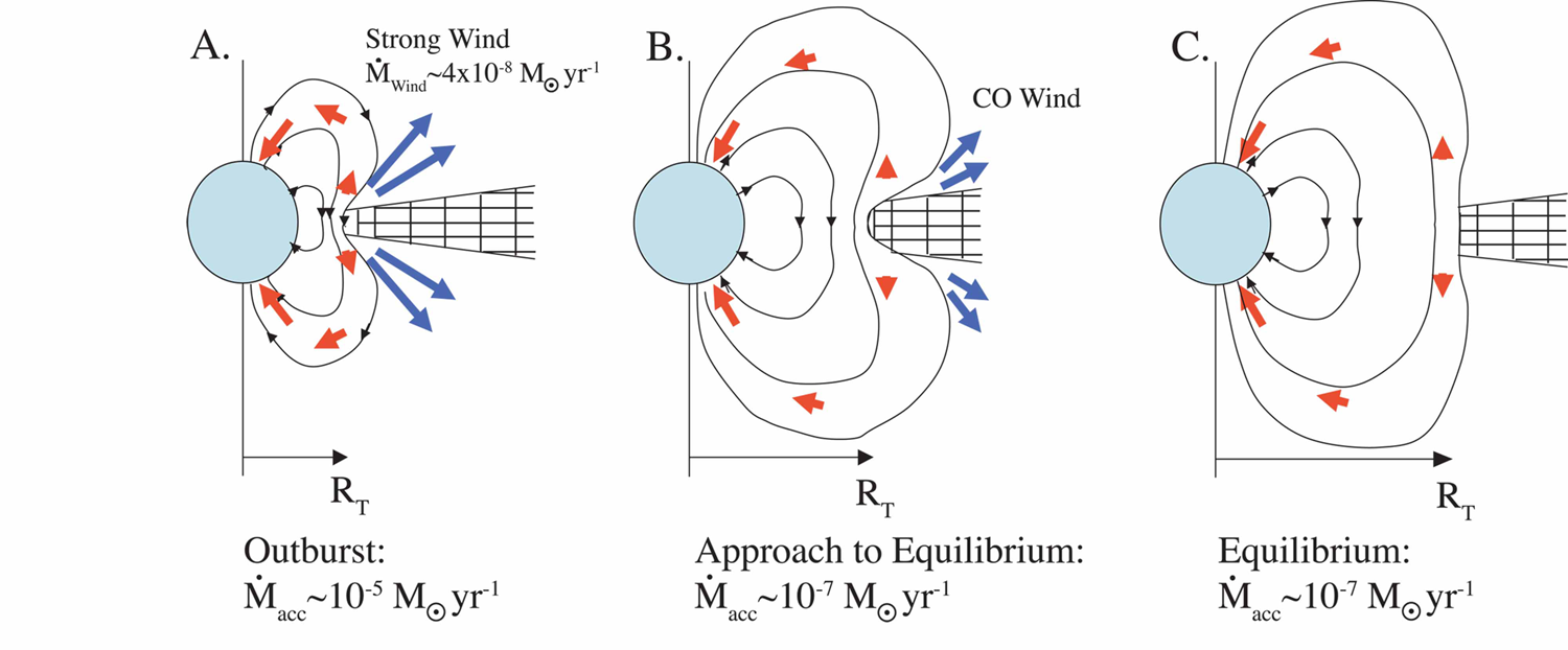
Figure 25: Schematic model of an Exor V1647 Ori. During the outburst the accretion rate is enhanced, and the magnetospheric radius $r_{m}$ decreases and the magnetic field lines are bunched up (A). This results in a fast, hot outflow. As the accretion rate decreases, the disk moves outward and this results in a slower, cooler CO outflow (B). Further decrease in the accretion rate leads to a quiescent state where the production of warm outflows stops (C). From Brittain et al. (2007)

EXors represent an interesting stage of evolution of young stars where the accretion rate is strongly enhanced and powerful outflows are observed (e.g., Coffey, Downes & Ray 2004; Lorenzetti et al. 2006; Brittain et al. 2007). Brittain et al. (2007) reported on the outflow of warm gas from the inner disk around EXor V1647, observed in the blue absorption of the CO line during the decline of the EXor activity. They concluded that this outflow is a continuation of activity associated with early enhanced accretion and bunching of the magnetic field lines (see Fig. 25). The EXor stage may correspond to the initial stage of our simulations, during which a significant amount of matter comes into the region. Or, it is more probable that initially there is weak outflow at the level of that in CTTSs, but later the accretion rate increases by a few orders of magnitude, leading to a powerful outburst which produces conical winds. For conversion into dimensional values, we suggest that the disk comes close to the stellar surface, which is at $r=1$ (as opposed to 0.5 in the previous examples), and the disk stops much closer to the star ($r_{m}=1.2R_{*}$). Then all velocities are higher by a factor of $\sqrt{2}\approx 1.4$, densities by a factor of $32$, and matter fluxes by a factor of $11$ than in the main example relevant to CTTSs.

8.1.4 Outflows from Brown Dwarfs

Recently outflows were discovered from a few brown dwarfs (BDs) (e.g., Mohanty, Jayawardhana & Basri 2005; Whelan, Ray & Bacciotti 2009). Clear signs of CTTS-like magnetospheric accretion (broad spectral lines with full-widths of $v>200$ km/s) were reported earlier for a number of young BDs (e.g., Natta et al. 2004). BDs are fully or partially convective and the generation of a strong magnetic field is expected (Chabrier et al. 2007). Magnetic fields of the order of $0.1-3$ kG may explain the observed properties of magnetospheric accretion (Reiners, Basri & Christensen 2009). Recently, radio pulses were discovered from the L dwarf binary 2MASSW J0746425+200032 with period $P\approx 124$ minutes, which point to a magnetic field of $B\approx 1.7$ kG (Berger et al. 2009). The accretion rates in young BDs are smaller than in CTTS: $\dot{M}=10^{-11}-10^{-9}M_{\odot}/$yr, and are often strongly variable. For example, in 2MASSW J1207334-393254, $\dot{M}$ varied by a factor of $5-10$ during a $6-$ week period (Scholz, Jayawardhana & Brandeker 2005). We suggest that outflows may form in BDs during periods of enhanced accretion or in the propeller regime if the BD is rapidly rotating.

As an example we consider a BD with mass $M_{BD}=60M_{J}=0.056M_{\odot}$, radius $R_{BD}=0.1R_{\odot}$, and surface magnetic field $B_{BD}=2$ kG and obtain the reference parameters shown in the Table 1. The period of the star is another independent parameter. Here we suggest $r_{cor}=2$ which corresponds to $P_{*}=0.13$ days, which is a typical period for a BD. We also suggest that in Fig. 3 the star’s radius is $r=0.5$, that is, the disk is truncated at $r_{m}=1.2/0.5=2.4R_{*}$. For these parameters we obtain an accretion rate of $\dot{M}_{BD}\approx 1.8\times 10^{-10}{\rm M_{\odot}/yr}$. For a smaller magnetic field, $B=1$kG, the same truncation radius will correspond to a smaller accretion rate $\dot{M}_{BD}\approx 4.6\times 10^{-11}{\rm M_{\odot}/yr}$. The reference velocity $v_{0}=210$ km/s is not different from the CTTSs case, and therefore the poloidal velocity of matter in the conical wind is $v_{p}\lesssim(40-60)$ km/s. The higher-velocity component of the outflow, $v_{p}\sim 200$ km/s, can be easily explained if the BD is in the propeller regime. It is also possible that in the rotational equilibrium state the jet component is strong enough to drive jets.

8.2 Application to Compact Stars

8.2.1 Symbiotic stars — white-dwarf hosting binaries

Outflows are observed in some white-dwarf hosting systems. One class of them is the symbiotic stars (SSs). SSs are binary stars in which a white dwarf orbits a red giant star and captures material from the wind of the red giant. Collimated outflows have been observed from more than $10$ (out of $\sim 200$) symbiotic binaries. Most of them are transient and appear during or after an optical outburst that indicates an enhanced accretion rate (Sokoloski 2003). If SSs have a magnetic field then enhanced accretion may drive conical-type outflows from the disk-magnetosphere boundary during periods of enhanced accretion. The possibility of a magnetic field $B\approx 6\times 10^{6}$G in the SS Z And is discussed by Sokoloski & Bildsten (1999) where flickering with a definite frequency was observed. In other SSs the magnetic field has not been estimated, but present observations do not rule it out (Sokoloski 2003). The flickering in many SSs does not show a definite period, but the presence of a weak magnetic field is not excluded (Sokoloski, Bildsten & Ho 2000). For a typical SSs accretion rate of $\dot{M}\approx 10^{-8}{\rm M_{\odot}/yr}$, a magnetic field as small as $B\sim 3\times 10^{4}$ G will be dynamically important for the disk-star interaction. Thus it is possible that outflows are launched from the vicinity of the SS as accretion-driven conical winds. Collimation may be connected with a disk wind, disk magnetic flux and/or the interstellar medium as discussed in §5.3.

8.2.2 Circinus X-1 - the neutron-star hosting binary

Circinus X-1 represents one of a few cases where a jet is seen from the vicinity of an accreting neutron star. The system is unusual because Type I X-ray bursts as well as twin-peak X-ray QPOs are observed. The neutron star is estimated to have a weak magnetic field (Boutloukos et al. 2006). The binary system has a high eccentricity ($e\sim 0.4-0.9$) and thus has periods of low and high accretion rates (e.g., Murdin 1980). Two-component outflows are observed. Radio observations show a non-stationary jet with a small opening angle on both arcminute and arcsecond scales. At the same time spectroscopic observations in the optical (Jonker et al. 2007) and X-ray bands (Iaria et al. 2008) show that outflows have a conical structure with a half-opening angle of about $30^{\circ}$. Different explanations are possible for this conical structure, such as precession of a jet (Iaria et al. 2008). However, this appears less likely because the axis of the jet has not changed in the last $10$ years (Tudose et al. 2008). This neutron star may be a good candidate for conical winds, because (1) it has episodes of very low and very high accretion rates, and (2) a neutron star has only a weak magnetic field which can be strongly compressed by the disk, favouring the formation of conical winds. Table 1 shows possible parameters for neutron stars. Episodic collimated radio jets are also observed from the neutron-star hosting system Sco X-1 (Fomalont, Geldzahler, & Bradshaw 2001).

8.2.3 Application to black-hole hosting systems

Jets and winds are observed from accreting black holes (BHs) including both stellar-mass BHs and BHs in galactic nuclei. The correlation between enhanced accretion rate and outflows has been discussed extensively, and observational data are in favor of this correlation (e.g. Livio 1997). Recently, a conical-shaped ionized outflow was discovered in the black-hole hosting X-Ray Binary LMC X-1 (Cooke et al. 2008). It is not known what determines its shape, but the formation of conical winds is a possibility. Magnetic flux accumulation in the inner disk around the black hole was discussed by Lovelace et al. (1994) and Meier (2005) and observed in numerical simulations (Igumenshchev, Narayan, & Abramowicz 2003; Igumenshchev 2008). Implosive accretion and outflows from black-hole hosting systems were analyzed by Lovelace et al. (1994) where angular momentum flows from the disk into a magnetic disk wind, leading to a global magnetic instability and strongly enhanced accretion. An accretion disk around a black hole may have an ordered magnetic field or loops threading the disk and corona. Fast accretion may lead to bunching of all field lines and possibly to conical winds. The inward advection of a large scale weak magnetic field threading a turbulent disk is strongly enhanced because the surface layers of the disk are non-turbulent and highly conducting (Bisnovatyi-Kogan & Lovelace 2007; Rothstein & Lovelace 2008). The mechanism of conical winds probably does not require a special magnetic field configuration (such as a dipole). Mohanty and Shu (2008) have shown that the X-wind model works when the star has a complex magnetic field configuration (see also Donati et al. 2006; Long, Romanova & Lovelace 2007, 2008).

9 Conclusions

We have obtained long-lasting outflows of cold disk matter into a hot low-density corona from the disk-magnetosphere boundary in cases of slowly and rapidly rotating stars. The main results are the following:

Slowly rotating stars (not in the propeller regime): 1.  A new type of outflow — a conical wind — has been found and studied in our simulations. Matter flows out forming a conical wind which has the shape of a thin conical shell with a half-opening angle $\theta\sim 30^{\circ}$. The outflows appear in cases where the magnetic flux of the star is bunched up by the disk into an X-type configuration. We find that this occurs when the turbulent magnetic Prandtl number (the ratio of viscosity to diffusivity) Pr${}_{m}>1$, and when the viscosity is sufficiently high, $\alpha_{v}\gtrsim 0.03$. In earlier simulations of funnel accretion (e.g., R02; Romanova et al. 2003; Long et al. 2005) both viscosity and diffusivity were small and of the same order, and bunching of the magnetic field did not occur.

2. The matter in the conical winds rotates with Keplerian velocity $v_{K}$ at the base of the wind and continues to rotate higher up. It gradually accelerates to poloidal velocities of $v_{p}\sim 0.5v_{K}$. The conical wind is driven by the magnetic force which acts upwards and towards the axis. This is responsible for the small opening angle of the cone, the narrow shell shape of the flow, and the gradual collimation of conical wind towards the axis inside the simulation region.

3. Conical winds form around stars with different, including very low, rotation rates. The amount of matter flowing into the conical wind depends on a number of parameters, but in many cases it is $\dot{M}_{w}\sim(10-30)\%\dot{M}_{d}$. It increases with the rotation rate of the star and reaches almost $100\%$ in the propeller regime. For rapidly rotating stars the outflows become strongly non-stationary. The period between outbursts increases with the spin of the star.

4. There is another component of the outflow: a low-density, high-velocity component of gas flowing along the stellar field lines. The volume occupied by this component increases with the rotation rate of the star. It occupies the entire region interior to the conical wind in the propeller regime.

5. A major part of the disk matter accretes to the star through the funnel flow and spins the star up. The conical winds carry away part of the disk angular momentum, but most of it is transported radially outward by the viscous stress.

6. Conical winds can be further collimated at larger distances by the pressure of the surrounding medium (Lovelace et al. 1991), disk winds (e.g. Fendt 2009), or by the magnetic flux threading the disk at large distances (e.g., Matt et al. 2003).

7. Conical winds may appear during strong enhancements of accretion, as in EXors or symbiotic variables. At the same time our simulations indicate that relatively steady outflows can exist for a long time ($2$ years in application to young stars) if the conditions for the magnetic field bunching are maintained.

8. Exploratory 3D simulations of conical winds from accreting stars with a significantly misaligned dipole field show that the conical winds are approximately symmetric about the rotational axis of the star (and the disk).

Propeller-driven outflows appear around rapidly rotating stars for conditions where $r_{m}>r_{cor}$ and where the condition for bunching, Pr${}_{m}>1$, is satisfied. Their properties are the following:

1. Two distinct outflow components are found in the propeller regime: (1) a relatively low-velocity conical wind and (2) a high-velocity axial jet.

2. A significant part of the disk matter and angular momentum flows into the conical winds. At the same time a significant part of the rotational energy of the star flows into the magnetically-dominated axial jet. Formation of powerful jets is expected. This regime is particularly relevant to protostars, where the star rotates rapidly and has a high accretion rate.

3. The star spins down rapidly due to the angular momentum flow into the axial jet along the field lines connecting the star and the corona. For typical parameters a protostar spins down in $3\times 10^{5}$ years. The axial jet is powered by the spin-down of the star rather than by disk accretion.

4. The matter fluxes into both components (wind and jet) strongly oscillate due to events of inflation and reconnection. Most powerful outbursts occur every $1-2$ months. The interval between outbursts is expected to be longer for smaller diffusivities in the disk. Outbursts are accompanied by higher outflow velocities and stronger self-collimation of both components. Such outbursts may explain the ejection of knots in some CTTSs every few months. Enhanced accretion due to external factors will also lead to formation of a new blob/knot in the jet.

The values of the transport coefficients $\alpha_{v}$ and $\alpha_{d}$ in realistic accretion disks remain uncertain, but it is widely thought that they are due to Magneto-Rotational Instability (MRI)-driven turbulence (Balbus & Hawley 1998). MRI simulations suggest that the turbulence may give values of $\alpha$ in the range: $\alpha_{v}=10^{-2}-0.4$ (e.g., Stone et al. 2000).

If in actual accretion disks the transport coefficients are large, $\alpha\sim 0.1$, then strong outflows are expected during periods in which $\alpha_{v}\gtrsim\alpha_{d}$, or when the accretion rate is enhanced. The condition for magnetic field bunching is that the magnetic Prandtl number of the turbulence Pr$=\alpha_{v}/\alpha_{d}>1$. The effective Prandtl number may be significantly increased owing to the highly conducting surface layer of the disk (Bisnovatyi-Kogan & Lovelace 2007; Rothstein & Lovelace 2008). The field lines may be bunched up not only due to high viscosity, but also by many other processes, e.g., due to thermal or magnetic instabilities, or due to the Rossby wave mechanism (Lovelace et al. 1999; Li et al. 2000). If the transport coefficients are very small, say $\alpha_{v}\approx\alpha_{d}=0.01$, then quasi-stationary accretion through a funnel flow (with no outflows) is expected (R02; Long et al. 2005). If the star rotates rapidly, it will be in the weak propeller regime in which a star spins down, but no outflows are produced, Romanova et al. 2004a). If at some point the accretion rate is enhanced due to one or another mechanism, then conical winds will form in spite of the diffusivity being small.

Appendix A Viscosity and diffusivity

Here we discuss the treatment of viscosity and diffusivity in the axisymmetric code in greater detail. The stress tensor ${\cal T}_{ik}=T_{ik}+\tau_{ik}$ consists of an ideal part,

$${T}_{ik}=\rho v_{i}v_{k}+p\delta_{ik}+\frac{B^{2}}{8\pi}\delta_{ik}-\frac{B_{i}B_{k}}{4\pi}~{},$$

and a viscous part $\tau_{ik}$ which takes into account small-scale turbulent velocity and magnetic field fluctuations.

We assume that the stress due to the turbulent fluctuations can be represented in the same way as the collisional viscosity by substitution of the turbulent viscosity coefficient into it. Moreover, we consider that the viscous stress is determined mainly by the gradient of the angular velocity because the azimuthal velocity is the dominant component in the disk. The dominant components of the tensor $\tau_{ik}$ in spherical coordinates are:

$$\tau_{r\phi}=-\nu_{t}\rho r\sin\theta\frac{\partial\Omega}{\partial r}~{},\quad\tau_{\theta\phi}=-\nu_{t}\rho\sin\theta\frac{\partial\Omega}{\partial\theta}~{}.$$

Here $\Omega=v_{\phi}/r\sin\theta$ is angular velocity of the plasma and $\nu_{t}$ is the kinematic turbulent viscosity.

Separating out the viscous stress in the $\phi$ component of eqn. (2) gives

$$\frac{\partial(\rho v_{\phi})}{\partial t}+\frac{1}{r^{3}}\frac{\partial(r^{3}T_{r\phi})}{\partial r}+\frac{1}{r\sin^{2}\theta}\frac{\partial(\sin^{2}\theta T_{\theta\phi})}{\partial\theta}=$$

$$\frac{1}{r^{3}}\frac{\partial}{\partial r}\left(\nu_{t}\rho r^{4}\sin\theta\frac{\partial\Omega}{\partial r}\right)+\frac{1}{r\sin^{2}\theta}\frac{\partial}{\partial\theta}\left(\nu_{t}\rho\sin^{3}\theta\frac{\partial\Omega}{\partial\theta}\right)~{},$$ (10)

where $T_{r\phi}$ and $T_{\theta\phi}$ are components of the inviscid part of the stress tensor.

The viscosity leads to dissipation of the kinetic energy and its conversion into thermal energy and to a corresponding increase of the entropy. In both types of runs (propeller and conical winds) we have neglected viscous heating. We have also neglected radiative cooling. Inclusion of heating and cooling is a separate and complex physics problem which is different for different types of stars. We suggest that the viscous heating is compensated by radiative cooling. Thus, the main “role” of viscous terms is the transport of angular momentum outward which allows matter to accrete inward to the disk-magnetosphere boundary.

We also assume that the plasma has a finite magnetic diffusivity. That is, the matter may diffuse across the field lines. We assume that the finite diffusivity of the plasma is also due to the small-scale turbulent fluctuations of the velocity and the magnetic field. The induction equation averaged over the small-scale fluctuations has the form

$$\frac{\partial{\bf B}}{\partial t}-{\bf\nabla}\times({\bf v}\times{\bf B})+c{\bf\nabla}\times{\bf E}^{\dagger}=0~{}.$$ (11)

Here, $\bf v$ and ${\bf B}$ are the averaged velocity and magnetic fields, and ${\bf E}^{\dagger}=-\left<{\bf v}^{\prime}\times{\bf B}^{\prime}\right>/c$ is electromotive force connected with the fluctuating fields. Because the turbulent electromotive force ${\bf E}^{\dagger}$ is connected with the small-scale fluctuations, it is reasonable to suppose that it has a simple relation to the ordered magnetic field $\bf B$. If we neglect the magnetic dynamo $\alpha$-effect (Moffat 1978), then $\left<{\bf v}^{\prime}\times{\bf B}^{\prime}\right>=-\eta_{t}{\bf\nabla}\times{\bf B}$, where $\eta_{t}$ is the coefficient of turbulent magnetic diffusivity. Equation (11) now takes the form

$$\frac{\partial{\bf B}}{\partial t}-{\bf\nabla}\times({\bf v}\times{\bf B})+{\bf\nabla}\times\left(\eta_{t}{\bf\nabla}\times{\bf B}\right)=0~{}.$$ (12)

We should note that the term for ${\bf E}^{\dagger}$ formally coincides with Ohm’s law

$${\bf J}=\frac{c}{4\pi}{\bf\nabla}\times{\bf B}=\frac{c^{2}}{4\pi\eta_{t}}{\bf E}^{\dagger}~{}.$$

The coefficient of turbulent electric conductivity $\sigma=c^{2}/4\pi\eta_{t}$. The rate of dissipation of magnetic energy per unit volume is

$$\frac{{\bf J}^{2}}{\sigma}=\frac{\eta_{t}}{4\pi}({\bf\nabla}\times{\bf B})^{2}~{}.$$

To calculate the evolution of the poloidal magnetic field it is useful to calculate the $\phi$-component of the vector-potential $\bf A$. Owing to the assumed axisymmetry,

$$B_{r}=\frac{1}{r\sin\theta}\frac{\partial(\sin\theta A_{\phi})}{\partial\theta}~{},\quad\quad B_{\theta}=-\frac{1}{r}\frac{\partial(rA_{\phi})}{\partial r}~{}.$$ (13)

Substituting ${\bf B}={\bf\nabla}\times{\bf A}$ into the induction equation gives the equation for the $\phi$ component of the vector-potential

$$\frac{\partial A_{\phi}}{\partial t}-\eta_{t}\left(\frac{1}{r}\frac{\partial^{2}(rA_{\phi})}{\partial r^{2}}+\frac{1}{r^{2}}\frac{\partial}{\partial\theta}\frac{1}{\sin\theta}\frac{\partial(\sin\theta A_{\phi})}{\partial\theta}\right)=[{\bf v}\times{\bf B}]_{\phi}~{}.$$ (14)

The azimuthal component of the induction equation gives

$$\frac{\partial B_{\phi}}{\partial t}-\frac{1}{r}\frac{\partial}{\partial r}\left(\eta_{t}\frac{\partial(rB_{\phi})}{\partial r}\right)-\frac{1}{r^{2}}\frac{\partial}{\partial\theta}\left(\frac{\eta_{t}}{\sin\theta}\frac{\partial(\sin\theta B_{\phi})}{\partial\theta}\right)$$

$$=\frac{1}{r}\left(\frac{\partial[r({\bf v}\times{\bf B})_{\theta}]}{\partial r}-\frac{\partial({\bf v}\times{\bf B})_{r}}{\partial\theta}\right)~{}.$$ (15)

The Joule heating rate per unit volume is

$$\frac{\eta_{t}}{4\pi}({\bf\nabla}\times{\bf B})^{2}=\frac{\eta_{t}}{4\pi r^{2}}\times$$ (16)

$$\left[\left(\frac{\partial(rB_{\theta})}{\partial r}-\frac{\partial B_{r}}{\partial\theta}\right)^{2}+\left(\frac{\partial(rB_{\phi})}{\partial r}\right)^{2}+\frac{1}{\sin^{2}\theta}\left(\frac{\partial(\sin\theta B_{\phi})}{\partial\theta}\right)^{2}\right].$$

We included the Joule heating only in the propeller case runs, for completeness. However, we observed that although this term led to some heating, it was not the reason for the production the outflows in the propeller regime. Test simulations with no heating led to similar outflows, because the main driving forces are magneto-centrifugal forces. In the conical wind simulations we did not include Joule heating. Therefore we suggest that both Joule and viscous heating are exactly compensated by the radiative cooling.

Appendix B Numerical Method

For numerical integration of the MHD equations including the magnetic diffusivity and viscosity in the disk, we used a method of splitting of the different physical processes. Our simulation algorithm has a number of blocks: (1) an “ideal MHD” block in which we calculate the dynamics of the plasma and magnetic field with dissipative processes switched off; blocks (2) and (3) for the diffusion of the poloidal and azimuthal components of the magnetic field calculated for frozen values of the plasma velocity and thermodynamic parameters (density and pressure); and block (4) for the calculation of viscous dissipation in which we took into account only the $r\phi$ and $\theta\phi$ components of the viscous stress tensor.

(1) In the hydrodynamic block, the ideal MHD equations are integrated numerically using an explicit conservative Godunov-type numerical scheme. In our numerical code the dynamical variables are determined in the cells, while the vector-potential of the magnetic field, $A_{\phi}$, is determined on the corners. For calculation of fluxes between the cells we use an approximate solution of the Riemann problem analogous to the one described by Brio & Wu (1988).

For better spatial resolution, the restricted antidiffusion terms based on the MINMOD limiter are added to the fluxes (Kulikovskii, Pogorelov & Semenov 2001). The spacial splitting has not been performed. Integration of the equations with time is performed with a two-step Runge-Kutta method. To guarantee the absence of magnetic charge, we calculate at each time-step the $\phi$-component of the vector-potential $A_{\phi}$, which is then used to obtain the poloidal components of the magnetic field ($B_{r}$, $B_{\theta}$) in a divergence-free form (Toth 2000). In other words, the condition $\nabla\cdot B=0$ is satisfied with machine accuracy.

(2) In the block where the diffusion of the poloidal magnetic field is calculated, we numerically integrate equation (14) for the $\phi$-component of vector-potential. During this calculation we freeze the values of $A_{\phi}$ on the inner and outer boundaries of the simulation region. In the equatorial plane we have the symmetry conditions $\partial A_{\phi}/\partial\theta=0$. On the symmetry axis we have $A_{\phi}=0$. Equation (14) is approximated by an implicit difference scheme. The approximation is chosen so that the operator on the implicit time-layer is symmetric and positive. For solving the system of equations on the implicit time-layer, we used ICCG (Incomplete Cholesky Conjugate Gradient) method (Kershaw 1978). Because the size of the grid cells and the coefficient of magnetic diffusivity vary strongly in space, the elements of the matrix of the system also vary strongly. To remove this undesirable property, we changed the matrix so that it has diagonal elements equal to unity.

(3) In the block where the diffusion of the azimuthal component of the magnetic field is calculated, we numerically integrate equation (15). At the inner and outer boundaries, $B_{\phi}$ is frozen in this computational block. Along the rotation axis and on the equatorial plane $B_{\phi}=0$. Equation (15) was approximated by a numerical scheme with a symmetric positive operator on the implicit time layer. The corresponding system of linear equations is solved by the ICCG method.

(4) In the block where the viscous stress is calculated, we integrate equation (10) numerically for the angular velocity of matter $\Omega=v_{\phi}/r\sin\theta$. At the inner boundary of the simulation region we take $\Omega=\Omega_{*}$, the angular rotation velocity of the star. At the outer boundary, $\Omega$ is taken to be fixed and equal to the corresponding Keplerian value. On the axis and in the equatorial plane we have the condition of zero stress for the $\theta\phi$ -component of the viscous stress tensor. Equation (10) is approximated by a numerical scheme with a symmetric positive operator on the implicit time-layer. The corresponding system of linear equations is solved by the ICCG method.

The code has passed all the standard tests. In addition it has been used for the solution of a number of important astrophysical MHD flow problems (e.g., Ustyugova et al. 1999; R02; R05; U06). In one problem, stationary super-fast-magnetosonic MHD outflows were obtained for the first time with the disk treated as a boundary condition (Ustyugova et al. 1999). In that work all of the flux function integrals of motion were calculated from the simulations and found to be constant as required by the theory (e.g., Lovelace et al. 1986). Additionally, the cross-field force balance was checked numerically. Subsequently, similar results were obtained by Krasnopolsky et al. (1999) using the ZEUS code. This test of the simulations against the axisymmetric MHD theory is an important test in that it involves all three components of the flow velocity and the magnetic field. Simulation results of accretion to a star with a dipole field (R02; Long et al. 2005) were recently confirmed by Bessolaz et al. (2008).

Appendix C Tests of the Code

We performed multiple tests of the code with different grids. We plan to describe the whole set of tests in a separate paper. However, in Appendix B we show two tests relevant to the ideal and diffusive blocks of the code. Below we show two examples of such tests. In the first test we checked the ideal MHD block of the code (with viscosity and diffusivity switched off). In the second test we checked the diffusion block of the code separately.

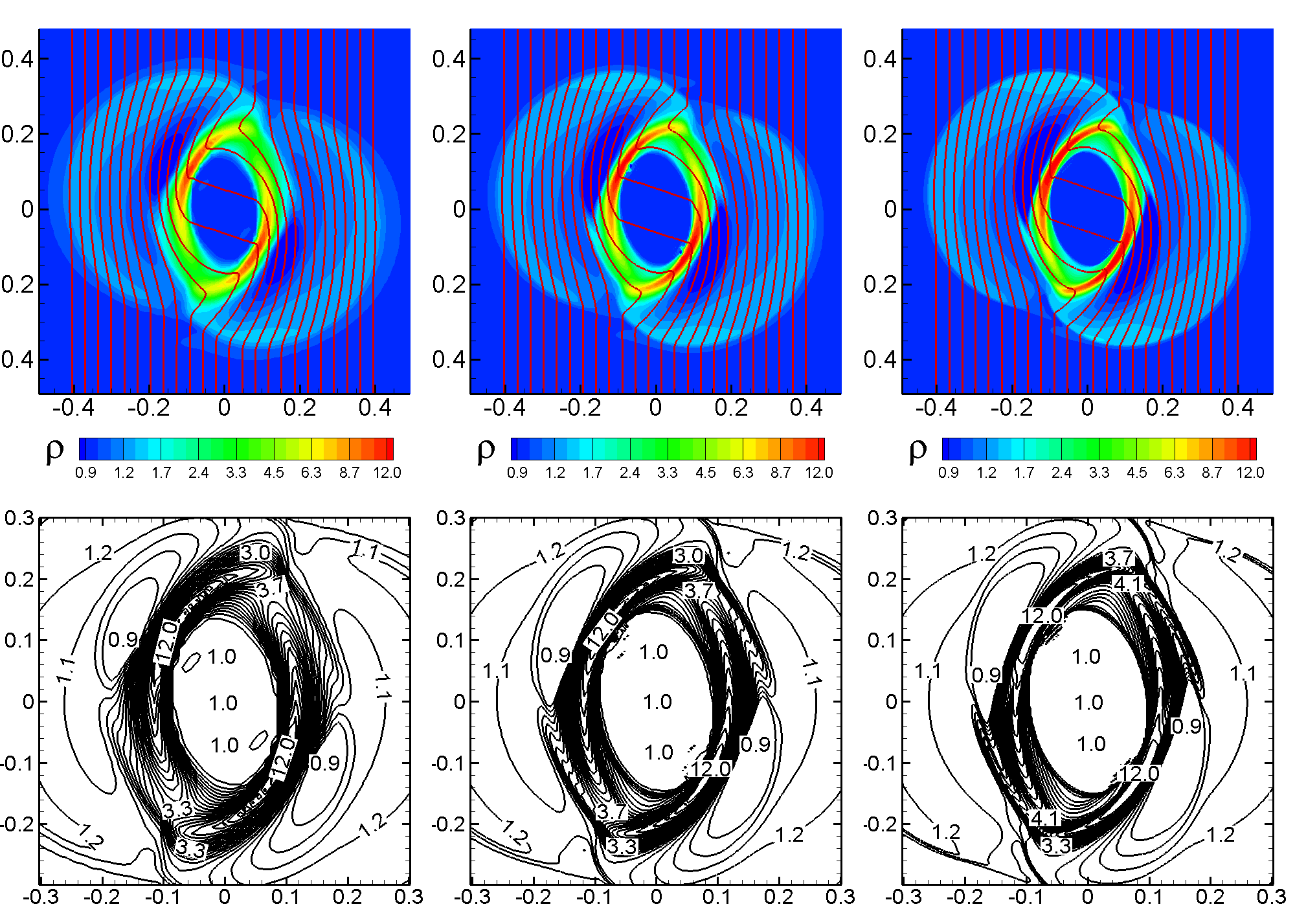
Figure 26: Test of the ideal MHD block of the code with the “rotor problem” test at different grid resolutions. Top Panels: Density distribution (color background) and field lines (solid lines) with grid resolution $100\times 100$ (left panel), $200\times 200$ (middle panel) and $400\times 400$ (right panel). Bottom Panels: The density contour lines.

C.1 Test of the ideal MHD block

To check the MHD block of the code we performed the standard “rotor problem” test. This test has been used by a number of authors for testing MHD solvers including the energy equation (e.g., Balsara & Spicer 1999). We use this test to check our ideal MHD block of the code (viscosity and diffusivity are switched off) with an isentropic equation $dS/dt=0$ instead of the energy equation. In this situation the shock waves do not have physical sense. However, the goal of this test is not to test the physics of shock waves, but instead to demonstrate the ability of the numerical algorithm to solve the 2D adiabatic MHD equations.

We solve the MHD equations numerically in the region $-0.5<x<0.5$, $-0.5<y<0.5$ in a Cartesian geometry. At the beginning of simulations, $t=0$, the pressure in the region is constant, $p=1$, and the magnetic field is homogeneous, $B_{x}=0$, $B_{y}=5$. In the center there is a circle with radius $r_{0}=0.1$ (radius $r=\sqrt{x^{2}+y^{2}}$) where the density of matter is $\rho_{0}=10$ and the matter rotates as a solid body with angular velocity $\omega_{0}=20$. At $r>r_{1}=0.115$, the density is $\rho_{1}=1$ and the matter is at rest. In the ring $r_{0}<r<r_{1}$, the density and velocity are linearly interpolated between those at $r=r_{0}$ and $r=r_{1}$.

The equations of ideal adiabatic MHD were solved with the Godunov-type scheme used in the “main” code. In the test we used a homogeneous grid with step $\Delta x=\Delta y=1/N$, where $N=100,200,400$. The time-step is chosen from the condition $\Delta t=0.4\Delta x/v_{max}$, where $v_{max}$ is the maximum velocity of propagation of the perturbations. The results of the simulations are shown in Fig. 26. One can see that the density and the field line distribution is very similar in all three cases, while simulations at the highest grid resolutions give almost identical results and the convergence of the results is evident. The bottom panels of Fig. 26 show selected streamlines with numbers which confirm the similarity and convergence of the results. The test had been performed on a homogeneous grid, while our simulations were done in spherical coordinates with a high grid resolution near the star, and much coarser resolution at the outer boundary of the simulation region. In this paper we mainly investigate the launching of jets and winds from the disk, and therefore we need to have adequate grid resolution in the region where matter is launched from the disk into the winds, that is, at radii $r\approx 2-3$ for the conical winds, and $r\approx 3-5$ for the propeller-driven winds. The grid resolution at these radii corresponds approximately to the homogeneous grid with the lowest grid resolution, $100\times 100$. The above test shows that the grid resolution in this region is sufficiently good for investigation of the physics of outflows in this region. It is clear that the grid resolution at larger distances, and in particular close to the outer boundary is not very high. However, this region does not influence the physics of the process. In this region matter flows either inward due to the viscosity (in the disk), or outward as winds (in the corona). We expect larger simulation errors in these regions, but these do not change the main result: the launching of winds from the disk-magnetosphere boundary. The magnetic force accelerating matter into the jet component has higher accuracy close to the star and less accuracy at larger distances. However, Fig. 11d shows that the main acceleration into the wind occurs close to the star where the grid resolution is good.

We are planning future simulations with higher resolutions and in larger regions with the recently MPI-parallelized version of our code.

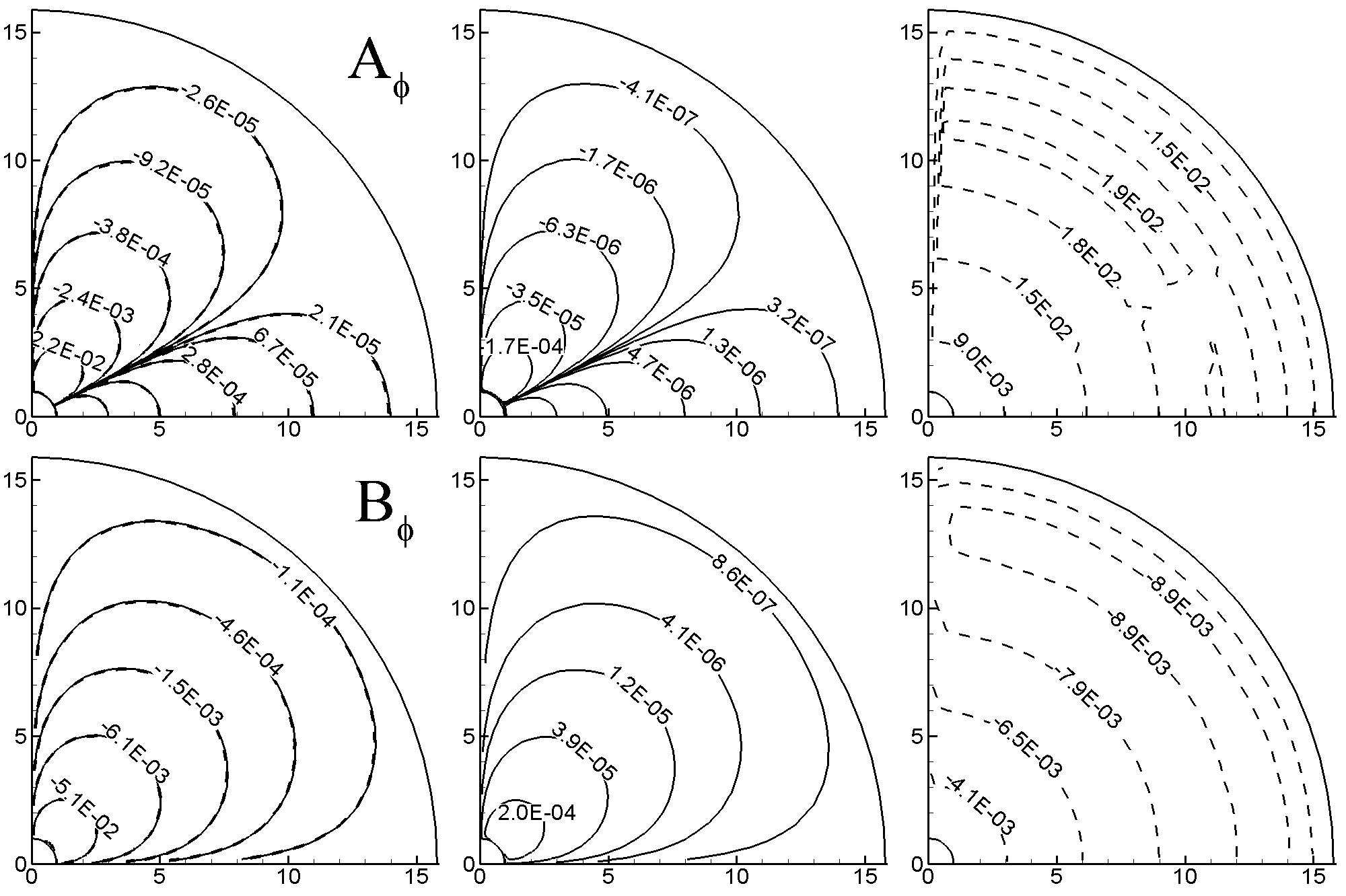
Figure 27: Test of the diffusivity block of the code on the grid $51\times 31$. The top panels show analysis of the vector-potential, $A_{\phi}$. The left hand panel shows the simulated value $A_{\phi}^{num}$ (solid lines) and the exact solution $A_{\phi}^{exact}$ (dashed lines). The middle panel shows the absolute error $\Delta A_{\phi}=A_{\phi}^{num}-A_{\phi}^{exact}$, and the right hand panel shows the relative error, $\Delta A_{\phi}/A_{\phi}^{exact}$. The bottom panels show similar analysis but for the azimuthal component of the magnetic field, $B_{\phi}$.

	Grids	$\max|\Delta A_{\phi}|$	$\max|\Delta B_{\phi}|$
$51\times 31$		$1.32\times 10^{-3}$	$7.11\times 10^{-4}$
$75\times 45$		$6.20\times 10^{-4}$	$3.24\times 10^{-4}$
$101\times 61$		$3.40\times 10^{-4}$	$1.75\times 10^{-4}$

Table 2: The maximum absolute error in calculations of the $A_{\phi}$ and $B_{\phi}$ obtained in the diffusivity tests at different grid resolutions.

C.2 Test of the diffusivity block

Here we test the diffusivity block of the code. For this we “switch off” the hydrodynamic fluxes and the corresponding right-hand side terms in equations A5 and A6 and integrate these equations numerically in the region $r_{0}<r<r_{1}$, $0<\theta<\pi/2$. In the case of the constant diffusivity coefficient (we take $\eta=1$) equations A5 and A6 coincide, and so the problems for the azimuthal component of the vector-potential and for the azimuthal magnetic field differ only in the boundary conditions at the equator (at $\theta=\pi/2$) and the initial conditions. That is,

$$\frac{\partial{A_{\phi}}}{\partial{\theta}}{\bigg{|}}_{\theta=\pi/2}=0,~{}~{}B_{\phi}{\bigg{|}}_{\theta=\pi/2}=0.$$

On the symmetry axis ($\theta=0$) we have:

$$A_{\phi}|_{\theta=0}=0,~{}~{}B_{\phi}|_{\theta=0}=0.$$

We can find some particular solutions of equations (A5) and (A6) by the separation of variables method. For testing we choose the following solutions:

$$A_{\phi}=\frac{C\sin\theta}{r^{2}}\bigg{(}1-\frac{5\sin 2\theta}{4}\bigg{)}\bigg{(}1+\frac{10\eta(t_{0}-t)}{r^{2}}\bigg{)},$$ (17)

$$B_{\phi}=\frac{C\sin\theta\cos\theta}{r}\bigg{(}1+\frac{6\eta(t_{0}-t)}{r^{2}}\bigg{)},$$ (18)

where $C$ and $t_{0}$ are constants. Equations for the $\phi$-components of the vector-potential and magnetic field were integrated numerically using our 2.5D code (with the “switched-off” hydro fluxes and zero right-hand-side terms). We used the same grid geometry as in the main simulations; that is, spherical coordinates with an equidistant grid in the meridional direction and expanding grid in the radial direction, where the expansion factor is determined by the fact that we keep all sides of each grid cell to be approximately equal. For the test we used the grid corresponding to the main simulation runs in the conical wind, $N_{r}=51$ and $N_{\theta}=31$, and also we used finer grids, $75\times 45$ and $101\times 61$. We took the inner and outer radii of the simulation region to be the same as in the conical wind case, $r_{0}=1$, $r_{1}=15.9$. For these boundaries we set $A_{\phi}$ and $B_{\phi}$ to be equal to the analytical values determined by equations 17 and 18. The initial conditions corresponded to the exact solutions (17 and 18) at $t=0$.

The constants $C$ and $t_{0}$ in 17 and 18 were chosen so that the solutions at the inner boundary are of the order of unity. We used $C=0.01$, $t_{0}=50$. We integrated the equations up to $t_{1}=2t_{0}=100$.

Fig. 27 (top panels) shows the result of the diffusivity test for the vector-potential, $A_{\phi}$. The solid line in the left panel shows the numerical solution, $A_{\phi}^{num}$, which is obtained by integrating equation A5, at time $t=100$. The dashed line shows the exact solution, $A_{\phi}^{exact}$, obtained by integrating the exact solution 17. One can see that the solutions are very close to each other, and the dashed line is barely visible. The middle panel shows the absolute error $\Delta A_{\phi}={A_{\phi}^{num}-A_{\phi}^{exact}}$. One can see that the error is very small everywhere, taking into account the fact that the maximum value of the function, $A_{\phi}\approx 1$. The error increases towards the star. However, this is because the value of the function $A_{\phi}$ strongly increases towards the star. The right hand panel shows that the relative error, $(A_{\phi}^{num}-A_{\phi}^{exact})/A_{\phi}^{exact}$, decreases towards the star. One can see that the relative error in calculation of the diffusivity is also small and is of the order of $(1-2)\%$. Fig. 27 (bottom panels) shows similar analysis for the $B_{\phi}$ component, where equations (A6) and 18 have been solved for the numerical and exact solutions.

We performed similar simulations and analysis at finer grid resolutions, $75\times 45$ and $101\times 61$. Table 2 shows the maximum absolute error, $\max{|A_{\phi}^{num}-A_{\phi}^{exact}|}$. One can see that at the finer grids, $75\times 45$ and $101\times 61$, this error is $2.1$ and $3.9$ times smaller compared to the coarsest grid, $51\times 31$. This confirms the convergence of the numerical solution towards the analytical solution. Similar comparisons for the $B_{\phi}$ component give factors $2.2$ and $4.1$, which also show convergence.

A complete description of our methods and tests will be given in a separate paper.

Appendix D Parameter ranges of conical winds

To investigate the dependence on different parameters we took the main case and varied one parameter at a time. We performed several sets of runs: (1) with a fixed diffusivity and different viscosity coefficients; (2) with a fixed viscosity and different diffusivity coefficients; (3) with different rotation periods of the star $P_{*}$; (4) with different coronal densities.

D.1 Dependence on viscosity at fixed diffusivity

We fixed the diffusivity at $\alpha_{d}=0.1$ and varied the viscosity coefficient in the range $\alpha_{v}=0.01-1$. Fig. 28 shows matter fluxes onto the star and into the conical winds through the surface $r=6$. We observed that for small viscosity, $\alpha_{v}<0.1$, the magnetic field of the dipole diffuses through the inner regions of the incoming disk and an X-type configuration does not form. No conical winds appear in this case. We conclude that formation of conical winds requires $\alpha_{v}\gtrsim\alpha_{d}$, that is, Pr${}_{m}\gtrsim 1$. Next we increased $\alpha_{v}$ and observed that an X-type configuration formed and conical winds were generated. We observed that the accretion rate to the star increases with $\alpha_{v}$, while the mass outflow rate into the conical winds increases but only slowly. For $\alpha_{v}=0.1$, the matter fluxes onto the star and into the wind are small and approximately equal. For $\alpha_{v}=0.3$ and $\alpha_{v}=0.4$, the wind carries about $30\%$ and $20\%$ of mass respectively. The angular momentum carried to the star also strongly increases with $\alpha_{v}$. In all cases the star spins up, because the magnetospheric radius, $r_{m}\approx 1.2$ is smaller than corotation radius $r_{cor}=3$. That is, the incoming matter brings positive angular momentum onto the star. The conical wind carries angular momentum away from the disk. Notice, however, that this is only a small part of the total angular momentum of the disk as shown above.

Figure 28: Matter and angular momentum fluxes onto the star and into the wind for fixed diffusivity $\alpha_{d}=0.1$ but different coefficients of viscosity, $\alpha_{v}$.

Figure 29: Matter and angular momentum fluxes onto the star and into the wind for fixed viscosity $\alpha_{v}=0.3$ but different coefficients of diffusivity, $\alpha_{d}$.

D.2 Dependence on diffusivity at fixed viscosity

In the next set of runs we fixed the viscosity at $\alpha_{v}=0.3$ and varied the diffusivity: from 0.01 to 1. Fig. 29 shows the integrated matter fluxes onto the star and into the wind at different diffusivities. We observed that no conical winds were formed for $\alpha_{d}\gtrsim\alpha_{v}$. At relatively high diffusivity, $\alpha_{d}=0.1,~{}0.3$, about $30\%$ of the incoming matter flows into the conical wind. For $\alpha_{d}=0.1$ (Pr${}_{m}=3$), the matter flux into the conical wind oscillates, while at $\alpha_{d}=0.3$ (Pr${}_{m}=1$) no oscillations are observed. The conical wind also forms for very small diffusivity, $\alpha_{d}=0.01$, but with slightly smaller matter flux into the wind. Angular momentum fluxes to the star and into the winds are approximately the same, excluding the case $\alpha_{d}=0.01$ where the flux to the star is larger.

D.3 Variation of star’s period

We varied the period of the star (via the corotation radius) taking $r_{cor}=3,~{}10$ for slowly rotating stars and $r_{cor}=1.0,~{}1.5,~{}2$ for more rapidly rotating stars. In the case of very slow rotation, $r_{cor}=10$, conical winds form and the outflow rate into the wind is similar to that in the main case ($r_{cor}=3$), although the accretion rate onto the star is somewhat larger. In stars with higher spin, $r_{cor}=2$, the amplitude of variability increases and the matter flux into the outflows increases up to $50\%$ of the accretion rate to the star. For even higher spin, $r_{cor}=1.5$, the accretion rate to the star decreases by a factor of $5$ compared with the main case, while the outflow rate into the conical wind strongly increases. Thus when a star rotates more rapidly, the winds become more powerful, and the accretion rate to the star decreases, and therefore the situation becomes closer to the propeller regime. In rapidly rotating stars, the outbursts become episodic, and the interval between outbursts increases with spin. In addition, the volume occupied by the fast coronal component increases with spin: at $r_{cor}=10$ there is no fast component in the corona, at $r_{cor}=3$ it occupies some region above the conical winds (see Fig. 7a), while at $r_{cor}=2$ it occupies a much larger region (see Fig. 7b). At even higher spin this region occupies the whole simulation region as in the propeller regime.

D.4 Variation of coronal density

Outflow of matter into a wind occurs if the corona is not very dense, and hence outflowing matter of the winds does not lose its energy while propagating through the corona. In the main simulation runs the initial density of the corona is $10^{4}$ times lower compared to the disk density ( $\rho_{c}=10^{-3}$ versus $\rho_{d}=10$). To test the dependence on the coronal density we decreased its density by a factor of $3$. These simulations showed that the matter fluxes onto the star and into the winds are not appreciably different from the main case. We conclude that the coronal density used in the main case is sufficiently small not to affect the outflows.

The situation is different in the coronal region. For slowly rotating stars (the conical wind regime) there are no forces which tend to drive matter along the axis. Fast flow appears only in the part of corona where the stellar field lines are strongly inclined (see Fig. 3, Fig. 7). The rest of the corona has very slow motion towards or away from the star. The top half of the coronal region is matter-dominated (Fig. 13a,d) and might be an obstacle to a fast outflow. We suggest that at lower coronal density the fast coronal component might occupy a larger region.

In the propeller regime where the star rotates rapidly, the magnetic force is larger and drives the low-density coronal matter into the fast jet. The corona is magnetically-dominated (see Fig. 16a,d) during the whole simulation time. Initially, the density in the corona $\rho_{c}=10^{-4}$ is $10$ times lower than in case of slowly rotating stars. However, the initial density distribution is important only at the beginning of the long simulation runs. Later the density distribution is established by the outflow process. The main process is inflation of the dipole field lines. Inflating field lines carry matter along both disk and stellar field lines, and as a result, some matter penetrates into the corona. Strong disk oscillations and violent processes of inflation during which the conical wind component often changes its opening angle) lead to the penetration of a small amount of matter into the corona. The density increases away from the axis, where it is very small, towards the conical wind. In the case of a slowly rotating star, the disk oscillations are weaker and there are no violent inflation events. For this reason the axial region above the star has a very low density.

References

- (1) Alencar, S. H. P., Basri, G., Hartmann, L., Calvet, N. 2005 A&A, 440, 595
- (2) Alpar, M.A., & Shaham, J. 1985, Nature, 316, 239
- (3) Aly, J.J., & Kuijpers, J. 1990, A&A, 227, 473
- (4) Bacciotti, F., Mundt, R., Ray, T.P., Eisl ffel, J., Solf, J., Camezind, M. 2000, ApJ, 537, L49
- (5) Balsara, D.S., & Spicer, D.S. 1999, J. Comp. Phys., 149, 1999, 270
- (6) Berger, E., Rutledge, R.E., Phan-Bao, N., Basri, G. et al. 2009, ApJ, 695, 310
- (7) Bessolaz, N., Zanni, C., Ferreira, J., Keppens, R., Bouvier, J. 2008, A&A, 478, 155
- (8) Bisnovatyi-Kogan, G.S., & Lovelace, R.V.E. 2007, ApJ, 667, L167
- (9) Blandford, R.D., & Payne, D.G. 1982, MNRAS, 199, 883
- (10) Boutloukos S., van der Klis M., Altamirano D., Klein-Wolt M., Wijnands R., Jonker P.G., Fender R.P., 2006, ApJ, 653, 1435
- (11) Bouvier, J., Alencar, S. H. P., Boutelier, T., Dougados, C., Balog, Z., Grankin, K., Hodgkin, S. T., Ibrahimov, M. A., Kun, M., Magakian, T. Yu., & Pinte, C. 2007, A&A, 463, 1017
- (12) Brittain, S., Simon, T., Rettig, T.W., et al. 2007, Star-Disk Interaction in Young Stars, IAU Symposium No. 243, ed. J. Bouvier & I. Appenzeller, p. 223
- (13) Brio, M., & Wu, C.C. 1988, Computat. Phys., 75, 400
- (14) Cabrit, S., Edwards, S., Strom, S.E., & Strom, K.M. 1990, ApJ, 354, 687
- (15) Cai, M.J., Shang, H., Lin, H.-H., & Shu, F.H. 2008, ApJ, 672, 489
- (16) Casse, F., & Keppens, R. 2004, ApJ, 601, 90
- (17) Chabrier, G., Baraffe, I., Selsis, F., Barman, T. S., Hennebelle, P., Alibert, Y. 2007, Protostars and Planets V, B. Reipurth, D. Jewitt, and K. Keil (eds.), University of Arizona Press, Tucson, 951 pp., 2007., p.623-638
- (18) Coffey, D., Downes, T. P., & Ray, T. P. 2004, A&A, 419, 593
- (19) Cooke, R., Bland-Hawthorn, J., Sharp, R., & Kuncic, Z. 2008, ApJ, 687, L29
- (20) Cranmer, S. 2008, ApJ, 689, 316
- (21) Donati, J.-F., Forveille, T., Cameron, A.C., Barnes, J.R., Delfosse, X., Jardine, M.M., & Valenti, J.A. 2006, Science, 311, 633
- (22) Dupree, A.K., Brickhouse, N.S., Smith, G.H., & Strader, J. 2005, ApJ 625, L131
- (23) Edwards, S., Fischer, W., Hillenbrand, L., Kwan, J. 2006, ApJ, 646, 319
- (24) Edwards, S., Fischer, W., Kwan, J., Hillenbrandt, L., Durpee, A.K. 2003, ApJ, 599, L41
- (25) Edwards, S. 2009, Proceedings of the 15th Cambridge Workshop on Cool Stars, Stellar Systems and the Sun. AIP Conference Proceedings, Volume 1094, pp. 29-38
- (26) Fendt, C. 2009, ApJ, 692, 346
- (27) Fendt, C., & Elstner, D. 2000, A&A, 363, 208
- (28) Fendt, C., & Cemeljić, M. 2002, A&A, 395, 1045
- (29) Ferreira, J, Dougados, C., & Cabrit, S. 2006, A&A, 453, 785
- (30) Fomalont, E. B., Geldzahler, B. J., & Bradshaw, C. F. 2001, ApJ, 553, L27
- (31) Frank, A., & Mellema, G. 1996, ApJ, 472, 684
- (32) Ghosh, P., & Lamb, F.K. 1979, ApJ, 234, 296
- (33) Goodson, A.P., & Winglee, R. M., 1999, ApJ, 524, 159
- (34) Goodson, A.P., Winglee, R. M., & Böhm, K.-H. 1997, ApJ, 489, 199
- (35) Goodson, A.P., Böhm, K.-H., Winglee, R. M. 1999, ApJ, 524, 142
- (36) Hartigan, P, Edwards, S., & Gandhour, L. 1995, ApJ, 452, 736
- (37) Hayashi, M. R., Shibata, K., & Matsumoto, R. 1996, 468, L37
- (38) Heinz, S., Schulz, N. S., Brandt, W. N., & Galloway, D. K. 2007, ApJ, 663, L93
- (39) Herbst, W., Herbst, D. K., Grossman, E. J., Weinstein, D. 2004, AJ, 108, 1906
- (40) Hirose, S., Uchida, Yu., Shibata, K., & Matsumoto, R. 1997, PASJ, 49, 193
- (41) Iaria R., D’Aí A, Lavagetto G., Di Salvo T., Robba N.R., Burderi L., 2008, ApJ, 673, 1033
- (42) Igumenshchev, I. V., Narayan, R., & Abramowicz, M. A. 2003, ApJ, 592, 1042
- (43) Igumenshchev, I.V. 2008 ApJ, 677, 317
- (44) Illarionov, A.F., & Sunyaev, R.A. 1975, A&A, 39, 185
- (45) Jonker, P.G., Nelemans, G., Bassa, C.G. 2007, MNRAS, 374, 999
- (46) Kershaw D.S. 1978, J. Comp. Phys., 26, 43
- (47) Koldoba, A. V., Romanova, M. M., Ustyugova, G. V., & Lovelace, R. V. E. 2002, ApJ, 576, L53
- (48) Koldoba, A. V., Ustyugova, G. V., Romanova, M. M., & Lovelace, R. V. E. 2008, MNRAS, 388, 357
- (49) Königl, A., & Pudritz, R. E. 2000, Protostars and Planets IV, Mannings, V., Boss, A.P., Russell, S. S. (eds.), University of Arizona Press, Tucson, p. 759
- (50) Krasnopolsky, R., Li, Z.-Y., & Blandford, R.D. 1999, ApJ, 526, 631
- (51) Krist, J.E. et al. 2008, ApJ, 136, 1980
- (52) Küker, M., Henning, T., & Rüdiger, G. 2003, ApJ, 589, 397
- (53) Kulkarni, A., & Romanova, M.M. 2008, MNRAS, 386, 673
- (54) Kulkarni, A., & Romanova, M.M. 2009, MNRAS, submitted (arXiv:0812.0241)
- (55) Kulikovskii, A. G., Pogorelov, N. V., & Semenov, A. Y. 2001, Mathematical Aspects of Numerical Solution of Hyperbolic Systems (Boca Raton: Chapman & Hall)
- (56) Kwan, J., Edwards, S., & Fischer, W. 2007, ApJ, 657, 897
- (57) Lamzin, S.A. 1998, Astronomy Report, 42, 322
- (58) Li, H., Finn, J.M., Lovelace, R.V.E., & Colgate, S.A. 2000, ApJ, 533, 1023
- (59) Livio, M. 1997, Accretion Phenomena and Related Outflows; IAU Colloquium 163. ASP Conference Series; Vol. 121; ed. D. T. Wickramasinghe; G. V. Bicknell; and L. Ferrario, p.845
- (60) Long, M., Romanova, M. M., & Lovelace, R. V. E. 2005, ApJ, 634, 1214
- (61) ——— 2007, MNRAS, 374, 436
- (62) ——— 2008, MNRAS, 386, 1274
- (63) Lovelace, R.V.E., Mehanian, C., Mobarry, C.M., & Sulkanen, M.E. 1986, ApJ, 62, 1
- (64) Lovelace, R.V.E., Berk, H.L., & Contopoulos, J. 1991, ApJ, 379, 696
- (65) Lovelace, R.V.E., Li, H., Colgate, S.A., & Nelson, A.F. 1999, ApJ, 513, 805
- (66) Lovelace, R.V.E., Romanova, M.M., & Bisnovatyi-Kogan, G.S. 1995, MNRAS, 275, 244
- (67) Lovelace, R.V.E., Romanova, M.M., & Bisnovatyi-Kogan, G.S. 1999, ApJ, 514, 368
- (68) Lovelace, R.V.E., Romanova, M.M., & Newman, W.I. 1994, ApJ, 437, 136
- (69) Lovelace, R.V.E., Li, H., Koldoba, A.V., Ustyugova, G.V., & Romanova, M.M. 2002, ApJ, 572, 445
- (70) Lorenzetti, D., Giannini, T., Calzoletti, L., Puccetti, S., Antoniucci, S., Arkharov, A. A., di Paola, A., Larionov, V. M., Nisini, B. 2006, A&A, 453, 579
- (71) Matsakos, T., Tsinganos, K., Vlahakis, N., Massaglia, S., Mignone, A., Trussoni, E. 2008, A&A, 477, 521
- (72) Matt, S., Goodson, A.P., Winglee, R.M., & Böhm, K.-H. 2002, ApJ, 574, 232
- (73) Matt, S., Winglee, R.M., & Böhm, K.-H. 2003, MNRAS, 345, 660
- (74) Matt, S., & Pudritz, R.E. 2005, ApJ, 632, 135
- (75) Matt, S., & Pudritz, R.E. 2008, ApJ, 681, 391
- (76) Meier, D.L. 2005, Ap&SS, 300, 55
- (77) Miller, K.A., & Stone, J.M. 1997, ApJ, 489, 890
- (78) Moffat, H.K. 1978, Magnetic Field Generation in Electrically Conducting Fluids (Cambridge: Cambridge University Press)
- (79) Mohanty, S., Jayawardhana, R., & Basri, G. 2005, ApJ, 626, 498
- (80) Mohanty, S., & Shu, F.H. 2008, ApJ, 687, 1323
- (81) Murdin P., Jauncey D.L., Haynes R.F., Lerche I., Nicolson G.D., Holt S.S., Kaluzienski L.J., 1980, A&A, 87, 292
- (82) Najita, J.R., & Shu, F.H. 1994, ApJ, 429, 808
- (83) Nisini, B., Antoniucci, S., Giannini, T., & Lorenzetti, D. 2005, A&A, 429, 543
- (84) Natta, A., Testi, L., Muzerolle, J., Randich, S., Comerón, F., & Persi, P. 2004, A&A, 424, 603
- (85) Ostriker, E.C., & Shu, F.H. 1995, ApJ, 447, 813
- (86) Pyo, T.-S., Hayashi, M., Kobayashi, N. et al. 2003, ApJ, 649, 836
- (87) Pyo, T.-S., Hayashi, M., Kobayashi, N. et al. 2006, ApJ, 649, 836
- (88) Reiners, A., Basri, G., & Christensen, U.R. 2009, ApJ, in press (arXiv:0903.0857)
- (89) Ray, T., Dougados, C., Bacciotti, F., Eisl ffel, J., & Chrysostomou, A. 2007, Protostars and Planets V, B. Reipurth, D. Jewitt, and K. Keil (eds.), University of Arizona Press, Tucson, p. 231
- (90) Romanova, M.M., Kulkarni, A.K., & Lovelace, R.V.E. 2008, ApJ, 673, L171
- (91) Romanova, M.M., Ustyugova, G.V., Koldoba, A.V., & Lovelace, R.V.E. 1997, ApJ, 482, 708
- (92) Romanova, M.M., Ustyugova, G.V., Koldoba, A.V., & Lovelace, R.V.E. 2002, ApJ, 578, 420 (R02)
- (93) Romanova, M.M., Ustyugova, G.V., Koldoba, A.V., Wick, J.V., & Lovelace, R.V.E. 2003, ApJ, 595, 1009
- (94) Romanova, M.M., Ustyugova, G.V., Koldoba, A.V., & Lovelace, R.V.E. 2004a, ApJ, 616, 151L
- (95) Romanova, M.M., Ustyugova, G.V., Koldoba, A.V., & Lovelace, R.V.E. 2004b, ApJ, 610, 920
- (96) Romanova, M.M., Ustyugova, G.V., Koldoba, A.V., & Lovelace, R.V.E. 2005, ApJ, 635, 165L (R05)
- (97) Romanova, M.M., Long, M., Kulkarni, A. K., Kurosawa, R., Ustyugova, G.V., Koldoba, A.K., & Lovelace, R.V.E. 2007, in IAU Symp., Vol. 243, Star-Disk Interaction in Young Stars, ed. J. Bouvier & I. Appenzeller
- (98) Romanova, M.M., Ustyugova, G.V., Koldoba, A.V., & Lovelace, R.V.E. 2008, in “Protostellar Jets in Context”, editors: profs. Tom Ray and Kanaris Tsinganos, arXiv:0901.3858
- (99) Rothstein, D.M., & Lovelace, R.V.E. 2008, ApJ, 677, 1221
- (100) Scholz, A., Jayawardhana, R., & Brandeker A 2005, ApJ, 629, L41
- (101) Shakura, N.I., & Sunyaev, R.A. 1973, A&A, 24, 337
- (102) Shibata, K., & Uchida, Y. 1985, PASJ, 37, 31
- (103) Shu, F., Najita, J., Ostriker, E., Wilkin, F., Ruden, S., Lizano, S. 1994, ApJ, 429, 781
- (104) Shu, F.H, Galli, D., Lizano, S., Glassgold, A.E., & Diamond, P.H. 2007, ApJ, 665, 535
- (105) Sokoloski, J.L. 2003, JAVSO, 31, 89
- (106) Sokoloski, J.L., & Bildsten, L. 1999, ApJ, 517, 919
- (107) Sokoloski, J.L., Bildsten, L., & Ho, W. 2001, MNRAS, 326, 553
- (108) Spruit, H. C., & Taam, R. E. 1990, A&A, 229, 475
- (109) Stone, J. M., Gammie, C. F., Balbus, S. A., & Hawley, J. F. 2000, Protostars and Planets IV (Book - Tucson: University of Arizona Press; eds Mannings, V., Boss, A.P., Russell, S. S.), p. 589
- (110) Takami, M., Beck, T.L., Pyo,T.-S., McGregor, P., Davis, C. 2007, ApJ, 670, L33
- (111) Toth, G. 2000, Computat. Phys., 161, 605
- (112) Tudose, V., Fender, R. P., Tzioumis, A. K., Spencer, R. E., & van der Klis, M. 2008, MNRAS, 390, 447
- (113) von Rekowski, B., & Brandenburg, A. 2004, A & A, 420, 17
- (114) Uchida, Y., & Shibata, K. 1985, PASJ, 37, 515
- (115) Ustyugova, G.V., Koldoba, A.V., Romanova, M.M., & Lovelace, R.V.E. 1999, ApJ, 516, 221
- (116) Ustyugova, G.V., Lovelace, R.V.E., Romanova, M.M., Li, H., & Colgate, S.A. 2000, ApJ, 541, L21
- (117) Ustyugova, G.V., Koldoba, A.V., Romanova, M.M., & Lovelace, R.V.E. 2006, ApJ, 646, 304 (U06)
- (118) Uzdensky, D.A. 2002, ApJ, 572, 432
- (119) Whelan, E.T., Ray, T.P., & Bacciotti, F. 2009, ApJ, 691, L106
- (120) Yelenina, T. G., Ustyugova, G. V., & Koldoba, A. V. 2006, A&A, 458, 679