Quantum key distribution using vacuum-one-photon qubits: maximum number of transferable bits per particle

Abstract

Quantum key distribution schemes which employ encoding on vacuum-one-photon qubits are capable of transferring more information bits per particle than the standard schemes employing polarization or phase coding. We calculate the maximum number of classical bits per particle that can be securely transferred when the key distribution is performed with the BB84 and B92 protocols, respectively, using the vacuum-one-photon qubits. In particular, we show that for a generalized B92 protocol with the vacuum-one-photon qubits, a maximum of two bits per particle can be securely transferred. We also demonstrate the advantage brought about by performing a generalized measurement that is optimized for unambiguous discrimination of the encoded states: the parameter range where the transfer of two bits per particle can be achieved is dramatically enhanced as compared to the corresponding parameter range of projective measurements.

1 Introduction

Quantum key distribution (QKD), as first suggested by Bennett and Brassard [1], provides a way for two parties, known as Alice and Bob, to share a key with secrecy guaranteed by the laws of quantum physics. Since its first demonstration in 1992 [2], QKD has been extensively studied both theoretically and experimentally to the point that it now represents probably the most advanced application of quantum information processing [3]. In most current QKD implementations, information is encoded either in polarization or in phase of individual photons. The popularity of the polarization and phase codings stems from the fact that it is relatively easy and straightforward to manipulate the polarization and phase of photons with the already-existing optics technology.

Another possibility for the implementation of QKD protocols is “photon-number coding” in which information is encoded on vacuum-one-photon qubits (VOPQs). By a VOPQ we mean a qubit for which the two basis states are $|0\rangle$, the vacuum state, and $|1\rangle$, the one-photon state. In contrast to the QKD schemes employing polarization or phase coding in which the signal is carried by individual photons, QKD schemes with VOPQs utilize pulses in superpositions of the vacuum and one-photon states as the signal carrier. QKD schemes with VOPQs suffer from an obvious practical disadvantage that it is generally difficult to generate and detect such superpositions. Nevertheless, recent theoretical and experimental progress in the generation and detection of arbitrary superpositions of the vacuum and one-photon states using techniques of linear optics [4, 5, 6, 7, 8, 9, 10] and cavity QED [11, 12, 13], respectively, appears to open up avenues for quantum information processing with VOPQs. In particular, quantum teleportation with VOPQs has been studied theoretically [14, 15, 16, 17, 18] and demonstrated experimentally [19, 20]. QKD schemes based on vacuum-one-photon entangled states (single-photon entangled state [14, 21]) have also been considered very recently [22, 23]. Another practical disadvantage of QKD schemes with VOPQs is that photon losses which are inevitable lead not just to reduced key rates but also to errors caused by misidentification of the one-photon state with the vacuum state. This limits the photon loss rate and consequently the distance over which the key can be distributed.

In this work we study the BB84 [1] and B92 [24] QKD schemes using vacuum-one-photon qubits, exploiting in particular the interesting property of the VOPQ, already noted earlier [8], that it allows for low-energy-expense encoding of quantum information, as it requires, on average, less than one photon for each qubit. The number of photons that Alice needs to send to Bob in order to transfer a given amount of information can therefore be smaller with VOPQs than with other qubit systems. This “cost effectiveness” of the QKD scheme employing VOPQs is a practically important characteristic that makes it worthwhile to study.

The paper is organized as follows. Sec. 2 introduces the parameters that quantify the cost effectiveness of QKD schemes. In Sec. 3 we first discuss the cost effectiveness of the BB84 protocol and then in detail that of the B92 protocol. We first deal with the case when the encoding states are detected using standard quantum measurements (Projector Valued Measurements, PVMs). The central result of the paper is that optimal cost effectiveness can be realized in a much larger range of the parameters if an optimized generalized measurement (a Positive Operator Valued Measurement, POVM) is employed for the detection of the encoding states. In Sec. 4 and 5, respectively, we discuss effects of photon losses and of eavesdropping attacks on QKD schemes using VOPQs. Finally, Sec. 6 presents discussion and summary of our main findings.

2 Effectiveness parameters

The problem of the cost effectiveness of a QKD scheme that we deal with here is closely related to one of the most fundamental issues in information theory, namely, how efficiently information can be transmitted from input to output of a communication channel. The classical theory due to Shannon [25] states that the amount of information that can be transmitted is limited by the Shannon entropy, a statistical measure of information per “letter” of input. In quantum communication, which deals with quantum channels (quantum systems operating as communication channels) transmitting signals that are prepared at the input in the form of quantum states and measured at the output via quantum state measurements, it is the von Neumann entropy that limits the amount of information transmitted [26, 27]. Thus, when information is carried by qubits, the maximum information per qubit that can be transmitted is one bit, which is referred to as the Holevo limit [28, 29]. The issue we address in this paper has to do with the transmission efficiency of a QKD scheme, i.e., we study the question of what are the maximum bits of information per qubit and per photon, repectively, that can be securely transferred from Alice to Bob, while preventing an eavesdropper, Eve, from acquiring information without being detected. A similar issue has recently been investigated by Cabello [30].

For a quantitative discussion of the cost effectiveness of a QKD scheme, we first define the “qubit effectiveness parameter” H as

$$H=\frac{n_{b}}{n_{q}}\ ,$$ (1)

where $n_{q}$ is the number of qubits sent from Alice to Bob, and $n_{b}$ represents the number of classical information bits that are securely transferred from Alice to Bob. This parameter H, which gives the ratio of the length of the sifted key to the length of the raw key, may be considered to measure the degree of effectiveness with which a given QKD protocol produces a secretly shared key per qubit sent. The Holevo limit establishes an upper bound to H, i.e.,

$$H\leq 1\ .$$ (2)

Another parameter of interest that we wish to consider is the “particle effectiveness parameter” or the “cost effectiveness parameter” K defined as

$$K=\frac{n_{b}}{n_{p}}\ ,$$ (3)

where $n_{p}$ is the number of particles (photons) sent from Alice to Bob. In standard QKD schemes employing polarization or phase coding, $n_{p}$ and $n_{q}$ are the same and thus $K=H$. When QKD schemes with VOPQs are considered, however, $n_{p}\leq n_{q}$ and thus $K\geq H$. We note that the vacuum plays the role of a part of the signal in the QKD schemes with VOPQs, and yet it does not cost to send vacuum. Thus, the parameter K can be regarded as a measure of the cost effectiveness of the QKD scheme being employed. Since K is not limited by Holevo’s theorem, there is no reason why K cannot be greater than 1 when a QKD scheme with VOPQs is employed. This suggests a possibility of transferring more than 1 bit of classical information per photon sent, which is impossible with other QKD schemes.

3 Quantum key distribution with vacuum-one-photon qubits

In this section we calculate H and K for the two best known QKD protocols, BB84 [1] and B92 [24], when VOPQs are used as well as when polarization qubits are used.

3.1 The BB84 protocol

For the standard BB84 protocol with polarization qubits, it is obvious that $H=K=\frac{1}{2}$, because Alice’s and Bob’s bases coincide half of the times. The only difference that arises when we consider BB84 with VOPQs instead of the polarization qubits is that the four states $|0\rangle,|1\rangle,|+\rangle=\frac{1}{\sqrt{2}}(|0\rangle+|1\rangle)$ and $|-\rangle=\frac{1}{\sqrt{2}}(|0\rangle-|1\rangle)$ in which the signals are carried are to be interpreted as the vacuum state, one-photon state, and the symmetric and antisymmetric superpositions of the vacuum and one-photon states, respectively. Since the signal is chosen randomly from the four states, the vacuum and one photon are represented equally on average, and therefore $n_{p}=\frac{1}{2}n_{q}$. We thus obtain $H=\frac{1}{2}$ and $K=1$. The K value for BB84 with VOPQs is twice that for BB84 with polarization qubits.

3.2 The B92 protocol

We next consider the B92 scheme. Let us first describe briefly the standard B92 protocol. We assume polarization coding for convenience of discussion, although phase coding was considered in the original proposal [24].

i. Detection based on projector valued measurements (PVMs, standard quantum measurements). In the standard B92 scheme with polarization qubits, Alice sends a sequence of photons in a polarization state randomly chosen from $|0\rangle=|\leftrightarrow\rangle$ and $|+\rangle=\frac{1}{\sqrt{2}}(|\leftrightarrow\rangle+|\updownarrow\rangle)$, and Bob checks whether a signal is transmitted through his analyzer whose axis is oriented along the direction randomly chosen from the directions of $|1\rangle=|\updownarrow\rangle$ and $|-\rangle=\frac{1}{\sqrt{2}}(|\leftrightarrow\rangle-|\updownarrow\rangle)$. Only when Bob detects a transmitted signal, which occurs with a probability $\frac{1}{4}$, can he determine with certainty its polarization state. Thus, for this standard B92 scheme, we have $H=K=\frac{1}{4}$.

The security of the B92 scheme rests on the fact that arbitrary two nonorthogonal states cannot be distinguished perfectly. The two states that Alice chooses from do not need to be $|0\rangle$ and $|+\rangle$; one can generalize the above B92 scheme to let Alice choose randomly from two nonorthogonal states $|\psi_{0}\rangle=\cos\theta_{0}|0\rangle+e^{i\phi_{0}}\sin\theta_{0}|1\rangle$ and $|\psi_{1}\rangle=\cos\theta_{1}|0\rangle+e^{i\phi_{1}}\sin\theta_{1}|1\rangle$ $(\langle\psi_{0}|\psi_{1}\rangle\neq 0)$. Bob then performs his measurements choosing the axis randomly from the directions of $|\psi_{0}^{\bot}\rangle=\sin\theta_{0}|0\rangle-e^{-i\phi_{0}}\cos\theta_{0}|1\rangle$ and $|\psi_{1}^{\bot}\rangle=\sin\theta_{1}|0\rangle-e^{-i\phi_{1}}\cos\theta_{1}|1\rangle$. The probability for Bob to obtain a conclusive measurement outcome then becomes $\frac{1}{2}(1-|\langle\psi_{0}|\psi_{1}\rangle|^{2})$. For the generalized B92 scheme, therefore, we obtain

$$H=K=\frac{1}{2}(1-|\langle\psi_{0}|\psi_{1}\rangle|^{2})\ ,$$ (4)

which reduces to $H=K=\frac{1}{4}$ when $|\psi_{0}\rangle=|0\rangle$ and $|\psi_{1}\rangle=|+\rangle$, as expected.

The generalized B92 scheme can be adopted for VOPQs in a straightforward way. Here, of course, the two states $|\psi_{0}\rangle$ and $|\psi_{1}\rangle$ that Alice chooses from are superpositions of the vacuum and one-photon states. Bob then needs to perform projection measurements by applying a projection operator randomly chosen from $P_{0}^{\bot}=1-|\psi_{0}\rangle\langle\psi_{0}|$ and $P_{1}^{\bot}=1-|\psi_{1}\rangle\langle\psi_{1}|$. As before with the polarization qubits, H is given by $H=\frac{1}{2}(1-|\langle\psi_{0}|\psi_{1}\rangle|^{2})$. On the other hand, the average number of photons contained in each qubit is less than one, and thus K is not equal to H and is given by

$$K=\frac{1-|\langle\psi_{0}|\psi_{1}\rangle|^{2}}{\sin^{2}\theta_{0}+\sin^{2}\theta_{1}}$$ (5)

$$= \frac{1-|\cos\theta_{0}\cos\theta_{1}+e^{-i(\phi_{0}-\phi_{1})}\sin\theta_{0}\sin\theta_{1}|^{2}}{\sin^{2}\theta_{0}+\sin^{2}\theta_{1}}\ .$$

It can be seen from Eq. (5) that, for given $\theta_{0}$ and $\theta_{1}$, K takes on its maximum value when $\phi_{0}-\phi_{1}=0$ if $\cos\theta_{0}\cos\theta_{1}$ and $\sin\theta_{0}\sin\theta_{1}$ are of opposite signs and when $\phi_{0}-\phi_{1}=\pm\pi$ if $\cos\theta_{0}\cos\theta_{1}$ and $\sin\theta_{0}\sin\theta_{1}$ are of the same sign. One can thus write $K(\theta_{0},\theta_{1},\phi_{0},\phi_{1})\leq K_{max}(\theta_{0},\theta_{1})\equiv K_{max}^{PVM}$, where

$$K_{max}^{PVM}=\frac{1-(|\cos\theta_{0}\cos\theta_{1}|-|\sin\theta_{0}\sin\theta_{1}|)^{2}}{\sin^{2}\theta_{0}+\sin^{2}\theta_{1}}\ ,$$ (6)

and the superscript PVM refers to projector valued measurements. In Fig. 1 we plot $K_{max}^{PVM}$ as a function of $\theta_{0}$ and $\theta_{1}$. $K_{max}^{PVM}$ approaches its maximum value of 2 when both $\theta_{0}$ and $\theta_{1}$ approach 0.

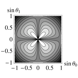
Figure 1: Contour plot of $K_{max}^{PVM}$ as a function of $\sin\theta_{0}$ and $\sin\theta_{1}$. The magnitude is represented by brightness from the maximum value of 2 (white) to the minimum value of 0 (black).

$K_{max}^{PVM}$ takes a simple form if we consider the special case of $\theta_{0}=-\theta_{1}\equiv\theta$ and $\phi_{0}=\phi_{1}=0$, i.e., the case where $|\psi_{0}\rangle=\cos\theta|0\rangle+\sin\theta|1\rangle$ and $|\psi_{1}\rangle=\cos\theta|0\rangle-\sin\theta|1\rangle$. A straightforward calculation yields

$$K=K_{max}(\theta)=2\cos^{2}\theta\ .$$ (7)

Thus, along the line $\theta_{0}=\pm\theta_{1}$, $K\equiv K_{max}$ varies as $2\cos^{2}\theta$. For $0\leq|\theta_{0}|\leq\frac{\pi}{4}$, the number of bits transferred per photon is between 1 and 2, with the maximum value of 2 obtained for $\theta_{0}=0$.

ii. Detection based on generalized measurements (Positive Operator Valued Measurements, POVMs). To close this section we remark that $K_{max}=2$ can be reached in a larger region of the parameters than the one given in Fig. 1. For this, one needs to perform a generalized measurement (Positive Operator Valued Measure, POVM), instead of the projective von Neumann measurement leading to Eq. (4). The POVM that one needs to perform is the one that corresponds to optimal unambiguous state discrimination [31]. Without going into details we just recall that the corresponding formulas for this case can be obtained if $\frac{1}{2}(1-|\langle\psi_{0}|\psi_{1}\rangle|^{2})$ in Eqs. (4) and (5) is replaced by $(1-|\langle\psi_{0}|\psi_{1}\rangle|)$. This, in turn, yields, in lieu of (6), $K_{max}^{POVM}$ as

$$K_{max}^{POVM}=2\frac{1-\mid|\cos\theta_{0}\cos\theta_{1}|-|\sin\theta_{0}\sin\theta_{1}|\mid}{\sin^{2}\theta_{0}+\sin^{2}\theta_{1}}\ .$$ (8)

In Fig. 2 we plot $K_{max}^{POVM}$ as a function of $\theta_{0}$ and $\theta_{1}$. We see that $K_{max}^{POVM}$ reaches its maximum value of 2 for a much larger range of $\theta_{0}$ and $\theta_{1}$ than in Fig. 1.

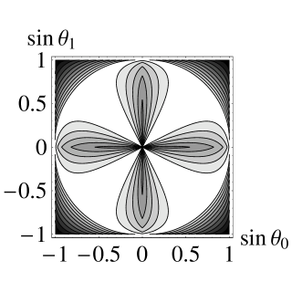
Figure 2: Contour plot of $K_{max}^{POVM}$ as a function of $\sin\theta_{0}$ and $\sin\theta_{1}$. The magnitude is represented by brightness from the maximum value of 2 (white) to the minimum value of 0 (black). A comparison to Fig. 1 reveals the advantage of a POVM: the parameter range where the maximum value of 2 can be achieved is enhanced.

A comparison of Figs. 1 and 2 reveals the advantage brought about by an optimized measurement. While the optimal POVM does not increase the value of $K_{max}$ above 2, it will increase the parameter range where the optimal value can be achieved.

For the special case of $\theta_{0}=-\theta_{1}\equiv\theta$ and $\phi_{0}=\phi_{1}=0$, considered at the end on the subsection on PVM detection, i.e., for the case where $|\psi_{0}\rangle=\cos\theta|0\rangle+\sin\theta|1\rangle$ and $|\psi_{1}\rangle=\cos\theta|0\rangle-\sin\theta|1\rangle$, $K_{max}^{POVM}=2$ along the line $-\frac{\pi}{4}\leq\theta_{0}=\pm\theta_{1}\leq\frac{\pi}{4}$. Thus, the number of bits transferred per photon is 2 for a large range of the parameters, using the optimized measurement.

4 Effect of photon losses

Photon losses can be particularly damaging to QKD schemes using VOPQs, because they induce errors caused by misidentification of the single photon state $|1\rangle$ with the vacuum $|0\rangle$. In this section we study effects of the photon losses on our generalized B92 scheme using VOPQs.

The effect of the loss of a photon is represented by amplitude damping which transforms the signal in state $|\psi_{j}\rangle=\cos\theta_{j}|0\rangle+e^{i\phi_{j}}\sin\theta_{j}|1\rangle(j=0,1)$ into a mixed state described by the density matrix

$$\rho^{\prime}_{j}=\left(\begin{array}[]{cc}\cos^{2}\theta_{j}+\gamma\sin^{2}\theta_{j}&\sqrt{1-\gamma}e^{-i\phi_{j}}\cos\theta_{j}\sin\theta_{j}\\ \sqrt{1-\gamma}e^{i\phi_{j}}\cos\theta_{j}\sin\theta_{j}&(1-\gamma)\sin^{2}\theta_{j}\end{array}\right),$$ (11)

where $\gamma$ is the probability of losing a photon. Considering only the photon losses during the fiber transmission, we express $\gamma$ as

$$\gamma=1-10^{-\alpha l/10},$$ (13)

where $\alpha$ is the loss coefficient of the fiber and $l$ the length of the fiber.

With the possibility of photon losses, Alice and Bob now face the difficulty that the signal transmission through Bob’s analyzer does not necessarily give the correct identification of the signal state. In order to ensure that our scheme works properly, we require, as a minimum condition, that the probability for correct identification be greater than the probability for incorrect identification, i.e., we require

$$\min\{Tr(\rho^{\prime}_{0}P^{\bot}_{1}),Tr(\rho^{\prime}_{1}P^{\bot}_{0})\}>\max\{Tr(\rho^{\prime}_{0}P^{\bot}_{0}),Tr(\rho^{\prime}_{1}P^{\bot}_{1})\},$$

where $\min$ and $\max$, respectively, indicate that the smaller and greater of the two are to be taken. Since the probability for incorrect identification increases with $\gamma$, the inequality (11) sets the upper limit $\gamma_{\max}$ on $\gamma$, which in turn sets the upper limit $l_{max}$ on the key transfer distance $l$.

In order to illustrate the effect of photon losses, we consider the case for which $|\psi_{0}\rangle=\cos\theta_{0}|0\rangle+\sin\theta_{0}|1\rangle$ and $|\psi_{1}\rangle=\cos\theta_{1}|0\rangle-\sin\theta_{1}|1\rangle$, and compute $\gamma_{\max}$ and $l_{\max}$ for a fixed value of $\cos^{2}\theta_{0}=0.95$ and different values of $\cos^{2}\theta_{1}$. For our calculation of $l_{\max}$, we choose $\alpha=0.2dB/km$, which is an appropriate value for fiber transmission at $1550nm$. The result of our calculation is shown in Figure 3. We see from Fig.3 that, as the value of $\cos^{2}\theta_{1}$ is moved away from $\cos^{2}\theta_{0}=0.95$ toward a smaller value, $\gamma_{max}$ and $l_{max}$ decrease and thus the amount of photon losses that can be tolerated decreases. This can be understood by noting that, as $\cos^{2}\theta_{1}$ is decreased, the signal state $|\psi_{1}\rangle$ moves toward the one-photon state and has therefore more to lose when photon losses occur. In fact, one sees from Eq.(9) that photon losses increase (decrease) the probability to find the signal in state $|0\rangle$ ($|1\rangle$) by $\gamma\sin^{2}\theta$. The smaller $\cos^{2}\theta_{1}$ is, the greater the change in the signal state due to photon losses is, and thus the greater the probability for incorrect identification of the state becomes. It is interesting to note, however, that $\gamma_{max}$ decreases sufficiently slowly with respect to $\cos^{2}\theta_{1}$ that the tolerable amount of photon losses remains high $(\gamma_{max}\gtrsim 0.8)$, as long as $\cos^{2}\theta_{1}$ is reasonably close to $\cos^{2}\theta_{0}$. On the other hand, the maximum key transfer distance decreases rapidly to less than $\sim 100km$, as $\cos^{2}\theta_{1}$ is moved away from $\cos^{2}\theta_{0}$. We note, however, that, as $\cos^{2}\theta_{1}$ is moved away from $\cos^{2}\theta_{0}$, the probability $\frac{1}{2}(1-\left|\langle\psi_{0}|\psi_{1}\rangle\right|^{2})$ for Bob to obtain a conclusive measurement outcome increases. We also remark that the photon loss probability $\gamma_{max}$ at which the probability for correct identification of the signal state is equal to the probability for incorrect identification takes on the same value regardless of whether Bob performs PVM or POVM. Hence, Fig.3 applies also to the case when POVM is performed.

Figure 3: $\gamma_{max}$(solid curve) and $l_{max}$(dotted curve) as a function of $\cos^{2}\theta_{1}$. $\cos^{2}\theta_{0}=0.95$ and $\alpha=0.2dB/km$.

Figure 4: $\gamma_{0}$ as a function of $\cos^{2}\theta_{1}$ for the case of PVM(solid curve) and POVM(dotted curve). $\cos^{2}\theta_{0}=0.95$.

The photon losses decrease the key rate and thus the parameters H and K by a factor of $(1-\gamma)$. If $\gamma$ is not too large, however, the parameter K can still be greater than $1$ with our scheme using VOPQs. In Fig.4 we plot $\gamma_{0}$ at which $K=1$ as a function of $\cos^{2}\theta_{1}$ for the same case for which Fig.3 is drawn. If $0\leq\gamma<\gamma_{0}$, then $K>1$ and thus more than one bit of classical information per photon can still be transferred in the presence of photon losses. We see again from Fig.4 the advantage brought about by POVM as compared with PVM.

5 Eavesdropping attacks

In this section we discuss effects of eavesdropping attacks on our key distribution scheme using VOPQs. For concreteness of discussion we consider the intercept-resend attack in which Eve intercepts all the signals from Alice and resends to Bob only those that give her the conclusive measurement outcome. If Alice and Bob are to detect such eavesdropping attacks, it must be required that the probability $\gamma$ of losing a photon be less than the probability $P_{?}$ that Eve’s measurement yields an inconclusive outcome, i.e., we have the requirement on $\gamma$ which reads

$$\gamma<P_{?}$$ (15)

Eq.(12) imposes another condition on $\gamma$ in addition to the condition derived from Eq.(11).

Let us take, as an example, the case $|\psi_{0}\rangle=\cos\theta|0\rangle+\sin\theta|1\rangle$ and $|\psi_{1}\rangle=\cos\theta|0\rangle-\sin\theta|1\rangle$. Assuming that Eve performs POVM on the signal from Alice, we have $P_{?}=\left|2\cos^{2}\theta-1\right|$ and thus Eq.(12) becomes $\gamma<\left|2\cos^{2}\theta-1\right|$. If $\theta$ is close to 0, that is, if $|\psi_{0}\rangle$ and $|\psi_{1}\rangle$ are both close to vacuum and thus there is a high probability for Eve to obtain the inconclusive measurement outcome, then the requirement on $\gamma$ is not so strong. As long as $\gamma$ is not too large, Alice and Bob can detect eavesdropping attacks, assuming that Eve blocks all the signals for which she obtains the inconclusive measurement outcome. On the other hand, if $\theta$ is close to $\frac{\pi}{4}$, i.e., if $|\psi_{0}\rangle$ and $|\psi_{1}\rangle$ are almost orthogonal to each other and therefore there is only a low probability for the inconclusive measurement outcome, then the requirement on $\gamma$ is strong. Alice and Bob are forced to use a low-loss system or are limited to relatively small distances for secure key distribution.

If Alice and Bob find that signal losses are higher than those expected from system losses $\gamma$, they suspect the presence of Eve and should discard all the data and restart. They keep the data only when signal losses are within the limit allowed by system losses only. The parameters H and K are therefore still limited by system losses, being reduced by a factor of $(1-\gamma)$ compared with the values in an ideal situation, even if eavesdropping attacks are considered. It should be mentioned, however, that, in our discussion so far, we have neglected the reduction of the key length caused by the acts of information reconciliation and privacy amplification that Alice and Bob need to perform to increase the accuracy and security of their shared key. The actual values of H and K will therefore be further reduced. Considering photon losses and effects of information reconciliation and privacy amplification, the cost effectiveness parameter K cannot reach its ideal maximum value of 2. It can, however, be still greater than 1, if photon losses are sufficiently small and information reconciliation and privacy amplification are efficiently performed. It is possible to securely transfer more than 1 bit of classical information per photon sent using VOPQs.

6 Discussion and Conclusion

As described in the previous sections, QKD schemes with VOPQs have the potential of transferring more than one bit of classical information per photon. When the B92 protocol is considered, the number of bits transferred per photon has an upper bound of 2. The physical reason for the existence of the upper bound on K can be understood as follows. One might naively expect that K (number of bits transferred per particle sent) can be made arbitrarily large simply by choosing the qubit states $|\psi_{0}\rangle$ and $|\psi_{1}\rangle$ arbitrarily close to vacuum, i.e., by choosing $\theta_{0}$ and $\theta_{1}$ arbitrarily close to 0, thereby reducing the number of particles sent from Alice to Bob. This expectation is, however, inaccurate because, as both $\theta_{0}$ and $\theta_{1}$ approach 0 together, the two states $|\psi_{0}\rangle$ and $|\psi_{1}\rangle$ approach each other and it becomes increasingly difficult to distinguish between them, reducing also the number of bits that can be transferred. The maximum value of 2, however, is nontrivial, because it does not correspond to the case when the average photon number per signal is 1/2.

The fact that K can be as large as 2 indicates that two bits of classical information can be securely transferred by sending just one photon, if VOPQs are employed. In practice, of course, the actual value of K should be lower than 2, because a part of the sifted key is used for checking against eavesdropping and also for information reconciliation and privacy amplification as described in Sec. 5.

It should be noted that, as $\theta_{0}$ and $\theta_{1}$ approach 0, the value of K increases, but at the same time the probability for Bob to obtain a conclusive measurement outcome decreases, which works to reduce the key rate. For example, when we consider the simple case in which $|\psi_{0}\rangle=\cos\theta|0\rangle+\sin\theta|1\rangle$ and $|\psi_{1}\rangle=\cos\theta|0\rangle-\sin\theta|1\rangle$, the key rate is given by $(r\sin^{2}2\theta)/2$, where $r$ denotes the raw key rate, i.e., the number of qubits that Alice sends to Bob in unit time. Obviously, the key rate approaches 0 as $\theta$ approaches 0. In practice, therefore, a compromise should be made between the cost effectiveness which pushes $\theta$ toward 0 and the key rate which pushes $\theta$ toward $\frac{\pi}{4}$. Clearly, $2\theta=\pi/4$ is a good compromise, in agreement with the original suggestion in the B92 protocol [24], and still comfortably achieves $K_{max}=2$ if the optimal POVM is employed for the detection of the coding states.

We mention that the efficiency of a QKD protocol has also been investigated recently by Cabello [30]. While we consider here the possibility of going beyond the Holevo limit, he studied the efficiency of QKD protocols within the Holevo limit. He considered a parameter E defined as the number of secret bits transferred per qubit per classical bit of information exchanged between Alice and Bob through a classical channel. Since the classical communication between Alice and Bob is generally necessary in a QKD protocol, we have $E\leq H$. For example, we have $E=\frac{1}{4}$ while $H=\frac{1}{2}$ for the standard BB84 protocol. Cabello has shown that it is possible to design a protocol for which Bob’s state discrimination succeeds with $100\%$ probability and thus no classical communication is needed. In such a case, the parameter E is equal to $H$ and can take on its maximum value $E=1$ in the Holevo limit.

Although QKD schemes with VOPQs have an advantage of being cost effective, they suffer from a practical difficulty of having to deal with superpositions of the vacuum and one-photon states. Another difficulty is with channel losses that are inevitably present. While channel losses reduce the key rate in the usual QKD schemes employing polarization or phase coding, they induce errors in QKD schemes with VOPQs. The requirement on channel losses for a successful execution of the QKD schemes with VOPQs is more stringent than that with other types of qubits, as shown in Sec. 4.

In conclusion, we have shown that QKD schemes with VOPQs are capable of transferring more than one bit of classical information per particle. When the B92 protocol is chosen, a maximum of two bits per photon can be securely transferred in an ideal situation with the use of vacuum-one-photon qubits. This maximal transfer rate can be reached in a large range of parameters if the optimal unambiguous discrimantion strategy is used for the detection of the coding states.

- [1] C. H. Bennett and G. Brassard: in Proceedings of the IEEE International Conference on Computers, Systems and Signal Processing, Bangalore, India (IEEE, New York, 1984), 1996.
- [2] C. H. Bennett, F. Bessette, G. Brassard, L. Salvail, and J. Smolin: J. Cryptology 5, 3 (1992).
- [3] N. Gisin, G. Riborty, W. Tittel, and H. Zbinden: Rev. Mod. Phys. 74, 145 (2002).
- [4] A. P. Lund and T.C. Ralph: Phys. Rev. A 66, 032307 (2002).
- [5] D.T. Pegg, L.S. Phillips, and S.M. Barnett: Phys. Rev. Lett. 81, 1604 (1998).
- [6] M. Dakna, J. Clausen, L. Knöll, and D.-G. Welsch: Phys. Rev. A 59, 1658 (1999).
- [7] G. M. D’Ariano, L. Maccone, M. G. A. Paris, and M. F. Sacchi: Phys. Rev. A 61, 053817 (2000).
- [8] M. G. A. Paris: Phys. Rev. A 62, 033813 (2000).
- [9] K. J. Resch, J. S. Lundeen, and A. M. Steinberg: Phys. Rev. Lett. 88, 113601 (2002).
- [10] A. I. Lvovsky and J. Mlynek: Phys. Rev. Lett. 88, 250401 (2002).
- [11] L. Davidovich, N. Zagury, M. Brune, J. M. Raimond, and S. Haroche: Phys. Rev. A 50, R895 (1994).
- [12] M. H. Y. Moussa and B. Baseia: Phys. Lett A 245, 335 (1998).
- [13] M. Freyberger: Phys. Rev. A 51, 3347 (1995).
- [14] H. W. Lee and J. Kim: Phys. Rev. A 63, 012305 (2000).
- [15] H. W. Lee: Phys. Rev. A 64, 014302 (2001).
- [16] C. J. Villas-Boas, N. G. de Almeida, and M. H. Y. Moussa: Phys. Rev. A 60, 2759 (1999).
- [17] M. Koniorczyk, Z. Kurucz, A. Gábris, and J. Janszky: Phys. Rev. A 62, 013802 (2000).
- [18] S. A. Babichev, J. Ries, and A. I. Lvovsky: Europhys. Lett. 64, 1 (2003).
- [19] E. Lombardi, F. Sciarrino, S. Popescu, and F. De Martini: Phys. Rev. Lett. 88, 070402 (2002).
- [20] S. Giacomini, F. Sciarrino, E. Lombardi, and F. De Martini: Phys. Rev. A 66, 030302(R) (2002).
- [21] S. J. van Enk: Phys. Rev. A 72, 064306 (2005).
- [22] J. W. Lee, E. K. Lee, Y.W. Chung, H. W. Lee, and J. Kim: Phys. Rev. A68, 012324 (2003).
- [23] G. L. Giorgi: Phys. Rev. A 71, 064303 (2005).
- [24] C. H. Bennett: Phys. Rev. Lett. 68, 3121 (1992).
- [25] C. E. Shannon: Bell System Tech. J. 27, 379 (1948); 27, 623 (1948).
- [26] C. M. Caves and P. D. Drummond: Rev. Mod. Phys. 66, 481 (1994)
- [27] H. P. Yuen and M. Ozawa: Phys. Rev. Lett. 70, 363 (1993)
- [28] A. S. Holevo: Probl. Inf. Transm. 9, 177 (1973).
- [29] A. S. Holevo: IEEE Trans. Inf. Theory 44, 269 (1998).
- [30] A. Cabello: Phys. Rev. Lett. 85, 5635 (2000)
- [31] For a recent review on optimized state discrimination strategies see, for example, J. A. Bergou, U. Herzog, and M. Hillery in Quantum State Estimation, edited by M. Paris and J. Řeháček: Lecture Notes in Physics, Vol. 649 (Springer, Berlin, 2004), pp. 417-465.