Stiffness dependence of critical exponents of semiflexible polymer chains situated on two-dimensional compact fractals

Abstract

We present an exact and Monte Carlo renormalization group (MCRG) study of semiflexible polymer chains on an infinite family of the plane-filling (PF) fractals. The fractals are compact, that is, their fractal dimension $d_{f}$ is equal to 2 for all members of the fractal family enumerated by the odd integer $b$ ($3\leq b<\infty$). For various values of stiffness parameter $s$ of the chain, on the PF fractals (for $3\leq b\leq 9$) we calculate exactly the critical exponents $\nu$ (associated with the mean squared end-to-end distances of polymer chain) and $\gamma$ (associated with the total number of different polymer chains). In addition, we calculate $\nu$ and $\gamma$ through the MCRG approach for $b$ up to 201. Our results show that, for each particular $b$, critical exponents are stiffness dependent functions, in such a way that the stiffer polymer chains (with smaller values of $s$) display enlarged values of $\nu$, and diminished values of $\gamma$. On the other hand, for any specific $s$, the critical exponent $\nu$ monotonically decreases, whereas the critical exponent $\gamma$ monotonically increases, with the scaling parameter $b$. We reflect on a possible relevance of the criticality of semiflexible polymer chains on the PF family of fractals to the same problem on the regular Euclidean lattices.

I Introduction

The self–avoiding walk (SAW) is a random walk that must not contain self–intersections. It has been extensively studied as a challenging problem in statistical physics, and, in particular, as a satisfactory model of a linear polymer chain vc . The pure SAW is a good model for perfectly flexible polymer, where we ignore the apparent rigidity of real polymer, and, consequently, to each step of SAW we associate the same weight factor (fugacity) $x$. In most real cases, the polymers are semiflexible with the various degree of stiffness. To take into account this property of polymers, in the continuous space models the stiffness of the SAW path is modeled by constraining the angle between the consecutive bonds of polymer, while in the lattice models, an energy barrier for each bend of the SAW is introduced. The lattice semiflexible SAW model (also known as persistent or biased SAW model), has been studied some time ago in a series of papers halley , with a focus on the so-called rod-to-coil crossover. Afterwards, it was modified in various ways, in order to describe relevant aspects of different phenomena, such as protein folding DoniachGarelOrland ; bastola , adsorption of semiflexible homopolymers kumar4 , transition between the disordered globule and the crystalline polymer phase n3 ; prellberg , behavior of semiflexible polymers in confined spaces n2 ; n4 , or influence of an external force on polymer systems kumar2 ; kumar1 ; kumar3 ; lam .

In spite of numerous studies, a scanty collection of exact results for semiflexible polymers has been achieved so far, even for the simplest lattice models. A few cases in which some properties of semiflexible SAW can be studied exactly are: directed semiflexible SAWs on regular lattices privmanKnjiga ; kumar4 , and semiflexible SAWs (with no constraints on the direction) on some fractal lattices giacometti ; tuthill . In particular, exact values of the end-to-end critical exponent $\nu$ and the entropic exponent $\gamma$ were obtained for these models, and it turned out that in some cases critical exponents are universal, whereas in other cases they depend on the stiffness of the polymer chain. Universality arguments, as well as results of approximate and extrapolation methods for similar models suggest that critical exponents on regular (Euclidean) lattices should not be affected by the value of the polymer stiffness. On the other hand, it is not known what are the effects of rigidity on the critical behavior of SAWs in nonhomogeneous environment. In order to explore further this issue, in this paper we perform the relevant study on the infinite family of the plane-filling (PF) fractal lattices d1 ; zivic3 , which allow for an exact treatment of the problem. These fractals appear to be compact, that is, their fractal dimension $d_{f}$ is equal to 2. Members of the family can be enumerated by an odd integer $b$ ($3\leq b<\infty$), and as $b\to\infty$ characteristics of these fractals approach, via the so-called fractal–to-Euclidean crossover d2 ; d3 , properties of the regular 2D lattice. By applying the exact real-space renormalization group (RG) method ex1 ; d4 , as well as Monte Carlo renormalization group (MCRG) method mc1 ; mc2 ; redner ; d6 , we calculate critical exponents $\nu$ and $\gamma$. We have performed our calculations for as many as possible members of the fractal family, for various degree of polymer stiffness, in order to study consequent stiffness dependence of the critical exponents, as well as to see the asymptotic behavior of the exponents in the fractal–to–Euclidean crossover region.

This paper is organized as follows. We define the PF family of fractals in Sec. II, where we also present the framework of our exact and MCRG approach to the evaluation of the critical exponents $\nu$ and $\gamma$ of stiff polymers on the PF fractals, together with the specific results. In Sec. III we analyze the obtained data for the critical exponents, and present an overall discussion and pertinent conclusions.

II Semiflexible polymers on the plane-filling fractal lattices

In this section we are going to apply the exact RG and the MCRG method to calculate asymptotic properties of semiflexible polymer chains on the PF fractal lattices. Each member of the PF fractal family is labelled by an odd integer $b$ ($3\leq b<\infty$), and can be constructed in stages. At the initial stage ($r=1$) the lattices are represented by the corresponding generators (see Fig. 1). The $r$th stage fractal structure can be obtained iteratively in a self-similar way, that is, by enlarging the generator by a factor $b^{r-1}$ and by replacing each of its segments with the $(r-1)$th stage structure, so that the complete fractal is obtained in the limit $r\to\infty$. The shape of the fractal generators and the way the fractals are constructed imply that each member of the family has the fractal dimension $d_{f}$ equal to 2. Thus, the PF fractals appear to be compact objects embedded in the two-dimensional Euclidean space, that is, they resemble square lattices with various degrees of inhomogeneity distributed self-similarly.

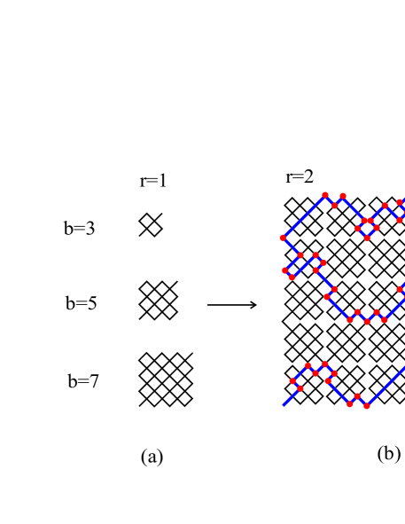
Figure 1: (Color online) (a) The first three fractal generators ($r=1$) of the plane-filling (PF) family of fractals. (b) The fractal structure of the $b=5$ PF fractal at the second stage of construction, with an example of a piece of a possible SAW path (thick line). The full dots represent the turn points of the walker (that is, the bends of the SAW path), to which we associate the Boltzmann factor $s=e^{-\Delta/k_{B}T}$, where $\Delta>0$ is the energy of SAW bend. Thus, for example, the presented SAW configuration should contribute the weight $x^{97}s^{62}$ in the corresponding RG equation (more specifically, in equation (6) for $r=0$).

In order to describe stiffness of the polymer chain, we introduce the Boltzmann factor $s={\mathrm{e}}^{-\Delta/k_{B}T}$, where $\Delta$ is an energy barrier associated with each bend of the SAW path, and $k_{B}$ is the Boltzmann constant. For $0<s<1$ $(0<\Delta<\infty)$ we deal with the semiflexible polymer chain, whereas in the limits $s=1$ $(\Delta=0)$ and $s=0$ $(\Delta=\infty)$ the polymer is a flexible chain or a rigid rod, respectively. If we assign the weight $x$ to each step of the SAW, then the weight of a walk having $N$ steps, with $N_{b}$ bends, is $x^{N}s^{N_{b}}$, and consequently, the general form of the SAW generating function can be written as

$$G(x,s)=\sum_{N=1}^{\infty}\sum_{N_{b}=0}^{N-1}C(N,N_{b})x^{N}s^{N_{b}}\>,$$ (1)

where $C(N,N_{b})$ is the number of $N$–step SAWs having $N_{b}$ bends. For large $N$, it is generally expected vc that the total number $C(N,s)=\sum_{N_{b}=0}^{N-1}C(N,N_{b})s^{N_{b}}$ of $N$–step SAW displays the following power law

$$C(N,s)\sim\mu^{N}N^{\gamma-1}\>,$$ (2)

where $\gamma$ is the entropic critical exponent, and $\mu$ is the connectivity constant. Accordingly, at the critical fugacity $x_{c}=1/\mu(s)$, we expect the following singular behavior of the above generating function

$$G_{sing}\sim{(x_{c}-x)}^{-\gamma}\>.$$ (3)

On the other hand, due to the self-similarity of the underlying structure, an arbitrary SAW configuration on the PF fractals can be described, by using the three restricted generating functions $A^{(r)}$, $B^{(r)}$ and $C^{(r)}$ (see Fig. 2), which represent partial sums of statistical weights of all feasible walks within the $r$th stage fractal structure for the three possible kinds of SAWs. One may verify that, for arbitrary $b$, the generating function $G(x,s)$ is of the form

$$G(x,s)=\sum_{r=1}^{\infty}{1\over b^{2r}} \Biggl{\{} \!\!g_{1}(B^{(r-1)},s)\left[A^{(r-1)}\right]^{2}$$ (4)

$$+ \!\!g_{2}(B^{(r-1)},s)\left[C^{(r-1)}\right]\Biggr{\}}\>,$$

where the coefficients $g_{1}(B^{(r-1)},s)$ and $g_{2}(B^{(r-1)},s)$ are polynomials in $B^{(r-1)}$ and $s$. This structure for $G(x,s)$ stems from the fact that all possible open SAW paths can be made in only two ways, using the $r$th order structures. The functions $A^{(r)}$, $B^{(r)}$ and $C^{(r)}$ appear to be parameters in the corresponding recursion (renormalization group) equations, which have the form

$$A^{(r+1)} = a(B^{(r)},s)A^{(r)}\>,$$ (5)

$$B^{(r+1)} = b(B^{(r)},s)\>,$$ (6)

$$C^{(r+1)} = c_{1}(B^{(r)},s){(A^{(r)})}^{2}+c_{2}(B^{(r)},s)C^{(r)},$$ (7)

where the coefficients $a(B^{(r)},s)$, $b(B^{(r)},s)$ and $c_{i}(B^{(r)},s)$ $(i=1,2)$, are polynomials in terms of $B^{(r)}$ and $s$, and do not depend on $r$. The established RG transformation should be supplemented with the initial conditions: $A^{(0)}=\sqrt{x}\>,$ $B^{(0)}=x$, and $C^{(0)}=0$, that are pertinent to the fractal unit segment.

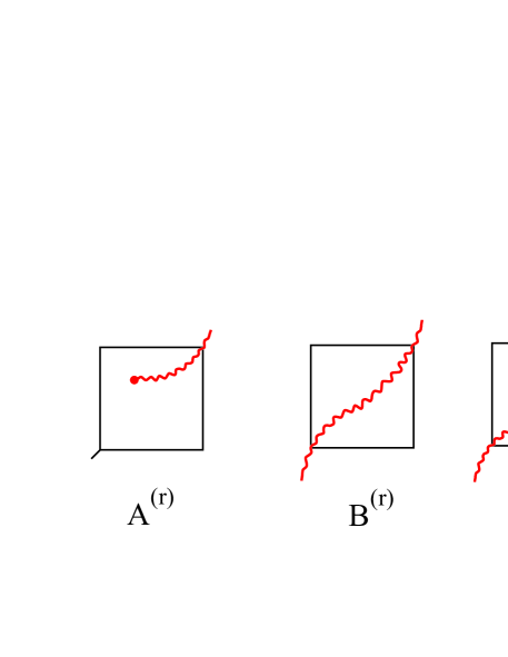
Figure 2: (Color online) A diagrammatic representation of the three restricted partition functions for an $r$th order of the fractal construction of a member of the PF family. The fractal interior structure is not shown. Thus, for example, $A^{(r)}$ represents the SAW path that starts somewhere within the fractal structure and leaves it at its upper right link to rest of fractal.

The basic asymptotic properties of SAWs are characterized by two critical exponents $\nu$ and $\gamma$. The critical exponent $\nu$ is associated with the scaling law $\left<R_{N}^{2}\right>\sim N^{2\nu}$ for the mean squared end-to-end distance for $N$-step SAW, while the critical exponent $\gamma$ is associated with the total number of distinct SAWs described by (2), for very large $N$ vc . We start by applying the above RG approach to find the critical exponent $\nu$ for semiflexible polymers on PF fractals. We shall first present the corresponding exact calculation, and then we shall expound on the MCRG approach. To this end, we need to analyze (6) at the corresponding fixed point. It can be shown that $b(B^{(r)},s)$ in (6) is a polynomial

$$B^{\prime}=\sum_{N,N_{b}}P(N,N_{b})B^{N}s^{N_{b}}\>,$$ (8)

where we have used the prime for the $r$th order partition function and no indices for the $(r-1)$th order partition function. Knowing the RG equation (8), value of the critical exponent $\nu$ follows from the formula d4

$$\nu={\ln b\over\ln\lambda_{\nu}}\>,$$ (9)

where $\lambda_{\nu}$ is the relevant eigenvalue of the RG equation (8) at the nontrivial fixed point $0<B^{*}(s)<1$, that is

$$\lambda_{\nu}={dB^{\prime}\over dB}\biggm{|}_{B^{*}}\>.$$ (10)

Consequently, evaluation of $\nu$ starts with determining the coefficients $P(N,N_{b})$ of (8) and finding the pertinent fixed point value $B^{*}(s)$, which is, according to the initial condition $B^{(0)}=x$, equal to the critical fugacity $x_{c}=1/\mu$.

We have been able to find exact values of $P(N,N_{b})$ for $3\leq b\leq 9$. For the first two fractals ($b=3$ and 5) the RG equation (8) has the form

$$B^{\prime} = B^{3}+2B^{5}s^{4}\>,$$ (11)

$$B^{\prime} = B^{5}+12B^{7}s^{4}+2B^{9}s^{4}+12B^{9}s^{6}+6B^{9}s^{8}+$$

$$4B^{11}s^{6}+8B^{11}s^{8}+2B^{13}s^{8}+4B^{13}s^{10}+2B^{15}s^{12},$$

respectively, while for $b=7$ and 9 they are disposed within the Electronic Physics Auxiliary Publication Service (EPAPS) supp . Knowing $P(N,N_{b})$, for a given $b$, we use Eqs. (8)–(10) to learn $B^{*}(s)$ and the critical exponent $\nu(s)$. For the $b=3$ PF fractal the critical fugacity $B^{*}$ and the critical exponent $\nu$ can be obtained in the closed forms as functions of the stiffness parameter

$$B^{*}_{b=3}(s) = {\sqrt{\sqrt{1+8s^{4}}-1}\over 2s^{2}}\>,$$ (13)

$$\nu_{b=3}(s) = {\ln 3\over\ln\left(5-{\sqrt{1+8s^{4}}-1\over 2s^{4}}\right)}\>,$$ (14)

while for $b=5$, 7 and 9 they can only be calculated numerically. We have chosen the set of six values for the polymer stiffness parameter ($s=1,0.9,0.7,0.5,0.3$ and $s=0.1$) and the obtained exact values are presented in the Tables 1 and 2 (together with the results obtained by the MCRG method).

Table 1: The exact ($3\leq b\leq 9$) and MCRG ($11\leq b\leq 201$) results for the critical fugacities $B^{*}$ of the PF family of fractals. Each MCRG entry of the Table has been obtained by performing at least $10^{5}$ MC simulations. The numbers in the brackets represent the MCRG errors concerning the last two digits, for instance, for $b=101$ fractal the reading should be the following: $B^{*}(s=1)=0.38815(05)\equiv 0.38815\pm 0.00005$. The values for $b=\infty$ are obtained by linear extrapolation of MCRG values.

$b$	$B^{*}(s=1)$	$B^{*}(s=0.9)$	$B^{*}(s=0.7)$	$B^{*}(s=0.5)$	$B^{*}(s=0.3)$	$B^{*}(s=0.1)$
3	0.70711	0.75595	0.85923	0.94815	0.99212	0.99990
5	0.59051	0.63304	0.73677	0.86443	0.97258	0.99965
7	0.53352	0.57132	0.66544	0.79312	0.94262	0.99924
9	0.50029	0.53516	0.62208	0.74257	0.90676	0.99866
11	0.47863(23)	0.51141(24)	0.59352(26)	0.70754(27)	0.87251(13)	0.99785(05)
13	0.46319(14)	0.49449(20)	0.57335(22)	0.68289(24)	0.84351(25)	0.99679(07)
15	0.45191(13)	0.48212(18)	0.55857(20)	0.66399(21)	0.82073(22)	0.99525(08)
17	0.44321(11)	0.47307(17)	0.54733(18)	0.64984(19)	0.80218(20)	0.99315(09)
21	0.43065(10)	0.45927(06)	0.53091(07)	0.62963(16)	0.77512(17)	0.98700(10)
25	0.42207(08)	0.45005(12)	0.51956(06)	0.61549(14)	0.75663(14)	0.97767(11)
31	0.41323(06)	0.44057(10)	0.50811(11)	0.60115(15)	0.73802(12)	0.96076(10)
35	0.40913(06)	0.43611(09)	0.50276(10)	0.59441(11)	0.72923(11)	0.95010(10)
41	0.40420(04)	0.43086(06)	0.49664(04)	0.58698(10)	0.71913(10)	0.93637(08)
51	0.39893(07)	0.42498(07)	0.48969(03)	0.57825(15)	0.70797(09)	0.91977(07)
61	0.39524(06)	0.42112(06)	0.48493(07)	0.57259(07)	0.70032(08)	0.90832(08)
81	0.39081(05)	0.41638(05)	0.47933(03)	0.56545(07)	0.69079(11)	0.89413(05)
101	0.38815(05)	0.41344(06)	0.47601(11)	0.56137(06)	0.68541(06)	0.88578(08)
121	0.38649(04)	0.41167(07)	0.47373(09)	0.55862(05)	0.68184(05)	0.88007(04)
151	0.38479(02)	0.40989(09)	0.47163(04)	0.55592(08)	0.67825(05)	0.87459(11)
171	0.38399(03)	0.40894(06)	0.47054(06)	0.55464(04)	0.67668(04)	0.87217(07)
201	0.38316(06)	0.40803(02)	0.46951(11)	0.55321(09)	0.67480(04)	0.86939(09)
⋮
$\infty$	0.37915(40)	0.40189(12)	0.46217(15)	0.54424(15)	0.66287(22)	0.85186(20)

Table 2: The exact ($3\leq b\leq 9$) and MCRG ($11\leq b\leq 201$) results for the critical exponents $\nu$ obtained in this work, for the PF family of fractals. Each MCRG entry of the Table has been obtained by performing at least $10^{5}$ MC simulations. Numbers in the brackets correspond to the errors of the last two digits, determined by the MC simulation statistics (for example, for $b=11$ and $s=0.9$, we have $\nu=0.77239(27)\equiv 0.77239\pm 0.00027$).

$b$	$\nu(s=1)$	$\nu(s=0.9)$	$\nu(s=0.7)$	$\nu(s=0.5)$	$\nu(s=0.3)$	$\nu(s=0.1)$
3	0.79248	0.81384	0.87230	0.94400	0.99061	0.99988
5	0.78996	0.79864	0.82629	0.88266	0.96922	0.99959
7	0.78111	0.78666	0.80342	0.83910	0.93233	0.99906
9	0.77464	0.77886	0.79108	0.81500	0.88946	0.99813
11	0.76959(27)	0.77239(27)	0.78194(26)	0.80127(27)	0.85478(15)	0.99659(03)
13	0.76494(18)	0.76923(25)	0.77739(25)	0.79250(25)	0.83325(29)	0.99415(11)
15	0.76232(17)	0.76571(24)	0.77307(24)	0.78678(24)	0.81825(26)	0.99022(14)
17	0.75976(17)	0.76226(23)	0.76962(23)	0.78205(22)	0.80885(24)	0.98385(18)
21	0.75522(16)	0.75754(10)	0.76411(09)	0.77496(21)	0.79717(21)	0.96152(27)
25	0.75199(15)	0.75406(07)	0.76001(09)	0.77000(19)	0.78993(20)	0.92615(31)
31	0.74822(12)	0.74954(20)	0.75559(19)	0.76515(18)	0.78315(18)	0.87448(29)
35	0.74530(14)	0.74773(19)	0.75278(18)	0.76276(17)	0.77889(17)	0.85207(25)
41	0.74332(08)	0.74487(06)	0.74966(08)	0.75837(16)	0.77439(16)	0.83262(21)
51	0.73969(17)	0.74148(17)	0.74614(07)	0.75381(15)	0.76970(15)	0.81726(17)
61	0.73643(17)	0.73930(16)	0.74352(05)	0.75051(14)	0.76579(14)	0.80992(15)
81	0.73314(15)	0.73527(14)	0.73935(06)	0.74640(19)	0.76050(12)	0.80041(13)
101	0.73103(11)	0.73280(04)	0.73610(14)	0.74313(12)	0.75689(12)	0.79482(12)
121	0.72865(13)	0.73030(22)	0.73459(28)	0.74071(11)	0.75405(11)	0.79097(11)
151	0.72771(07)	0.72840(06)	0.73219(11)	0.73848(10)	0.75102(10)	0.78618(08)
171	0.72631(12)	0.72752(05)	0.73094(10)	0.73830(10)	0.74850(09)	0.78338(10)
201	0.72486(12)	0.72633(05)	0.72958(12)	0.73583(04)	0.74755(09)	0.78077(10)

To overcome the computational problem of learning exact values of $P(N,N_{b})$, for fractals with $b\geq 11$, we apply the Monte Carlo renormalization group method (MCRG) d6 . The essence of the MCRG method consists of treating $B^{\prime}$, given by (8), as the grand canonical partition function that accounts for all possible SAWs that traverse the fractal generator at two fixed apexes. In this spirit, (8) allows us to write the following relation

$${dB^{\prime}\over dB}={B^{\prime}\over B}\left<N(B)\right>\>,$$ (15)

where $\left<N(B)\right>$ is given by

$$\left<N(B,s)\right>={1\over B^{\prime}}\sum_{N,N_{b}}NP(N,N_{b})B^{N}s^{N_{b}}\>,$$ (16)

which can be considered as the average number of steps, made with fugacity $B$ and stiffness $s$, by all possible SAWs that cross the fractal generator. Then, from (8) and (10), it follows

$$\lambda_{\nu}=\left<N(B^{*},s)\right>.$$ (17)

The last formula enables us to calculate $\nu$ via the MCRG method, that is, without calculating explicitly the coefficients $P(N,N_{b})$. For a given fractal (with the scaling factor $b$) and the SAW stiffness $s$, we begin with determining the critical fugacity $B^{*}$. To this end, we start the Monte Carlo (MC) simulation with an initial guess for the fugacity $B_{0}$ in the region $0<B_{0}<1$. Here $B_{0}$ can be interpreted as the probability of making the next step along the same direction from the vertex that the walker has reached, while $sB_{0}$ is the probability to make the next step by changing the step direction. We assume that the walker starts his path at one terminus (vertex) and tries to reach the other terminus of the generator. In a case that the walker does not succeed to pass through the generator, the corresponding path is not taken into account. We repeat this MC simulation $L$ times, for the same set $B_{0}$ and $s$. Thus, we find how many times the walker has passed through the generator, and by dividing the corresponding number by $L$ we get the value of the function (8), denoted here by $B^{\prime}(B_{0},s)$. In this way we get the value of the sum (8) without specifying the set $P(N,N_{b})$. Then, for a fixed $s$, the next values $B_{n}$ $(n\geq 1)$, at which the MC simulation should be performed, can be found by using the “homing” procedure redner , which can be closed at the stage when the difference $B_{n}-B_{n-1}$ becomes less than the statistical uncertainty associated with $B_{n-1}$. Consequently, $B^{*}$ can be identified with the last value $B_{n}$ found in this way. Performing the MC simulation at the values $B^{*}$ and $s$, we can record all possible SAWs that traverse the fractal generator. Then, knowing such a set of walks, we can represent the average value of the length of a walk (that traverse the generator) via the corresponding average number of steps $\langle N(B^{*},s)\rangle$, and, accordingly, we can learn the value of the $\nu$ through the formulas (17) and (9). In Tables 1 and 2, we present our MCRG results for $B^{*}$ and $\nu$ respectively, for the chosen set of $s$ values, for the PF fractal lattices with $11\leq b\leq 201$.

To calculate the critical exponent $\gamma$ we need to find the singular behavior of the generating function $G(x,s)$. The structure of the expression (4) shows that the asymptotic behavior of $G(x,s)$, in the vicinity of the critical fugacity $x_{c}(s)$, depends on the corresponding behavior of the restricted partition functions (5)–(7). Assuming that the singular behavior of (4) is of the form (3), it can be shown zivic3 that the critical exponent $\gamma$ should be given by

$$\gamma=2{\ln(\lambda_{\gamma}/b)\over\ln\lambda_{\nu}}\>,$$ (18)

where $\lambda_{\gamma}$ is the RG eigenvalue

$$\lambda_{\gamma}=a(B^{*},s)\>,$$ (19)

of the polynomial $a(B^{(n-1)},s)$ defined by (5), with $B^{*}$ being the fixed point value of (8). Therefore, it remains either to determine exactly an explicit expression for the polynomial $a\left(B^{(n-1)},s\right)$, or somehow to surpass this step and to evaluate only the single needed value $a(B^{*},s)$. We have been able to determine the exact form of the requisite polynomial for the PF fractals with $3\leq b\leq 9$, while for $b\geq 11$ we have applied the MCRG to evaluate $a(B^{*},s)$.

Table 3: The exact ($3\leq b\leq 9$) and MCRG ($11\leq b\leq 201$) results for the critical exponents $\gamma$ obtained in this work, for the PF family of fractals. Each MCRG entry of the Table has been obtained by performing at least $5\cdot 10^{5}$ MC simulations. The numbers in the brackets represent the error bars related to the last two digits, for example for $b=201$ and $s=0.9$, we have $\gamma=2.216(13)\equiv 2.216\pm 0.013$.

$b$	$\gamma(s=1)$	$\gamma(s=0.9)$	$\gamma(s=0.7)$	$\gamma(s=0.5)$	$\gamma(s=0.3)$	$\gamma(s=0.1)$
3	1.6840	1.6796	1.6056	1.3368	0.8189	0.2524
5	1.7423	1.7406	1.7236	1.6250	1.1654	0.3363
7	1.7614	1.7605	1.7552	1.7247	1.4586	0.4302
9	1.7807	1.7795	1.7748	1.7596	1.6335	0.5340
11	1.8048(32)	1.7987(31)	1.7908(28)	1.7753(25)	1.7194(17)	0.6498(07)
13	1.8158(32)	1.8136(33)	1.8095(30)	1.8020(26)	1.7573(21)	0.7746(08)
15	1.8395(25)	1.8251(35)	1.8267(32)	1.8138(28)	1.7827(22)	0.9082(09)
17	1.8595(27)	1.8590(36)	1.8484(33)	1.8281(29)	1.7981(23)	1.0491(11)
21	1.8944(29)	1.8834(37)	1.8848(33)	1.8760(31)	1.8222(25)	1.3261(13)
25	1.9244(42)	1.9106(40)	1.9101(36)	1.8932(34)	1.8452(26)	1.5333(16)
31	1.9549(34)	1.9538(47)	1.9291(43)	1.9281(37)	1.8839(29)	1.6914(17)
35	1.9810(50)	1.9826(50)	1.9526(69)	1.9398(35)	1.9033(30)	1.7425(17)
41	1.9842(53)	1.9921(52)	1.9846(46)	1.9763(43)	1.9305(30)	1.7778(18)
51	2.0398(62)	2.0366(61)	2.0325(53)	1.9991(48)	1.9779(27)	1.8202(19)
61	2.0744(67)	2.0420(67)	2.0428(55)	2.0323(52)	1.9899(40)	1.8418(21)
81	2.0912(60)	2.0903(81)	2.0773(49)	2.0819(78)	2.0124(48)	1.8961(24)
101	2.124(17)	2.1316(95)	2.1196(77)	2.1233(73)	2.0655(54)	1.9328(27)
121	2.172(11)	2.158(12)	2.145(11)	2.1429(78)	2.1040(60)	1.9577(30)
151	2.175(13)	2.182(13)	2.182(10)	2.174(10)	2.1356(65)	1.9782(34)
171	2.191(14)	2.198(15)	2.192(13)	2.1846(94)	2.1484(79)	2.0219(35)
201	2.2154(89)	2.216(13)	2.2023(85)	2.219(14)	2.1598(86)	2.0810(42)

In order to learn an explicit expression of the polynomial $a(B^{(r-1)},s)$, we note that its form, due to the underlying self-similarity, should not depend on $r$, and, for this reason, in what follows we assume $r=1$. Then, one can verify the following expression

$$a(B,s)=\sum_{N,N_{b}}Q(N,N_{b})B^{N}s^{N_{b}}\>,$$ (20)

where $Q(N,N_{b})$ is the number of all SAWs of $N$ steps, with $N_{b}$ bends, that start at any bond within the generator ($r=1$) and leave it at a fixed exit. By enumeration of all relevant walks, the coefficients $Q(N,N_{b})$ can be evaluated exactly up to $b=9$. For $b=3$ fractal, the polynomial (20) is of the form

$$a(B,s) = 1+B+2Bs+B^{2}+2B^{2}s+2B^{2}s^{2}+2B^{3}s^{2}$$

$$+ 2B^{3}s^{3}+4B^{4}s^{3}+4B^{4}s^{4}+2B^{5}s^{4}+2B^{6}s^{5}\>,$$

for $b=5$ it is given in the Appendix, while for $b=7$ and 9 they are given in the supplementary EPAPS Document supp . Using this information, together with (19), (18), and previously found $B^{*}$ and $\lambda_{\nu}$, we have obtained the desired exact values of $\gamma$ (see Table 3).

For a sequence of $b>9$, the exact determination of the polynomial (20), that is, knowledge of the coefficients $Q(N,N_{b})$, can be hardly reached using the present-day computers. However, to calculate $\lambda_{\gamma}$ one does not need a complete knowledge of polynomial $a(B,s)$, but only its values at the fixed point (see Eq. (19)). However, the polynomial that appears in (5) can be conceived as grand partition function of an appropriate ensemble, and consequently, within the MCRG method, the requisite value of the polynomial can be determined directly zivic3 . Owing to the fact that we can obtain $\lambda_{\gamma}=a(B^{*},s)$ through the MC simulations, and, knowing $\lambda_{\nu}$ from the preceding calculation of $\nu$, we can apply (18) to calculate $\gamma$. In Table 3 we present our MCRG results of $\gamma$ for $11\leq b\leq 201$, for the chosen set of stiffness parameter values ($s=1$, 0.9, 0.7, 0.5, 0.3 and 0.1).

III Discussion and summary

We have studied critical properties of semiflexible polymer chains on the infinite family of the PF fractals whose each member has the fractal dimension $d_{f}$ equal to the Euclidean value 2. In particular, we have calculated the critical exponents $\nu$ and $\gamma$ via an exact RG (for $3\leq b\leq 9$) and via the MCRG approach (up to $b=201$). Specific results for the critical exponents have been presented in Tables 2 and 3.

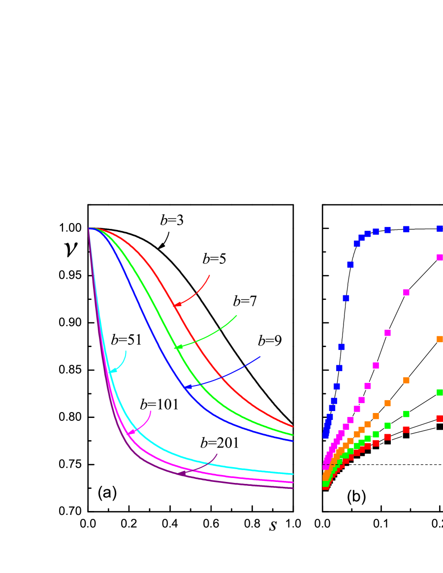
Figure 3: (Color online) Plot of the end-to-end distance critical exponent $\nu$ of semiflexible polymer chain on PF fractals: (a) as a function of stiffness parameter $s$, for various fractal scaling parameter $b$, and (b) as a function of $1/b$, for various values of stiffness parameter $s$ (the horizontal dashed line represents the Euclidean value $\nu=3/4$ for flexible polymers, $s=1$, whereas thin solid lines serve only as guides to the eye).

In order to analyze the obtained results, in Fig. 3(a) we have plotted $\nu$ as a function of stiffness parameter $s$, for several values of fractal scaling parameter $b$. One can see that for each $b$, exponent $\nu$ monotonically decreases from the value $\nu=1$, for $s=0$, corresponding to rigid rod, to the value $\nu_{SAW}(b)$, for $s=1$, corresponding to the flexible polymer chain z12 ; zivic3 . This, indeed, implies that for finite $b$, the mean end-to-end distance for semiflexible polymers increases with its rigidity, and is always between its values for the flexible chain and the rigid rod. In the same figure one can also observe that when $b$ increases the curves $\nu(s)$ become increasingly sharper so that their limit looks to be $\nu=1$, at $s=0$, whereas $\nu\approx\text{const.}$, for $0<s\leq 1$. This observation may imply that for very large $b$ (beyond $b=201$) the critical exponent $\nu$ becomes independent of $s$. Here, one should note that it is believed that critical exponent $\nu$ is universal for semiflexible SAWs on Euclidean lattices, that is, it does not depend on $s$ giacometti . This expectation is based on universality arguments, and it was exactly demonstrated for directed semiflexible SAWs privmanKnjiga . The same conclusion was also exactly derived for semiflexible SAWs on the Havlin–Ben-Avraham and 3-simplex fractal lattices giacometti . However, as it was pointed out in giacometti , in contrast to the case of homogeneous lattices, where rigidity only increases the persistence length, but does not affect neither the scaling law governing the critical behavior of the the mean end-to-end distance, nor the value of the critical exponent $\nu$ of SAWs, one might expect that presence of disorder in nonhomogeneous lattices, combined with the stiffness, in some cases can constrain the persistence length, and consequently induces dependence of $\nu$ on $s$. This was explicitly confirmed in the same paper, by exact calculation of the critical exponent $\nu$ for branching Koch curve, which turned out to be continuously decreasing function of $s$, similar to functions depicted in Fig. 3(a). Apparently, the established dependence of $\nu$ on $s$ for PF fractals with smaller values of $b$ shows that considerable lattice disorder affects significantly the values of $\nu$, while the dependence of $\nu$ on $s$ gradually disappears for PF fractals with smaller disorder (appearing for larger $b$). These facts confirm the assumption giacometti that lattice disorder, combined with the polymer stiffness, has a predominant impact on the critical behavior of semiflexible polymers.

In Fig. 3(b) data for $\nu$ as a function of $1/b$ are depicted, for various values of $s$. It appears that for each considered value of stiffness $s$ in the range $0<s\leq 1$, the critical exponent $\nu$ is monotonic function of the scaling parameter $b$, in the region of $b$ studied. It can be also seen that for large fixed $b$, the differences between the values of $\nu(s)$ (for various $s$) decrease when $b$ increases, which brings us to the question of the behavior of $\nu$ in the fractal–to–Euclidean crossover, when $b\to\infty$. Concept of the fractal-to-Euclidean crossover is often used in order to study if and how various physical properties change when inhomogeneous lattices approach homogeneous (translationally invariant Euclidean) lattice. By tuning some conveniently chosen parameter of the fractal lattice (such as scaling parameter $b$ in the case of PF fractals), properties of the corresponding Euclidean lattice (square lattice in this case) can be gradually approached. Studies of the flexible SAW models on Sierpinski gasket family of fractals d3 ; d6 ; p1 ; p2 ; p3 ; d7 ; d8 , as well as on PF fractals zivic3 , revealed that crossover behavior of critical exponents can be rather subtle in the sense that not all critical exponents tend to their Euclidean values, and even when they do so it can be accomplished in quite unexpected manner. For instance, according to the finite–size scaling arguments, when $b\to\infty$ exponent $\nu$ of flexible polymers ($s=1$) on PF fractals approaches the Euclidean value 3/4 from below zivic3 , which together with the fact that $\nu$ is monotonically decreasing function for $b$ up to $201$, means that for some value of $b$ larger than 201 there should exist a minimum. On the other hand, for $s=0$ exponent $\nu$ is equal to 1 for each $b$. For $0<s\leq 1$ apparent trend of the curves presented in Fig. 3(b) suggests that limiting value of $\nu$, when $b\to\infty$, does not depend on particular value of $s$, and following the behavior of $\nu$ for flexible polymers, it should be equal to the Euclidean value $3/4$. However, we would not like to draw here such a definite conclusion without additional investigations.

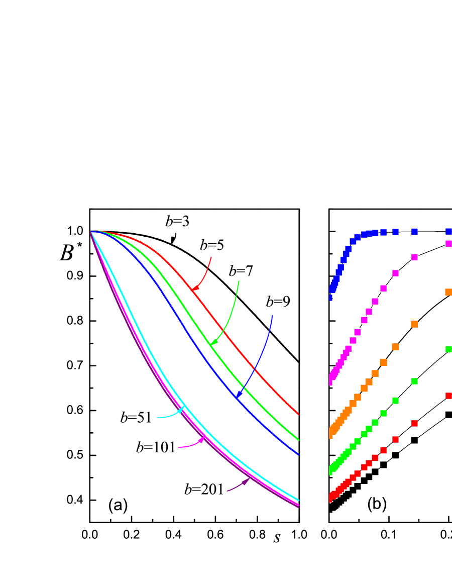
Figure 4: (Color online) Data for the fixed point values $B^{*}$ (the reciprocal connectivity) of semiflexible polymer chain plotted as: (a) function of stiffness $s$, for various values of the fractal parameter $b$, and (b) function of $1/b$, for various values of $s$.

Continuing the comparison of the criticality of flexible and semiflexible SAWs on the PF fractals, in Fig. 4 we have depicted the data from Table 1 for the critical fixed points $B^{*}$. On the left-hand side of this figure one can notice that $B^{*}$, which is equal to the reciprocal of the connectivity constant $\mu$, is monotonically decreasing function of $s$, for each $b$ considered. This has been expected, since $\mu$ has the physical meaning of the average number of steps available to the walker having already completed a large number of steps, so that larger flexibility of the polymer chain implies larger $\mu$, and consequently $\mu(s=0)<\mu(0<s<1)<\mu(s=1)$. In Fig. 4(b) one can also observe that for fixed $s$, the fixed point $B^{*}$ decreases with $b$. Furthermore, $B^{*}$ becomes almost linear function of $1/b$ for large $b$, which allows us to estimate the limiting values of $B^{*}$ for $b\to\infty$. The obtained asymptotic values are given at the end of Table 1. The value $B^{*}(s=1)=0.37915\pm 0.00040$, should be compared with the Euclidean value 0.3790523(3) for the square lattice, obtained in guttmann . As one can see, the agreement is very good, and we may say that for flexible polymers the values $B^{*}(b)$, in the limit $b\to\infty$, converge to the Euclidean value. Similarly, we expect that, for given $s<1$, the values $B^{*}(b)$ of semiflexible polymers also converge to the corresponding $d=2$ Euclidean values (which are functions of $s$). In Fig. 5(a) we have plotted the lines obtained by linear fitting of the large $b$ data for $B^{*}(s)$ for $s=0.1$, 0.3, 0.5, 0.7, 0.9 and $s=1$. In the present situation, estimated limiting values of the connectivity constants $\mu(s)=1/B^{*}(s,b\to\infty)$ are depicted in Fig. 5(b), as function of $s$. It seems that $\mu(s)$ is linear function of $s$, implying that connectivity constant for semiflexible SAWs on square lattice could be a linear function of the stiffness parameter $s$. Such expectation is also in accord with the exact results obtained for directed semiflexible SAWs privmanKnjiga .

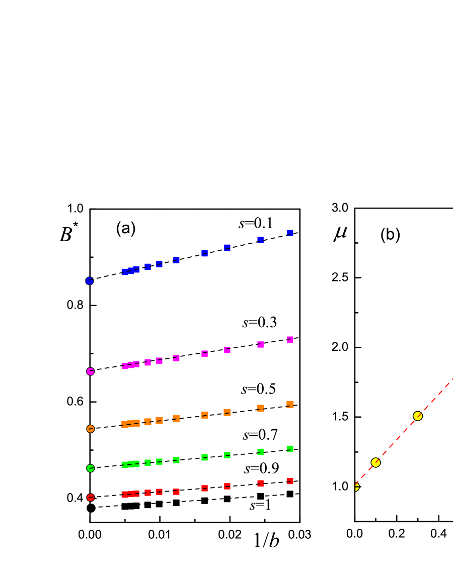
Figure 5: (Color online) (a) Linear fitting of the data (full squares) for the fixed point $B^{*}$ (see Table 1) as function of $1/b$ for large values of $b$, and various $s$. Circles correspond to the extrapolated limiting values of $B^{*}(s,b\to\infty)$, and their precise values are given in the last row of Table 1. (b) Plot of the connectivity constant $\mu(s)=1/B^{*}(s,b\to\infty)$. Dashed line is the linear fit of the data presented by circles, which correspond to $\mu(s)$ for $s=0$, 0.1, 0.3, 0.5, 0.7, 0.9 and $s=1$.

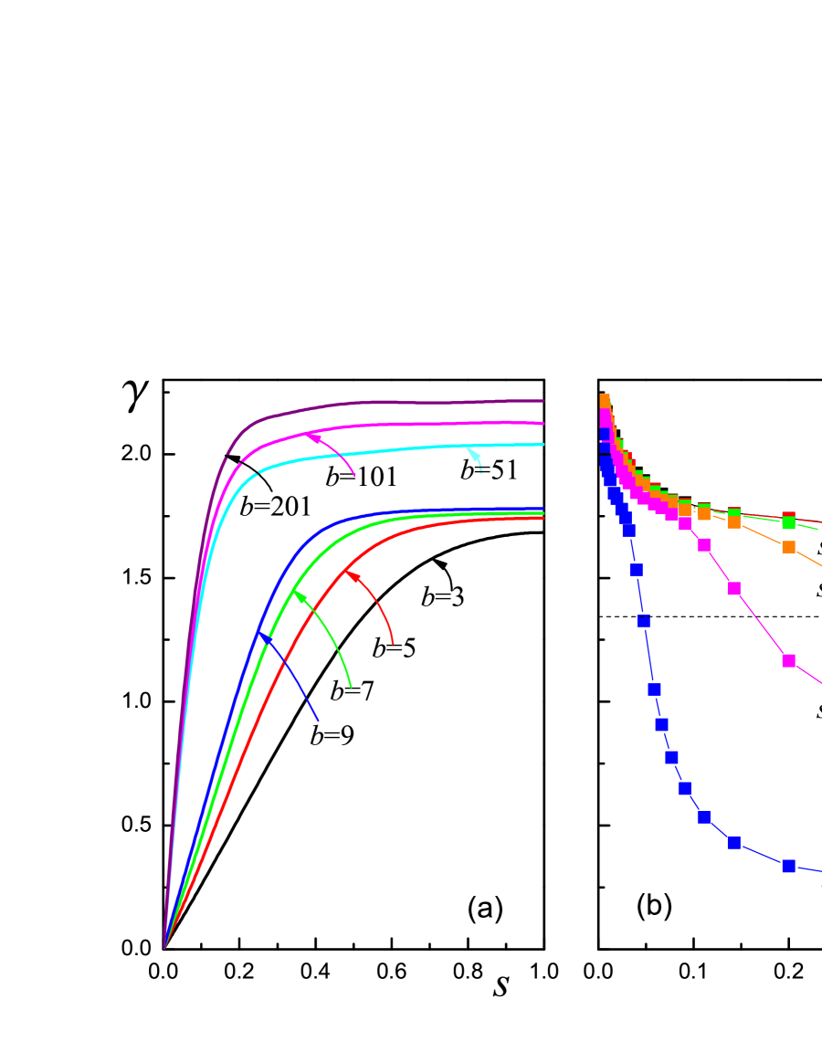
Figure 6: (Color online) Data for the SAW critical exponent $\gamma$ presented as: (a) function of the stiffness parameter $s$, for various values of the fractal enumerator $b$, and (b) function of $1/b$, for $s=1$, 0.9, 0.7, 0.5, 0.3, and 0.1 (the horizontal dashed line represents the two–dimensional Euclidean value $\gamma=43/32$ for flexible polymers $s=1$).

To make our analysis of semiflexible SAWs on PF fractals complete, in Fig. 6 we present the data found for the critical exponent $\gamma$. As it was explained in Sec. II, exponent $\gamma$ is given by (18): $\gamma=2\ln(\lambda_{\gamma}/b)/\ln\lambda_{\nu}$, where eigenvalues $\lambda_{\nu}$ and $\lambda_{\gamma}$ (given by (10) and (19), respectively) are evaluated at the fixed point $B=B^{*}$ of the RG equation (6). For $b=3$ the fixed point $B^{*}$ is given by (13), and since dependence of $\lambda_{\nu}$ and $\lambda_{\gamma}$ on $B$ is known by exact means, the curve $\gamma(b=3,s)$ in Fig. 6(a) was plotted according to the closed-form exact formula. For $b=5$, 7 and 9, RG equation (6) was also found explicitly, but its fixed point can be calculated only numerically in these cases. Nevertheless, this task can be done for large number of $s$ values, and putting fixed points $B^{*}(s)$ calculated accordingly, into the exact expressions found for $\lambda_{\nu}$ and $\lambda_{\gamma}$, one obtains the corresponding values for $\gamma$, and, consequently, curves for $b=5$, 7 and 9 in Fig. 6(a). For larger values of $b$, depicted $\gamma$ curves were obtained by interpolating the data found by MCRG approach for $s=0.1$, 0.3, 0.5, 0.7, 0.9 and $s=1$ (Table 3), and generalizing the fact $\gamma(b,s=0)=0$, exactly found for smaller values of $b$, to all $b$ values. One can see that for each $b$, the critical exponent $\gamma$ is monotonically increasing function of the stiffness parameter $s$. The dependence of $\gamma$ on $s$ is in accord with the discussed non-universality of $\nu$, and also with the results obtained for $\gamma$ of SAWs on the branching Koch curve and Havlin–Ben-Avraham fractal giacometti . However, one should note here that while for the Koch curve both $\nu$ and $\gamma$ depend on $s$, in the case of Havlin–Ben-Avraham fractal only $\gamma$ is non-universal ($\nu=1$ for all values of $s$). Besides, in giacometti it was shown that neither $\nu$ nor $\gamma$ depend on $s$ for SAWs on the 3-simplex fractal. The observed different behavior of exponents $\nu$ and $\gamma$ on various fractals is an intriguing fact and imposes the question of the universality of $\gamma$ for semiflexible SAWs on homogeneous lattices. One might try to draw a helpful conclusion by looking at the large $b$ behavior of the functions $\gamma(s)$, plotted in Fig. 6(a). One can see that as $b$ grows the curve $\gamma(s)$ becomes sharper, so that for $b=201$ it is almost constant in the large part of the region $0<s\leq 1$, whereas in the vicinity of $s=0$ it rapidly drops to the value $\gamma=0$, at $s=0$. Therefore, it may be concluded that for $b\gg 1$ and $0<s\leq 1$ exponent $\gamma$ becomes independent of $s$. Furthermore, in Fig. 6(b), we perceive that for each studied $s$, the critical exponents $\gamma$ monotonically increase with $b$, and for $b=201$ acquire almost the same value $\gamma\approx 2.2$. These observations may imply that $\gamma$ for semiflexible SAWs on homogeneous lattices is universal. However, it is known that critical exponent $\gamma$ for flexible polymers ($s=1$) on the two-dimensional Euclidean lattices is equal to $\gamma=43/32$, which is far from the apparent limiting value 2.2 (suggested by the plots in Fig. 6(b), when $1/b\to 0$), implying that $\gamma$ for PF fractals does not tend to its Euclidean value for large $b$. This may seem odd, but it fits quite well into the peculiar picture which have emerged during the last two decades for the fractal-to-Euclidean crossover behavior of the exponent $\gamma$ of flexible SAWs on PF zivic3 and on Sierpinski gasket (SG) family of fractals d3 ; d7 ; d8 , as well as for some models of directed SAWs on SG fractals p3 . For instance, using finite-size scaling arguments, Dhar d3 concluded that $\gamma$ for SAWs on SG fractals at the fractal-to-Euclidean crossover approaches the non-Euclidean value 133/32. In a similar manner, for PF fractals it was also demonstrated zivic3 that in the limit $b\to\infty$ exponent $\gamma$ tends to $103/32$, which is again the non-Euclidean value. In addition, numerical analysis of the large set of exact values of $\gamma$ obtained for the piece-wise directed SAWs on SG fractals, as well as an exact asymptotic analysis p3 , also showed that the limiting value of $\gamma$ differs from the corresponding Euclidean value. In all these cases the established crossover behavior could not have been predicted only on the basis of $\gamma$ values obtained for relatively small $b$ (up to $b=201$, for instance). On these grounds we may infer that in the crossover region, when $b\to\infty$, critical exponent $\gamma$ does not depend on the stiffness $s$, and approaches the non-Euclidean value.

In conclusion, we may say that family of plane-filling fractals proved to be useful for investigation of the effects of the rigidity on the criticality of SAWs on nonhomogeneous lattices. It is amenable to applying exact and Monte Carlo renormalization group study, which we performed on large number of its members. The obtained results show that the critical behavior of semiflexible SAWs is not universal, in a sense that critical end-to-end exponents $\nu$, as well as entropic exponents $\gamma$, continuously vary with the stiffness parameter $s$. Such non-universality does not occur on regular lattices, but it was found for SAWs on the branching Koch curve, suggesting that polymer behavior in realistic disordered environment might be more affected by its stiffness than it was expected. Apart from the stiffness parameter $s$, critical exponents also depend on the fractal parameter $b$, but the trend of functions $\nu(s)$ and $\gamma(s)$ is similar for different $b$ values. This similarity becomes more pronounced as $b$ grows and approaches the fractal-to-Euclidean crossover region ($b\to\infty$). Assuming that critical exponents on regular lattices do not depend on $s$, it would be challenging to reveal what exactly happens with the exponents in the limit $b\to\infty$, which we would like to investigate in the future.

*

Appendix A

Here we give the coefficients $Q(N,N_{b})$ of the RG equation (20) for $b=5$ PF fractal:

$Q(0,0)=1$, $Q(1,0)=1$, $Q(1,1)=2$, $Q(2,0)=1$, $Q(2,1)=2$, $Q(2,2)=2$, $Q(3,0)=1$, $Q(3,1)=4$, $Q(3,2)=6$, $Q(3,3)=4$, $Q(4,0)=1$, $Q(4,1)=4$, $Q(4,2)=10$, $Q(4,3)=12$, $Q(4,4)=6$, $Q(5,2)=6$, $Q(5,3)=18$, $Q(5,4)=18$, $Q(5,5)=6$, $Q(6,2)=2$, $Q(6,3)=20$, $Q(6,4)=38$, $Q(6,5)=32$, $Q(6,6)=12$, $Q(7,2)=2$, $Q(7,3)=8$, $Q(7,4)=28$, $Q(7,5)=34$, $Q(7,6)=32$, $Q(7,7)=10$, $Q(8,3)=4$, $Q(8,4)=16$, $Q(8,5)=52$, $Q(8,6)=62$, $Q(8,7)=48$, $Q(8,8)=14$, $Q(9,4)=10$, $Q(9,5)=34$, $Q(9,6)=70$, $Q(9,7)=54$, $Q(9,8)=34$, $Q(9,9)=6$, $Q(10,5)=18$, $Q(10,6)=38$, $Q(10,7)=78$, $Q(10,8)=68$, $Q(10,9)=44$, $Q(10,10)=4$, $Q(11,5)=2$, $Q(11,6)=14$, $Q(11,7)=44$, $Q(11,8)=70$, $Q(11,9)=52$, $Q(11,10)=36$, $Q(11,11)=6$, $Q(12,7)=18$, $Q(12,8)=30$, $Q(12,9)=56$, $Q(12,10)=42$, $Q(12,11)=34$, $Q(12,12)=6$, $Q(13,8)=4$, $Q(13,9)=20$, $Q(13,10)=28$, $Q(13,11)=30$, $Q(13,12)=22$, $Q(13,13)=2$, $Q(14,11)=22$, $Q(14,12)=22$, $Q(14,13)=12$, $Q(15,12)=4$, $Q(15,13)=8$.

References

- (1) C. Vanderzande, Lattice Models of Polymers (Cambrige University Press, Cambrige, England, 1988).
- (2) J. W. Halley, H. Nakanishi, and R. Sundararajan, Phys. Rev. B 31, 293 (1985); S. B. Lee and H. Nakanishi, Phys. Rev. B 33, 1953 (1986); V. Privman and S. Redner, Z. Phys. B – Condensed Matter 67, 129 (1987); V. Privman and N. M. Švrakić, J. Stat. Phys. 50, 81 (1988); V. Privman and H. L. Frisch, J. Chem. Phys. 88, 469 (1988); J. Moon and H. Nakanishi, Phys. Rev. A 44, 6427 (1991).
- (3) S. Doniach, T. Garel, and H. Orland, J. Chem. Phys. 105, 1601 (1996).
- (4) U. Bastolla and P. Grassberger, J. Stat. Phys. 89, 1061 (1997).
- (5) P. K. Mishra, S. Kumar and Y. Singh, Physica A 323, 453 (2003).
- (6) K. Binder, W. Paul, T. Strauch, F. Rampf, V. Ivanov and J. Luettmer-Strathmann, J. Phys.: Condens. Matter 20, 494215 (2008).
- (7) J. Krawczyk, A. L. Owczarek and T. Prellberg, Physica A 388, 104 (2009).
- (8) P. Levi and K. Mecke, Europhys. Lett. 78, 38001 (2007).
- (9) Y. Liu and B. Chakraborty, Phys. Biol. 5, 026004 (2008).
- (10) S. Kumar and D. Giri, Phys. Rev. E 72, 052901 (2005).
- (11) H. Zhou, J. Zhou, Z.-C. Ou-Yang and S. Kumar, Phys. Rev. Lett. 97, 158302 (2006).
- (12) S. Kumar and D. Giri, Phys. Rev. Lett. 98, 048101 (2007).
- (13) P. M. Lam, Y. Zhen, H. Zhou and J. Zhou, Phys. Rev. E 79, 061127 (2009).
- (14) V. Privman and N. M. Švrakić, Directed Models of Polymers, Interfaces, and Clusters: Scaling and Finite-Size Properties, Lecture Notes in Physics 338 (Springer-Verlag, Berlin Heidelberg, 1989).
- (15) A. Giacometti and A. Maritan, J. Phys. A 25, 2753 (1992).
- (16) G. F. Tuthill and W. A. Schwalm, Phys. Rev. B 46, 13722 (1992).
- (17) J. A. Given and B. B. Mandelbrot, J. Phys. A 16, L565 (1983).
- (18) I. Živić, S. Milošević and H. E. Stanley, Phys. Rev. E 47, 2430 (1993).
- (19) S. Elezović, M. Knežević and S. Milošević, J. Phys. A 20, 1215 (1987).
- (20) D. Dhar, J. Phys. (Paris) 49, 397 (1988).
- (21) P. J. Reynolds, W. Klein, and H. E. Stanley, J. Phys. C 10, L167 (1977).
- (22) D. Dhar, J. Math. Phys. 19, 5 (1978).
- (23) P. J. Reynolds, H. E. Stanley, and W. Klein, J. Phys. A 11, L199 (1978).
- (24) P. J. Reynolds, H. E. Stanley, and W. Klein, Phys. Rev. B 21, 1223 (1980).
- (25) S. Redner and P. J. Reynolds, J. Phys. A 14, 2679 (1981).
- (26) S. Milošević and I. Živić, J. Phys. A 24, L833 (1991).
- (27) See EPAPS Document No. E-PLEEE8-xx-xxxxxx for supplementary material. For more information on EPAPS, see http://www.aip.org/pubservs/epaps.html.
- (28) I. Živić, S. Milošević and H. E. Stanley, Phys. Rev. E 58, 5376 (1998).
- (29) S. Elezović–Hadžić, S. Milošević, H. W. Capel and G. L. Wiersma, Physica A 150, 402 (1988).
- (30) S. Elezović–Hadžić and S. Milošević, Phys. Lett. A 138, 481 (1989).
- (31) S. Elezović–Hadžić, S. Milošević, H. W. Capel and Th. Post, Physica A 179, 39 (1991).
- (32) R. Riera and F. A. C. C. Chalub, Phys. Rev. E 58, 4001 (1998).
- (33) S. Milošević, I. Živić and S. Elezović-Hadžić, Phys. Rev. E 61, 2141 (2000).
- (34) A. R. Conway and A. J. Guttmann, Phys. Rev. Lett. 77, 5284 (1996).