Time & Fitness–Dependent Hamiltonian Biomechanics

Abstract

In this paper we propose the time & fitness-dependent Hamiltonian form of human biomechanics, in which total mechanical + biochemical energy is not conserved. Starting with the Covariant Force Law, we first develop autonomous Hamiltonian biomechanics. Then we extend it using a powerful geometrical machinery consisting of fibre bundles, jet manifolds, polysymplectic geometry and Hamiltonian connections. In this way we derive time-dependent dissipative Hamiltonian equations and the fitness evolution equation for the general time & fitness-dependent human biomechanical system.

Keywords: Human biomechanics, configuration bundle, Hamiltonian connections, jet manifolds, time & fitness-dependent dynamics

1 Introduction

Most of dynamics in both classical and quantum physics is based on assumption of a total energy conservation (see, e.g. [4]). Dynamics based on this assumption of time-independent energy, usually given by Hamiltonian (or Lagrangian) energy function, is called autonomous. This basic assumption is naturally inherited in human biomechanics, formally developed using Newton–Euler, Lagrangian or Hamiltonian formalisms (see [1, 2, 3, 5, 6, 8, 9, 10]).

And this works fine for most individual movement simulations and predictions, in which the total human energy dissipations are insignificant. However, if we analyze a 100 m-dash sprinting motion, which is in case of top athletes finished under 10 s, we can recognize a significant slow-down after about 70 m in all athletes – despite of their strong intention to finish and win the race, which is an obvious sign of the total energy dissipation. This can be seen, for example, in a current record-braking speed distance curve of Usain Bolt, the world-record holder with 9.69 s, or in a former record-braking speed distance curve of Carl Lewis, the former world-record holder (and 9 time Olympic gold medalist) with 9.86 s (see Figure 3.7 in [10]). In other words, the total mechanical + biochemical energy of a sprinter cannot be conserved even for 10 s. So, if we want to develop a realistic model of intensive human motion that is longer than 7–8 s (not to speak for instance of a 4 hour tennis match), we necessarily need to use the more advanced formalism of time-dependent mechanics.

In this paper, we will first develop the autonomous Hamiltonian biomechanics as a Hamiltonian representation of the covariant force law [see (1) in the next section] and the corresponding covariant force functor. After that we will extend the autonomous Hamiltonian biomechanics into the time-dependent one, in which total mechanical + biochemical energy is not conserved. for this, we will use the modern geometric formalism of jet manifolds and bundles.

2 The Covariant Force Law

Autonomous Hamiltonian biomechanics (as well as autonomous Lagrangian biomechanics), based on the postulate of conservation of the total mechanical energy, can be derived from the covariant force law [1, 2, 3, 4], which in ‘plain English’ states:

$$\text{Force 1--form}=\text{Mass distribution}\times\text{Acceleration vector-field},$$

and formally reads (using Einstein’s summation convention over repeated indices):

$$F_{i}=m_{ij}a^{j}.$$ (1)

Here, the force 1–form $F_{i}=F_{i}(t,q,p)=F^{\prime}_{i}(t,q,\dot{q}),~{}(i=1,...,n)$ denotes any type of torques and forces acting on a human skeleton, including excitation and contraction dynamics of muscular–actuators [13, 12, 11] and rotational dynamics of hybrid robot actuators, as well as (nonlinear) dissipative joint torques and forces and external stochastic perturbation torques and forces [5]. $m_{ij}$ is the material (mass–inertia) metric tensor, which gives the total mass distribution of the human body, by including all segmental masses and their individual inertia tensors. $a^{j}$ is the total acceleration vector-field, including all segmental vector-fields, defined as the absolute (Bianchi) derivative $\dot{\bar{v}}^{i}$ of all the segmental angular and linear velocities $v^{i}=\dot{x}^{i},~{}(i=1,...,n)$, where $n$ is the total number of active degrees of freedom (DOF) with local coordinates $(x^{i})$.

More formally, this central Law of biomechanics represents the covariant force functor $\mathcal{F}_{*}$ defined by the commutative diagram:

(2)

Here, $M\equiv M^{n}=\{x^{i},~{}(i=1,...,n)\}$ is the biomechanical configuration $n-$manifold, that is the set of all active DOF of the biomechanical system under consideration (in general, human skeleton), with local coordinates $(x^{i})$.

The right-hand branch of the fundamental covariant force functor $\mathcal{F}_{*}:TT^{*}M\allowbreak\mathrel{\mathop{\hbox to11.99998pt{\rightarrowfill}}\limits}TTM$ depicted in (2) is Lagrangian dynamics with its Riemannian geometry. To each $n-$dimensional ($n$D) smooth manifold $M$ there is associated its $2n$D velocity phase-space manifold, denoted by $TM$ and called the tangent bundle of $M$. The original configuration manifold $M$ is called the base of $TM$. There is an onto map $\pi:TM\rightarrow M$, called the projection. Above each point $x\in M$ there is a tangent space $T_{x}M=\pi^{-1}(x)$ to $M$ at $x$, which is called a fibre. The fibre $T_{x}M\subset TM$ is the subset of $TM$, such that the total tangent bundle, $TM=\mathop{\displaystyle\bigsqcup}\limits_{m\in M}T_{x}M$, is a disjoint union of tangent spaces $T_{x}M$ to $M$ for all points $x\in M$. From dynamical perspective, the most important quantity in the tangent bundle concept is the smooth map $v:M\rightarrow TM$, which is an inverse to the projection $\pi$, i.e, $\pi\circ v=\mathop{\mathrm{I}d}_{M},\;\pi(v(x))=x$. It is called the velocity vector-field $v^{i}=\dot{x}^{i}$. Its graph $(x,v(x))$ represents the cross–section of the tangent bundle $TM$. Velocity vector-fields are cross-sections of the tangent bundle. Biomechanical Lagrangian (that is, kinetic minus potential energy) is a natural energy function on the tangent bundle $TM$. The tangent bundle is itself a smooth manifold. It has its own tangent bundle, $TTM$. Cross-sections of the second tangent bundle $TTM$ are the acceleration vector-fields.

The left-hand branch of the fundamental covariant force functor $\mathcal{F}_{*}:TT^{*}M\allowbreak\mathrel{\mathop{\hbox to11.99998pt{\rightarrowfill}}\limits}TTM$ depicted in (2) is Hamiltonian dynamics with its symplectic geometry. It takes place in the cotangent bundle $T^{\ast}M_{rob}$, defined as follows. A dual notion to the tangent space $T_{x}M$ to a smooth manifold $M$ at a point $x=(x^{i})$ with local is its cotangent space $T_{x}^{\ast}M$ at the same point $x$. Similarly to the tangent bundle $TM$, for any smooth $n$D manifold $M$, there is associated its $2n$D momentum phase-space manifold, denoted by $T^{\ast}M$ and called the cotangent bundle. $T^{\ast}M$ is the disjoint union of all its cotangent spaces $T_{x}^{\ast}M$ at all points $x\in M$, i.e., $T^{\ast}M=\mathop{\displaystyle\bigsqcup}\limits_{x\in M}T_{x}^{\ast}M$. Therefore, the cotangent bundle of an $n-$manifold $M$ is the vector bundle $T^{\ast}M=(TM)^{\ast}$, the (real) dual of the tangent bundle $TM$. Momentum 1–forms (or, covector-fields) $p_{i}$ are cross-sections of the cotangent bundle. Biomechanical Hamiltonian (that is, kinetic plus potential energy) is a natural energy function on the cotangent bundle. The cotangent bundle $T^{*}M$ is itself a smooth manifold. It has its own tangent bundle, $TT^{*}M$. Cross-sections of the mixed-second bundle $TT^{*}M$ are the force 1–forms $F_{i}=\dot{p}_{i}$.

There is a unique smooth map from the right-hand branch to the left-hand branch of the diagram (2):

$$TM\ni(x^{i},v^{i})\mapsto(x^{i},p^{i})\in T^{\ast}M.$$

It is called the Legendre transformation, or fiber derivative (for details see, e.g. [3, 4]).

The fundamental covariant force functor $\mathcal{F}_{*}:TT^{*}M\allowbreak\mathrel{\mathop{\hbox to11.99998pt{\rightarrowfill}}\limits}TTM$ states that the force 1–form $F_{i}=\dot{p}_{i}$, defined on the mixed tangent–cotangent bundle $TT^{*}M$, causes the acceleration vector-field $a^{i}=\dot{\bar{v}}^{i}$, defined on the second tangent bundle $TTM$ of the configuration manifold $M$. The corresponding contravariant acceleration functor is defined as its inverse map, $\mathcal{F}^{*}:TTM\allowbreak\mathrel{\mathop{\hbox to11.99998pt{\rightarrowfill}}\limits}TT^{*}M$.

Representation of human motion is rigorously defined in terms of Euclidean $SE(3)$–groups of full rigid–body motion in all main human joints [6]. The configuration manifold $M$ for human musculo-skeletal dynamics is defined as a Cartesian product of all included constrained $SE(3)$ groups, $M=\prod_{j}SE(3)^{j}$ where $j$ labels the active joints. The configuration manifold $M$ is coordinated by local joint coordinates $x^{i}(t),~{}i=1,...,n=$ total number of active DOF. The corresponding joint velocities $\dot{x}^{i}(t)$ live in the velocity phase space $TM$, which is the tangent bundle of the configuration manifold $M$.

The velocity phase-space $TM$ has the Riemannian geometry with the local metric form:

$$\langle g\rangle\equiv ds^{2}=g_{ij}dx^{i}dx^{j},$$ (3)

where $g_{ij}(x)$ is the material metric tensor defined by the biomechanical system’s mass-inertia matrix and $dx^{i}$ are differentials of the local joint coordinates $x^{i}$ on $M$. Besides giving the local distances between the points on the manifold $M,$ the Riemannian metric form $\langle g\rangle$ defines the system’s kinetic energy:

$$T=\frac{1}{2}g_{ij}\dot{x}^{i}\dot{x}^{j},$$

giving the Lagrangian equations of the conservative skeleton motion with kinetic-minus-potential energy Lagrangian $L=T-V$, with the corresponding geodesic form

$$\frac{d}{dt}L_{\dot{x}^{i}}-L_{x^{i}}=0\qquad\text{or}\qquad\ddot{x}^{i}+\Gamma_{jk}^{i}\dot{x}^{j}\dot{x}^{k}=0,$$ (4)

where subscripts denote partial derivatives, while $\Gamma_{jk}^{i}$ are the Christoffel symbols of the affine Levi-Civita connection of the biomechanical manifold $M$.

The corresponding momentum phase-space $P=T^{*}M$ provides a natural symplectic structure that can be defined as follows. As the biomechanical configuration space $M$ is a smooth $n-$manifold, we can pick local coordinates $\{dx^{1},...,dx^{n}\}\in M$. Then $\{dx^{1},...,dx^{n}\}$ defines a basis of the cotangent space $T_{x}^{*}M$, and by writing $\theta\in T_{x}^{*}M$ as $\theta=p_{i}dx^{i}$, we get local coordinates $\{x^{1},...,x^{n},p_{1},...,p_{n}\}$ on $T^{*}M$. We can now define the canonical symplectic form $\omega$ on $P=T^{*}M$ as:

$$\omega=dp_{i}\wedge dx^{i},$$

where ‘$\wedge$’ denotes the wedge or exterior product of exterior differential forms. This $2-$form $\omega$ is obviously independent of the choice of coordinates $\{x^{1},...,x^{n}\}$ and independent of the base point $\{x^{1},...,x^{n},p_{1},...,p_{n}\}\in T_{x}^{*}M$. Therefore, it is locally constant, and so $d\omega=0$.

If $(P,\omega)$ is a $2n$D symplectic manifold then about each point $x\in P$ there are local coordinates $\{x^{1},...,x^{n},p_{1},...,p_{n}\}$ such that $\omega=dp_{i}\wedge dx^{i}$. These coordinates are called canonical or symplectic. By the Darboux theorem, $\omega$ is constant in this local chart, i.e., $d\omega=0$.

3 Autonomous Hamiltonian Biomechanics

We develop autonomous Hamiltonian biomechanics on the configuration biomechanical manifold $M$ in three steps, following the standard symplectic geometry prescription (see [1, 3, 4, 7]):

Step A Find a symplectic momentum phase–space $(P,\omega)$.

Recall that a symplectic structure on a smooth manifold $M$ is a nondegenerate closed $2-$form $\omega$ on $M$, i.e., for each $x\in M$, $\omega(x)$ is nondegenerate, and $d\omega=0$.

Let $T_{x}^{*}M$ be a cotangent space to $M$ at $m$. The cotangent bundle $T^{*}M$ represents a union $\cup_{m\in M}T_{x}^{*}M$, together with the standard topology on $T^{*}M$ and a natural smooth manifold structure, the dimension of which is twice the dimension of $M$. A $1-$form $\theta$ on $M$ represents a section $\theta:M\rightarrow T^{*}M$ of the cotangent bundle $T^{*}M$.

$P=T^{*}M$ is our momentum phase–space. On $P$ there is a nondegenerate symplectic $2-$form $\omega$ is defined in local joint coordinates $x^{i},p_{i}\in U$, $U$ open in $P$, as $\omega=dx^{i}\wedge dp_{i}$. In that case the coordinates $x^{i},p_{i}\in U$ are called canonical. In a usual procedure the canonical $1-$form $\theta$ is first defined as $\theta=p_{i}dx^{i}$, and then the canonical 2–form $\omega$ is defined as $\omega=-d\theta$.

A symplectic phase–space manifold is a pair $(P,\omega)$.

Step B Find a Hamiltonian vector-field $X_{H}$ on $(P,\omega)$.

Let $(P,\omega)$ be a symplectic manifold. A vector-field $X:P\rightarrow TP$ is called Hamiltonian if there is a smooth function $F:P\allowbreak\mathrel{\mathop{\hbox to11.99998pt{\rightarrowfill}}\limits}\mathbb{R}$ such that $i_{X}\omega\,=\,dF$ ($i_{X}\omega$ denotes the interior product or contraction of the vector-field $X$ and the 2–form $\omega$). $X$ is locally Hamiltonian if $i_{X}\omega$ is closed.

Let the smooth real–valued Hamiltonian function $H:P\rightarrow\mathbb{R}$, representing the total biomechanical energy $H(x,p)\,=\,T(p)\,+\,V(x)$ ($T$ and $V$ denote kinetic and potential energy of the system, respectively), be given in local canonical coordinates $x^{i},p_{i}\in U$, $U$ open in $P$. The Hamiltonian vector-field $X_{H}$, condition by $i_{X_{H}}\omega\,=\,dH$, is actually defined via symplectic matrix $J$, in a local chart $U$, as

$$X_{H}=J\nabla H=\left(\partial_{p_{i}}H,-\partial_{x^{i}}H\right),\qquad J={\small\left(\begin{matrix}0&I\\ -I&0\end{matrix}\right)},$$ (5)

where $I$ denotes the $n\times n$ identity matrix and $\nabla$ is the gradient operator.

Step C Find a Hamiltonian phase–flow $\phi_{t}$ of $X_{H}$.

Let $(P,\omega)$ be a symplectic phase–space manifold and $X_{H}\,=\,J\nabla H$ a Hamiltonian vector-field corresponding to a smooth real–valued Hamiltonian function $H:P\rightarrow\mathbb{R}$, on it. If a unique one–parameter group of diffeomorphisms $\phi_{t}:P\rightarrow P$ exists so that $\frac{d}{dt}|_{t=0}\,\phi_{t}x=J\nabla H(x)$, it is called the Hamiltonian phase–flow.

A smooth curve $t\mapsto\left(x^{i}(t),\,p_{i}(t)\right)$ on $(P,\omega)$ represents an integral curve of the Hamiltonian vector-field $X_{H}=J\nabla H$, if in the local canonical coordinates $x^{i},p_{i}\in U$, $U$ open in $P$, Hamiltonian canonical equations hold:

$$\dot{q}^{i}=\partial_{p_{i}}H,\qquad\dot{p}_{i}=-\partial_{q^{i}}H.$$ (6)

An integral curve is said to be maximal if it is not a restriction of an integral curve defined on a larger interval of $\mathbb{R}$. It follows from the standard theorem on the existence and uniqueness of the solution of a system of ODEs with smooth r.h.s, that if the manifold $(P,\omega)$ is Hausdorff, then for any point $x=(x^{i},p_{i})\in U$, $U$ open in $P$, there exists a maximal integral curve of $X_{H}\,=\,J\nabla H$, passing for $t=0$, through point $x$. In case $X_{H}$ is complete, i.e., $X_{H}$ is $C^{p}$ and $(P,\omega)$ is compact, the maximal integral curve of $X_{H}$ is the Hamiltonian phase–flow $\phi_{t}:U\rightarrow U$.

The phase–flow $\phi_{t}$ is symplectic if $\omega$ is constant along $\phi_{t}$, i.e., $\phi_{t}^{*}\omega=\omega$

($\phi_{t}^{*}\omega$ denotes the pull–back of $\omega$ by $\phi_{t}$),

iff ${\mathfrak{L}}_{X_{H}}\omega\,=0$

(${\mathfrak{L}}_{X_{H}}\omega$ denotes the Lie derivative of $\omega$ upon $X_{H}$).

Symplectic phase–flow $\phi_{t}$ consists of canonical transformations on $(P,\omega)$, i.e., diffeomorphisms in canonical coordinates $x^{i},p_{i}\in U$, $U$ open on all $(P,\omega)$ which leave $\omega$ invariant. In this case the Liouville theorem is valid: $\phi_{t}$ preserves the phase volume on $(P,\omega)$. Also, the system’s total energy $H$ is conserved along $\phi_{t}$, i.e., $H\circ\phi_{t}=\phi_{t}$.

Recall that the Riemannian metrics $g\,=\,<,>$ on the configuration manifold $M$ is a positive–definite quadratic form $g:TM\rightarrow\mathbb{R}$, in local coordinates $x^{i}\in U$, $U$ open in $M$, given by (3) above. Given the metrics $g_{ij}$, the system’s Hamiltonian function represents a momentum $p$–dependent quadratic form $H:T^{*}M\rightarrow\mathbb{R}$ – the system’s kinetic energy $H(p)\,=T(p)=\,\frac{1}{2}<p,p>$, in local canonical coordinates $x^{i},p_{i}\in U_{p}$, $U_{p}$ open in $T^{*}M$, given by

$$H(p)=\frac{1}{2}g^{ij}(x,m)\,p_{i}p_{j},$$ (7)

where $g^{ij}(x,m)=g_{ij}^{-1}(x,m)$ denotes the inverse (contravariant) material metric tensor

$$g^{ij}(x,m)\,=\sum_{\chi=1}^{n}m_{\chi}\delta_{rs}\frac{\partial x^{i}}{\partial x^{r}}\frac{\partial x^{j}}{\partial x^{s}}.$$

$T^{*}M$ is an orientable manifold, admitting the standard volume form

$$\Omega_{\omega_{H}}=\,{\frac{{(-1)^{{\frac{{N(N+1)}}{{2}}}}}}{{N!}}}\omega_{H}^{N}.$$

For Hamiltonian vector-field, $X_{H}$ on $M$, there is a base integral curve $\gamma_{0}(t)\,=\,\left(x^{i}(t),\,p_{i}(t)\right)$ iff $\gamma_{0}(t)$ is a geodesic, given by the one–form force equation

$$\dot{\bar{p}}_{i}\equiv\dot{p}_{i}+\Gamma_{jk}^{i}\,g^{jl}g^{km}\,p_{l}p_{m}=0,\qquad\text{with \qquad}\dot{x}^{k}=g^{ki}p_{i}.$$ (8)

The l.h.s $\dot{\bar{p}}_{i}$ of the covariant momentum equation (8) represents the intrinsic or Bianchi covariant derivative of the momentum with respect to time $t$. Basic relation $\dot{\bar{p}}_{i}\,=\,0$ defines the parallel transport on $T^{N}$, the simplest form of human–motion dynamics. In that case Hamiltonian vector-field $X_{H}$ is called the geodesic spray and its phase–flow is called the geodesic flow.

For Earthly dynamics in the gravitational potential field $V:M\rightarrow\mathbb{R}$, the Hamiltonian $H:T^{*}M\rightarrow\mathbb{R}$ (7) extends into potential form

$$H(p,x)=\frac{1}{2}g^{ij}p_{i}p_{j}+V(x),$$

with Hamiltonian vector-field $X_{H}\,=\,J\nabla H$ still defined by canonical equations (6).

A general form of a driven, non–conservative Hamiltonian equations reads:

$$\dot{x}^{i}=\partial_{p_{i}}H,\qquad\dot{p}_{i}=F_{i}-\partial_{x^{i}}H,$$ (9)

where $F_{i}=F_{i}(t,x,p)$ represent any kind of joint–driving covariant torques, including active neuro–muscular–like controls, as functions of time, angles and momenta, as well as passive dissipative and elastic joint torques. In the covariant momentum formulation (8), the non–conservative Hamiltonian equations (9) become

$$\dot{\bar{p}}_{i}\equiv\dot{p}_{i}+\Gamma_{jk}^{i}\,g^{jl}g^{km}\,p_{l}p_{m}=F_{i},\qquad\text{with}\qquad\dot{x}^{k}=g^{ki}p_{i}.$$

The general form of autonomous Hamiltonian biomechanics is given by dissipative, driven Hamiltonian equations on $T^{*}M$:

$$\dot{x}^{i} = \frac{\partial H}{\partial p_{i}}+\frac{\partial R}{\partial p_{i}},$$ (10)

$$\dot{p}_{i} = F_{i}-\frac{\partial H}{\partial x^{i}}+\frac{\partial R}{\partial x^{i}},$$ (11)

$$x^{i}(0) = x_{0}^{i},\qquad p_{i}(0)=p_{i}^{0},$$ (12)

including contravariant equation (10) – the velocity vector-field, and covariant equation (11) – the force 1–form (field), together with initial joint angles and momenta (12). Here $R=R(x,p)$ denotes the Raileigh nonlinear (biquadratic) dissipation function, and $F_{i}=F_{i}(t,x,p)$ are covariant driving torques of equivalent muscular actuators, resembling muscular excitation and contraction dynamics in rotational form. The velocity vector-field (10) and the force $1-$form (11) together define the generalized Hamiltonian vector-field $X_{H}$; the Hamiltonian energy function $H=H(x,p)$ is its generating function.

As a Lie group, the biomechanical configuration manifold $M=\prod_{j}SE(3)^{j}$ is Hausdorff. Therefore, for $x\,=\,(x^{i},\,p_{i})\in U_{p}$, where $U_{p}$ is an open coordinate chart in $T^{*}M$, there exists a unique one–parameter group of diffeomorphisms $\phi_{t}:T^{*}M\rightarrow T^{*}M$, that is the autonomous Hamiltonian phase–flow:

$$\phi_{t} : T^{*}M\rightarrow T^{*}M:(p(0),x(0))\mapsto(p(t),x(t)),$$ (13)

$$(\phi_{t} \circ \phi_{s}\,=\,\phi_{t+s},\quad\phi_{0}\,=\,\text{identity}),$$

given by (10–12) such that

$${\frac{{d}}{{dt}}}\left|{}_{t=0}\right.\phi_{t}x\,=\,J\nabla H(x).$$

4 Time–Dependent Hamiltonian Biomechanics

In this section we develop time-dependent Hamiltonian biomechanics. For this, we first need to extend our autonomous Hamiltonian machinery, using the general concepts of bundles, jets and connections.

4.1 Biomechanical Bundle

While standard autonomous Lagrangian biomechanics is developed on the configuration manifold $X$, the time–dependent biomechanics necessarily includes also the real time axis $\mathbb{R}$, so we have an extended configuration manifold $\mathbb{R}\times X$. Slightly more generally, the fundamental geometrical structure is the so-called configuration bundle $\pi:X\rightarrow\mathbb{R}$. Time-dependent biomechanics is thus formally developed either on the extended configuration manifold $\mathbb{R}\times X$, or on the configuration bundle $\pi:X\rightarrow\mathbb{R}$, using the concept of jets, which are based on the idea of higher–order tangency, or higher–order contact, at some designated point (i.e., certain anatomical joint) on a biomechanical configuration manifold $X$.

In general, tangent and cotangent bundles, $TM$ and $T^{\ast}M$, of a smooth manifold $M$, are special cases of a more general geometrical object called fibre bundle, denoted $\pi:Y\rightarrow X$, where the word fiber $V$ of a map $\pi:Y\rightarrow X$ is the preimage $\pi^{-1}(x)$ of an element $x\in X$. It is a space which locally looks like a product of two spaces (similarly as a manifold locally looks like Euclidean space), but may possess a different global structure. To get a visual intuition behind this fundamental geometrical concept, we can say that a fibre bundle $Y$ is a homeomorphic generalization of a product space $X\times V$ (see Figure 1), where $X$ and $V$ are called the base and the fibre, respectively. $\pi:Y\rightarrow X$ is called the projection, $Y_{x}=\pi^{-1}(x)$ denotes a fibre over a point $x$ of the base $X$, while the map $f=\pi^{-1}:X\rightarrow Y$ defines the cross–section, producing the graph $(x,f(x))$ in the bundle $Y$ (e.g., in case of a tangent bundle, $f=\dot{x}$ represents a velocity vector–field).

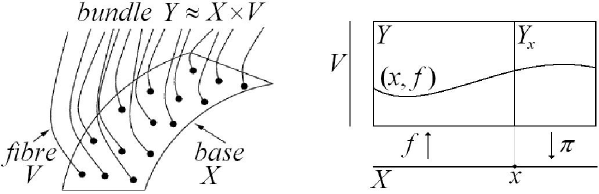
Figure 1: A sketch of a locally trivial fibre bundle $Y\approx X\times V$ as a generalization of a product space $X\times V$; left – main components; right – a few details (see text for explanation).

More generally, a biomechanical configuration bundle, $\pi:Y\allowbreak\mathrel{\mathop{\hbox to11.99998pt{\rightarrowfill}}\limits}X$, is a locally trivial fibred (or, projection) manifold over the base $X$. It is endowed with an atlas of fibred bundle coordinates $(x^{\lambda},y^{i})$, where $(x^{\lambda})$ are coordinates of $X$.

A linear connection $\bar{\Gamma}$ on a biomechanical bundle $Y\allowbreak\mathrel{\mathop{\hbox to11.99998pt{\rightarrowfill}}\limits}X$ is given in local coordinates on $Y$ by [14]

$$\bar{\Gamma}=dx^{\lambda}\otimes[\partial_{\lambda}-\Gamma^{i}{}_{j\lambda}(x)y^{j}\partial_{i}].$$ (14)

An affine connection $\Gamma$ on a biomechanical bundle $Y\allowbreak\mathrel{\mathop{\hbox to11.99998pt{\rightarrowfill}}\limits}X$ is given in local coordinates on $Y$ by

$$\Gamma=dx^{\lambda}\otimes[\partial_{\lambda}+(-\Gamma^{i}{}_{j\lambda}(x)y^{j}+\Gamma^{i}{}_{\lambda}(x))\partial_{i}].$$

Clearly, a linear connection $\bar{\Gamma}$ is a special case of an affine connection $\Gamma$.

Every connection $\Gamma$ on a biomechanical bundle $Y\allowbreak\mathrel{\mathop{\hbox to11.99998pt{\rightarrowfill}}\limits}X$ defines a system of first–order differential equations on $Y$, given by the local coordinate relations

$$y^{i}_{\lambda}=\Gamma^{i}(y).$$ (15)

Integral sections for $\Gamma$ are local solutions of (15).

4.2 Biomechanical Jets

A pair of smooth manifold maps,  $f_{1},f_{2}:M\rightarrow N$  (see Figure 2), are said to be $k-$tangent (or tangent of order $k$, or have a $k$th order contact) at a point $x$ on a domain manifold $M$, denoted by $f_{1}\sim f_{2}$, iff

$$f_{1}(x) = f_{2}(x)\qquad\text{called}\quad 0-\text{tangent},$$

$$\partial_{x}f_{1}(x) = \partial_{x}f_{2}(x),\qquad\text{called}\quad 1-\text{tangent},$$

$$\partial_{xx}f_{1}(x) = \partial_{xx}f_{2}(x),\qquad\text{called}\quad 2-\text{tangent},$$

$$...\qquad\text{etc. to the order }k$$

In this way defined $k-$tangency is an equivalence relation.

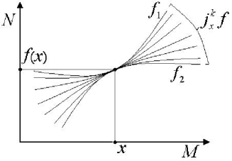
Figure 2: An intuitive geometrical picture behind the $k-$jet concept, based on the idea of a higher–order tangency (or, higher–order contact).

A $k-$jet (or, a jet of order $k$), denoted by $j_{x}^{k}f$, of a smooth map $f:M\rightarrow N$ at a point $x\in M$ (see Figure 2), is defined as an equivalence class of $k-$tangent maps at $x$,

$$j_{x}^{k}f:M\rightarrow N=\{f^{\prime}:f^{\prime}\text{ is }k-\text{tangent to }f\text{ at }x\}.$$

For example, consider a simple function  $f:X\rightarrow Y,\,x\mapsto y=f(x)$, mapping the $X-$axis into the $Y-$axis in $\mathbb{R}^{2}$. At a chosen point $x\in X$ we have:
a $0-$jet is a graph: $(x,f(x))$;
a $1-$jet is a triple: $(x,f(x),f{{}^{\prime}}(x))$;
a $2-$jet is a quadruple: $(x,f(x),f{{}^{\prime}}(x),f^{\prime\prime}(x))$,
   and so on, up to the order $k$ (where $f{{}^{\prime}}(x)=\frac{df(x)}{dx}$, etc).
The set of all $k-$jets from $j^{k}_{x}f:X\rightarrow Y$ is called the $k-$jet manifold $J^{k}(X,Y)$.

Formally, given a biomechanical bundle $Y\allowbreak\mathrel{\mathop{\hbox to11.99998pt{\rightarrowfill}}\limits}X$, its first–order jet manifold $J^{1}Y$ comprises the set of equivalence classes $j^{1}_{x}s$, $x\in X$, of sections $s:X\allowbreak\mathrel{\mathop{\hbox to11.99998pt{\rightarrowfill}}\limits}Y$ so that sections $s$ and $s^{\prime}$ belong to the same class iff

$$Ts\mid_{T_{x}X}=Ts^{\prime}\mid_{T_{x}X}.$$

Intuitively, sections $s,s^{\prime}\in j^{1}_{x}s$ are identified by their values $s^{i}(x)={s^{\prime}}^{i}(x)$ and the values of their partial derivatives $\partial_{\mu}s^{i}(x)=\partial_{\mu}{s^{\prime}}^{i}(x)$ at the point $x$ of $X$. There are the natural fibrations [14]

$$\pi_{1}:J^{1}Y\ni j^{1}_{x}s\mapsto x\in X,\qquad\pi_{01}:J^{1}Y\ni j^{1}_{x}s\mapsto s(x)\in Y.$$

Given bundle coordinates $(x^{\lambda},y^{i})$ of $Y$, the associated jet manifold $J^{1}Y$ is endowed with the adapted coordinates

$$(x^{\lambda},y^{i},y_{\lambda}^{i}),\qquad(y^{i},y_{\lambda}^{i})(j^{1}_{x}s)=(s^{i}(x),\partial_{\lambda}s^{i}(x)),\qquad{y^{\prime}}^{i}_{\lambda}=\frac{\partial x^{\mu}}{\partial{x^{\prime}}^{\lambda}}(\partial_{\mu}+y^{j}_{\mu}\partial_{j})y^{\prime i}.$$

In particular, given the biomechanical configuration bundle $M\rightarrow\mathbb{R}$ over the time axis $\mathbb{R}$, the $1-$jet space $J^{1}(\mathbb{R},M)$ is the set of equivalence classes $j_{t}^{1}s$ of sections $s^{i}:\mathbb{R}\rightarrow M$ of the configuration bundle $M\rightarrow\mathbb{R}$, which are identified by their values $s^{i}(t)$, as well as by the values of their partial derivatives $\partial_{t}s^{i}=\partial_{t}s^{i}(t)$ at time points $t\in\mathbb{R}$. The 1–jet manifold $J^{1}(\mathbb{R},M)$ is coordinated by $(t,x^{i},\dot{x}^{i})$, that is by (time, coordinates and velocities) at every active human joint, so the 1–jets are local joint coordinate maps

$$j_{t}^{1}s:\mathbb{R}\rightarrow M,\qquad t\mapsto(t,x^{i},\dot{x}^{i}).$$

The repeated jet manifold $J^{1}J^{1}Y$ is defined to be the jet manifold of the bundle $J^{1}Y\allowbreak\mathrel{\mathop{\hbox to11.99998pt{\rightarrowfill}}\limits}X$. It is endowed with the adapted coordinates $(x^{\lambda},y^{i},y^{i}_{\lambda},y_{(\mu)}^{i},y^{i}_{\lambda\mu})$.

The second–order jet manifold $J^{2}Y$ of a bundle $Y\allowbreak\mathrel{\mathop{\hbox to11.99998pt{\rightarrowfill}}\limits}X$ is the subbundle of $\widehat{J}^{2}Y\allowbreak\mathrel{\mathop{\hbox to11.99998pt{\rightarrowfill}}\limits}J^{1}Y$ defined by the coordinate conditions $y^{i}_{\lambda\mu}=y^{i}_{\mu\lambda}$. It has the local coordinates $(x^{\lambda},y^{i},y^{i}_{\lambda},y^{i}_{\lambda\leq\mu})$ together with the transition functions [14]

$${y^{\prime}}_{\lambda\mu}^{i}=\frac{\partial x^{\alpha}}{\partial{x^{\prime}}^{\mu}}(\partial_{\alpha}+y^{j}_{\alpha}\partial_{j}+y^{j}_{\nu\alpha}\partial^{\nu}_{j}){y^{\prime}}^{i}_{\lambda}.$$

The second–order jet manifold $J^{2}Y$ of $Y$ comprises the equivalence classes $j_{x}^{2}s$ of sections $s$ of
$Y\allowbreak\mathrel{\mathop{\hbox to11.99998pt{\rightarrowfill}}\limits}X$ such that

$$y^{i}_{\lambda}(j_{x}^{2}s)=\partial_{\lambda}s^{i}(x),\qquad y^{i}_{\lambda\mu}(j_{x}^{2}s)=\partial_{\mu}\partial_{\lambda}s^{i}(x).$$

In other words, two sections $s,s^{\prime}\in j^{2}_{x}s$ are identified by their values and the values of their first and second–order derivatives at the point $x\in X$.

In particular, given the biomechanical configuration bundle $M\rightarrow\mathbb{R}$ over the time axis $\mathbb{R}$, the $2-$jet space $J^{2}(\mathbb{R},M)$ is the set of equivalence classes $j_{t}^{2}s$ of sections $s^{i}:\mathbb{R}\rightarrow M$ of the configuration bundle $\pi:M\rightarrow\mathbb{R}$, which are identified by their values $s^{i}(t)$, as well as the values of their first and second partial derivatives, $\partial_{t}s^{i}=\partial_{t}s^{i}(t)$ and $\partial_{tt}s^{i}=\partial_{tt}s^{i}(t)$, respectively, at time points $t\in\mathbb{R}$. The 2–jet manifold $J^{2}(\mathbb{R},M)$ is coordinated by $(t,x^{i},\dot{x}^{i},\ddot{x}^{i})$, that is by (time, coordinates, velocities and accelerations) at every active human joint, so the 2–jets are local joint coordinate maps

$$j_{t}^{2}s:\mathbb{R}\rightarrow M,\qquad t\mapsto(t,x^{i},\dot{x}^{i},\ddot{x}^{i}).$$

4.3 Polysymplectic Dynamics

Let $Y\allowbreak\mathrel{\mathop{\hbox to11.99998pt{\rightarrowfill}}\limits}X$ be a biomechanical bundle with local coordinates $(x^{\lambda},y^{i})$. In jet terms, a first–order Lagrangian is defined (through the standard Lagrangian density ${\cal L}$) to be a horizontal density $L={\cal L}\omega$ on the jet manifold $J^{1}Y$. The jet manifold $J^{1}Y$ plays the role of the finite-dimensional configuration space of sections of the bundle $Y\allowbreak\mathrel{\mathop{\hbox to11.99998pt{\rightarrowfill}}\limits}X$.

Lagrangian $L$ yields the Legendre morphism $\widehat{L}:J^{1}Y\allowbreak\mathrel{\mathop{\hbox to11.99998pt{\rightarrowfill}}\limits}\Pi$, from the 1–jet manifold $J^{1}Y$ to the Legendre manifold, given by a product [14]

$$\Pi=V^{*}Y\mathop{\wedge}\limits(\mathop{\wedge}\limits^{n-1}T^{*}X)=V^{*}Y\mathop{\wedge}\limits(\mathop{\wedge}\limits^{n}T^{*}X)\mathop{\otimes}\limits TX,$$ (16)

where $V$ is called the vertical bundle. $\Pi$ plays the role of the finite-dimensional phase-space of sections of $Y\allowbreak\mathrel{\mathop{\hbox to11.99998pt{\rightarrowfill}}\limits}X$. Given the bundle coordinates $(x^{\lambda},y^{i})$ on $Y\allowbreak\mathrel{\mathop{\hbox to11.99998pt{\rightarrowfill}}\limits}X$, the Legendre bundle (16) has local coordinates $(x^{\lambda},y^{i},p^{\lambda}_{i})$, where $p^{\lambda}_{i}$ are the holonomic coordinates with the transition functions

$${p^{\prime}}^{\lambda}_{i}=\det(\frac{\partial x^{\varepsilon}}{\partial{x^{\prime}}^{\nu}})\frac{\partial y^{j}}{\partial{y^{\prime}}^{i}}\frac{\partial{x^{\prime}}^{\lambda}}{\partial x^{\mu}}p^{\mu}_{j}.$$ (17)

Relative to these coordinates, the Legendre morphism $\widehat{L}$ reads

$$p^{\mu}_{i}\circ\widehat{L}=\pi^{\mu}_{i}.$$ (18)

The Legendre manifold $\Pi$ in (16) is equipped with the generalized Liouville form

$${\Theta}=-p^{\lambda}_{i}dy^{i}\wedge\omega\otimes\partial_{\lambda},$$ (19)

where $\otimes$ denotes the standard tensor product. Furthermore, for any Pfaffian form $\theta$ on $X$ we have the relation

$${\Lambda}\rfloor\theta=-d({\Theta}\rfloor\theta).$$

This relation introduces the the canonical polysymplectic form on the Legendre manifold $\Pi$,

$${\Lambda}=dp^{\lambda}_{i}\wedge dy^{i}\wedge\omega\otimes\partial_{\lambda},$$ (20)

whose coordinate expression (20) is maintained under holonomic coordinate transformations (17). It is a pullback-valued form [14].

4.4 Hamiltonian Connections

Let $J^{1}\Pi$ be the jet manifold of the Legendre bundle $\Pi\allowbreak\mathrel{\mathop{\hbox to11.99998pt{\rightarrowfill}}\limits}X$. It is endowed with the adapted coordinates $(x^{\lambda},y^{i},p^{\lambda}_{i},y^{i}_{\mu},p^{\lambda}_{i\mu})$. By analogy with the notion of an autonomous Hamiltonian vector-field $X_{H}$ in (5), a connection $\gamma$ on the bundle $\Pi\allowbreak\mathrel{\mathop{\hbox to11.99998pt{\rightarrowfill}}\limits}X$, given by

$$\gamma=dx^{\lambda}\otimes(\partial_{\lambda}+\gamma^{i}_{\lambda}\partial_{i}+\gamma^{\mu}_{i\lambda}\partial^{i}_{\mu}),$$

is said to be locally Hamiltonian if the exterior form $\gamma\rfloor{\Lambda}$ is closed and Hamiltonian if the form $\gamma\rfloor{\Lambda}$ is exact. A connection $\gamma$ is locally Hamiltonian iff it obeys the conditions [14, 15]

$$\partial^{i}_{\lambda}\gamma^{j}_{\mu}-\partial^{j}_{\mu}\gamma^{i}_{\lambda}=0,\quad\partial_{i}\gamma_{j\mu}^{\mu}-\partial_{j}\gamma_{i\mu}^{\mu}=0,\quad\partial_{j}\gamma_{\lambda}^{i}+\partial_{\lambda}^{i}\gamma_{j\mu}^{\mu}=0.$$ (21)

A $p-$form $H$ on the Legendre bundle $\Pi\allowbreak\mathrel{\mathop{\hbox to11.99998pt{\rightarrowfill}}\limits}X$ is called a general Hamiltonian form if there exists a Hamiltonian connection such that

$$\gamma\rfloor{\Lambda}=dH.$$

A general, dissipative, time-dependent Hamiltonian form $H$ on $\Pi$ is said to be Hamiltonian if it has the splitting

$$H=H_{\Gamma}-\widetilde{H}_{\Gamma}=p^{\lambda}_{i}dy^{i}\wedge\omega_{\lambda}-(p^{\lambda}_{i}\Gamma^{i}_{\lambda}+\widetilde{{\cal H}}_{\Gamma})\omega=p^{\lambda}_{i}dy^{i}\wedge\omega_{\lambda}-{\cal H}\omega$$ (22)

modulo closed forms, where $\Gamma$ is a connection on $Y$ and $\widetilde{H}_{\Gamma}$ is a horizontal density. This splitting is preserved under the holonomic coordinate transformations (17).

Let a Hamiltonian connection $\gamma$ associated with a Hamiltonian form $H$ have an integral section $s$ of $\Pi\allowbreak\mathrel{\mathop{\hbox to11.99998pt{\rightarrowfill}}\limits}X$, that is, $\gamma\circ s=J^{1}s$. Then $s$ satisfies the system of first–order Hamiltonian equations on $\Pi$,

$$y^{i}_{\lambda}=\partial^{i}_{\lambda}{\cal H},\qquad p^{\lambda}_{i\lambda}=-\partial_{i}{\cal H}.$$

4.5 Time–Dependent Dissipative Hamiltonian Dynamics

We can now formulate the time-dependent biomechanics as an $n=1-$reduction of polysymplectic dynamics described above. The biomechanical phase space is the Legendre manifold $\Pi$, endowed with the holonomic coordinates $(t,y^{i},p_{i})$ with the transition functions

$$p^{\prime}_{i}=\frac{\partial y^{j}}{\partial{y^{\prime}}^{i}}p_{j}.$$

$\Pi$ admits the canonical form ${\Lambda}$ (20), which now reads

$${\Lambda}=dp_{i}\wedge dy^{i}\wedge dt\otimes\partial_{t}.$$

As a particular case of the polysymplectic machinery of the previous section, we say that a connection

$$\gamma=dt\otimes(\partial_{t}+\gamma^{i}\partial_{i}+\gamma_{i}\partial^{i})$$

on the bundle $\Pi\allowbreak\mathrel{\mathop{\hbox to11.99998pt{\rightarrowfill}}\limits}X$ is locally Hamiltonian if the exterior form $\gamma\rfloor{\Lambda}$ is closed and Hamiltonian if the form $\gamma\rfloor{\Lambda}$ is exact. A connection $\gamma$ is locally Hamiltonian iff it obeys the conditions (21) which now take the form

$$\partial^{i}\gamma^{j}-\partial^{j}\gamma^{i}=0,\quad\partial_{i}\gamma_{j}-\partial_{j}\gamma_{i}=0,\quad\partial_{j}\gamma^{i}+\partial^{i}\gamma_{j}=0.$$

Note that every connection $\Gamma=dt\otimes(\partial_{t}+\Gamma^{i}\partial_{i})$ on the bundle $Y\allowbreak\mathrel{\mathop{\hbox to11.99998pt{\rightarrowfill}}\limits}X$ gives rise to the Hamiltonian connection $\widetilde{\Gamma}$ on $\Pi\allowbreak\mathrel{\mathop{\hbox to11.99998pt{\rightarrowfill}}\limits}X$, given by

$$\widetilde{\Gamma}=dt\otimes(\partial_{t}+\Gamma^{i}\partial_{i}-\partial_{j}\Gamma^{i}p_{i}\partial^{j}).$$

The corresponding Hamiltonian form $H_{\Gamma}$ is given by

$$H_{\Gamma}=p_{i}dy^{i}-p_{i}\Gamma^{i}dt.$$

Let $H$ be a dissipative Hamiltonian form (22) on $\Pi$, which reads:

$$H=p_{i}dy^{i}-{\cal H}dt=p_{i}dy^{i}-p_{i}\Gamma^{i}dt-\widetilde{{\cal H}}_{\Gamma}dt.$$ (23)

We call ${\cal H}$ and $\widetilde{\cal H}$ in the decomposition (23) the Hamiltonian and the Hamiltonian function respectively. Let $\gamma$ be a Hamiltonian connection on $\Pi\allowbreak\mathrel{\mathop{\hbox to11.99998pt{\rightarrowfill}}\limits}X$ associated with the Hamiltonian form (23). It satisfies the relations [14, 15]

$$\gamma\rfloor{\Lambda}=dp_{i}\wedge dy^{i}+\gamma_{i}dy^{i}\wedge dt-\gamma^{i}dp_{i}\wedge dt=dH,$$

$$\gamma^{i}=\partial^{i}{\cal H},\qquad\gamma_{i}=-\partial_{i}{\cal H}.$$ (24)

From equations (24) we see that, in the case of biomechanics, one and only one Hamiltonian connection is associated with a given Hamiltonian form.

Every connection $\gamma$ on $\Pi\allowbreak\mathrel{\mathop{\hbox to11.99998pt{\rightarrowfill}}\limits}X$ yields the system of first–order differential equations (15), which now takes the explicit form:

$$\dot{y}^{i}=\gamma^{i},\qquad\dot{p}_{i}=\gamma_{i}.$$ (25)

They are called the evolution equations. If $\gamma$ is a Hamiltonian connection associated with the Hamiltonian form $H$ (23), the evolution equations (25) become the dissipative time-dependent Hamiltonian equations:

$$\dot{y}^{i}=\partial^{i}{\cal H},\qquad\dot{p}_{i}=-\partial_{i}{\cal H}.$$ (26)

In addition, given any scalar function $f$ on $\Pi$, we have the dissipative Hamiltonian evolution equation

$$d_{H}f=(\partial_{t}+\partial^{i}{\cal H}\partial_{i}-\partial_{i}{\cal H}\partial^{i})\,f,$$ (27)

relative to the Hamiltonian ${\cal H}$. On solutions $s$ of the Hamiltonian equations (26), the evolution equation (27) is equal to the total time derivative of the function $f$:

$$s^{*}d_{H}f=\frac{d}{dt}(f\circ s).$$

4.6 Time & Fitness–Dependent Biomechanics

The dissipative Hamiltonian system (26)–(27) is the basis for our time & fitness-dependent biomechanics. The scalar function $f$ in (27) on the biomechanical Legendre phase-space manifold $\Pi$ is now interpreted as an individual neuro-muscular fitness function. This fitness function is a ‘determinant’ for the performance of muscular drives for the driven, dissipative Hamiltonian biomechanics. These muscular drives, for all active DOF, are given by time & fitness-dependent Pfaffian form: $F_{i}=F_{i}(t,y,p,f)$. In this way, we obtain our final model for time & fitness-dependent Hamiltonian biomechanics:

$$\dot{y}^{i} = \partial^{i}{\cal H},$$

$$\dot{p}_{i} = F_{i}-\partial_{i}{\cal H},$$

$$d_{H}f = (\partial_{t}+\partial^{i}{\cal H}\partial_{i}-\partial_{i}{\cal H}\partial^{i})\,f.$$

Physiologically, the active muscular drives $F_{i}=F_{i}(t,y,p,f)$ consist of [1, 2]):

1. Synovial joint mechanics, giving the first stabilizing effect to the conservative skeleton dynamics, is described by the $(y,\dot{y})$–form of the Rayleigh–Van der Pol’s dissipation function

$$R=\frac{1}{2}\sum_{i=1}^{n}\,(\dot{y}^{i})^{2}\,[\alpha_{i}\,+\,\beta_{i}(y^{i})^{2}],\quad$$

where $\alpha_{i}$ and $\beta_{i}$ denote dissipation parameters. Its partial derivatives give rise to the viscous–damping torques and forces in the joints

$$\mathcal{F}_{i}^{joint}=\partial R/\partial\dot{y}^{i},$$

which are linear in $\dot{y}^{i}$ and quadratic in $y^{i}$.

2. Muscular mechanics, giving the driving torques and forces $\mathcal{F}_{i}^{musc}=\mathcal{F}_{i}^{musc}(t,y,\dot{y})$ with $(i=1,\dots,n)$ for human biomechanics, describes the internal excitation and contraction dynamics of equivalent muscular actuators [11].

(a) The excitation dynamics can be described by an impulse force–time relation

$$F_{i}^{imp} = F_{i}^{0}(1\,-\,e^{-t/\tau_{i}})\text{ \qquad if stimulation }>0$$

$$\quad F_{i}^{imp} = F_{i}^{0}e^{-t/\tau_{i}}\qquad\qquad\;\quad\text{if stimulation }=0,\quad$$

where $F_{i}^{0}$ denote the maximal isometric muscular torques and forces, while $\tau_{i}$ denote the associated time characteristics of particular muscular actuators. This relation represents a solution of the Wilkie’s muscular active–state element equation [12]

$$\dot{\mu}\,+\,\Gamma\,\mu\,=\,\Gamma\,S\,A,\quad\mu(0)\,=\,0,\quad 0<S<1,$$

where $\mu=\mu(t)$ represents the active state of the muscle, $\Gamma$ denotes the element gain, $A$ corresponds to the maximum tension the element can develop, and $S=S(r)$ is the ‘desired’ active state as a function of the motor unit stimulus rate $r$. This is the basis for biomechanical force controller.

(b) The contraction dynamics has classically been described by the Hill’s hyperbolic force–velocity relation [13]

$$F_{i}^{Hill}\,=\,\frac{\left(F_{i}^{0}b_{i}\,-\,\delta_{ij}a_{i}\dot{y}^{j}\,\right)}{\left(\delta_{ij}\dot{y}^{j}\,+\,b_{i}\right)},\,\quad$$

where $a_{i}$ and $b_{i}$ denote the Hill’s parameters, corresponding to the energy dissipated during the contraction and the phosphagenic energy conversion rate, respectively, while $\delta_{ij}$ is the Kronecker’s $\delta-$tensor.

In this way, human biomechanics describes the excitation/contraction dynamics for the $i$th equivalent muscle–joint actuator, using the simple impulse–hyperbolic product relation

$$\mathcal{F}_{i}^{musc}(t,y,\dot{y})=\,F_{i}^{imp}\times F_{i}^{Hill}.\quad$$

Now, for the purpose of biomedical engineering and rehabilitation, human biomechanics has developed the so–called hybrid rotational actuator. It includes, along with muscular and viscous forces, the D.C. motor drives, as used in robotics

$$\mathcal{F}_{k}^{robo}=i_{k}(t)-J_{k}\ddot{y}_{k}(t)-B_{k}\dot{y}_{k}(t),\qquad\text{with}$$

$$l_{k}i_{k}(t)+R_{k}i_{k}(t)+C_{k}\dot{y}_{k}(t)=u_{k}(t),$$

where $k=1,\dots,n$, $i_{k}(t)$ and $u_{k}(t)$ denote currents and voltages in the rotors of the drives, $R_{k},l_{k}$ and $C_{k}$ are resistances, inductances and capacitances in the rotors, respectively, while $J_{k}$ and $B_{k}$ correspond to inertia moments and viscous dampings of the drives, respectively.

Finally, to make the model more realistic, we need to add some stochastic torques and forces:

$$\mathcal{F}_{i}^{stoch}=B_{ij}[y^{i}(t),t]\,dW^{j}(t),$$

where $B_{ij}[y(t),t]$ represents continuous stochastic diffusion fluctuations, and $W^{j}(t)$ is an $N-$variable Wiener process (i.e., generalized Brownian motion) [5], with

$$dW^{j}(t)=W^{j}(t+dt)-W^{j}(t),\qquad(\text{for}~{}~{}j=1,\dots,n=\text{no. of active DOF}).$$

5 Conclusion

We have presented the time-dependent generalization of an ‘ordinary’ autonomous Hamiltonian biomechanics, in which total mechanical + biochemical energy is not conserved. Starting with the Covariant Force Law, we have first developed autonomous Hamiltonian biomechanics. Then we have introduced a general framework for time-dependent Hamiltonian biomechanics in terms jets, Legendre manifolds and dissipative Hamiltonian connections associated with the extended musculo-skeletal configuration manifold, called the configuration bundle. In this way we formulated a general Hamiltonian model for time & fitness-dependent human biomechanics.

References

- [1] Ivancevic, V., Ivancevic, T., Human–Like Biomechanics: A Unified Mathematical Approach to Human Biomechanics and Humanoid Robotics. Springer, Dordrecht, (2006)
- [2] Ivancevic, V., Ivancevic, T., Natural Biodynamics. World Scientific, Singapore (2006)
- [3] Ivancevic, V., Ivancevic, T., Geometrical Dynamics of Complex Systems: A Unified Modelling Approach to Physics, Control, Biomechanics, Neurodynamics and Psycho-Socio-Economical Dynamics. Springer, Dordrecht, (2006)
- [4] Ivancevic, V., Ivancevic, T., Applied Differential Geometry: A Modern Introduction. World Scientific, Singapore, (2007)
- [5] Ivancevic, V., Ivancevic, T., High–Dimensional Chaotic and Attractor Systems. Springer, Berlin, (2006)
- [6] Ivancevic, V., Ivancevic, T., Human versus humanoid robot biodynamcis. Int. J. Hum. Rob. 5(4), 699 -713, (2008)
- [7] Ivancevic, V., Ivancevic, T., Complex Nonlinearity: Chaos, Phase Transitions, Topology Change and Path Integrals, Springer, Berlin, (008)
- [8] Ivancevic, T., Jovanovic, B., Djukic, M., Markovic, S., Djukic, N., Biomechanical Analysis of Shots and Ball Motion in Tennis and the Analogy with Handball Throws, J. Facta Universitatis, Series: Sport, 6(1), 51–66, (2008)
- [9] Ivancevic, T., Jain, L., Pattison, J., Hariz, A., Nonlinear Dynamics and Chaos Methods in Neurodynamics and Complex Data Analysis, Nonl. Dyn. (Springer), 56(1-2), 23–44, (2009)
- [10] Ivancevic, T., Jovanovic, B., Djukic, S., Djukic, M., Markovic, S., Complex Sports Biodynamics: With Practical Applications in Tennis, Springer, Berlin, (2009)
- [11] Hatze, H., A general myocybernetic control model of skeletal muscle. Biol. Cyber. 28, 143–157, (1978)
- [12] Wilkie, D.R., The mechanical properties of muscle. Brit. Med. Bull. 12, 177–182, (1956)
- [13] Hill, A.V.,The heat of shortening and the dynamic constants of muscle. Proc. Roy. Soc. B76, 136–195, (1938)
- [14] Giachetta, G., Mangiarotti, L., Sardanashvily, G., New Lagrangian and Hamiltonian Methods in Field Theory, World Scientific, Singapore, (1997)
- [15] Sardanashvily, G.: Hamiltonian time-dependent mechanics. J. Math. Phys. 39, 2714, (1998)