Exact Solution of the Discrete (1+1)–dimensional RSOS Model with Field and Surface Interactions

Abstract

We present the solution of a linear Restricted Solid–on–Solid (RSOS) model in a field. Aside from the origins of this model in the context of describing the phase boundary in a magnet, interest also comes from more recent work on the steady state of non-equilibrium models of molecular motors.

While similar to a previously solved (non-restricted) SOS model in its physical behaviour, mathematically the solution is more complex. Involving basic hypergeometric functions ${}_{3}\phi_{2}$, it introduces a new form of solution to the lexicon of directed lattice path generating functions.

1 Introduction

The SOS model arose from the consideration of the boundary between oppositely magnetised phases in the Ising model [1] at low temperatures and is now considered to be useful for describing the salient features of a wide variety of interfacial phenomena [2, 3, 4, 5, 6]. The configurations involved in the linear (1+1)–dimensional case, modelling the interface in a two-dimensional magnet, have also been used to model the backbone of a polymer in solution. The critical phenomena associated with this model describe wetting transitions of the interface with a wall [2]. For the SOS model the phase diagram contains a wetting transition at finite temperature $T_{w}$ for zero field and complete wetting occurs taking the limit $H\to 0$ for $T\geq T_{w}$ [7].

The linear SOS model with magnetic field and wall interaction was solved in [7]. The restricted SOS model is a variant of the SOS model where the interface takes on a restricted subset of configurations as opposed to the full SOS model. Effectively it suppresses very large local fluctuations of the interface. This model has been considered with wall interaction, but not yet with magnetic field. This is partially because, with wall interaction only, the SOS and RSOS models are in the same universality class, as demonstrated by their exact solutions [8, 9, 10, 11, 12, 13]. Recently, it has been suggested that the RSOS model in a field describes the steady state of a non-equilibrium model of a molecular motor [14]. This observation has motivated us to consider the RSOS model in a field. In doing so, we have discovered a novel form of generating function for a directed lattice path problem, and a new method of solution for such problems.

The RSOS model we analyse can be described as follows. Consider a two-dimensional square lattice in a half plane. For each column $i$ of the surface a segment of the interface is placed on the horizontal link at height $r_{i}\geq 0$ and successive segments are joined by vertical segments to form a partially directed interface with no overhangs. The configurations are given the energy

$$-\beta E=-K\sum_{i}|r_{i}-r_{i-1}|-H\sum_{i}r_{i}+b\sum_{i}\delta_{r_{i},0}\;.$$ (1.1)

There are two basic variants of this model which have been discussed in the literature. If there are no restrictions placed on the differences of successive heights $r_{i}$, the model is called the (unrestricted) SOS model, analysed in [7].

On the other hand, constraining the height differences to be bounded by

$$|\Delta r_{i}|=|r_{i}-r_{i-1}|\leq 1$$ (1.2)

gives the restricted SOS (RSOS) model. This has previously only been considered in the case of zero field $H$ [8, 9], for several types of external potential [15]. Both variants have been considered, utilising a different thermodynamic ensemble, as models for polymers in solution, since the finite configurations are partially directed self-avoiding walks [8, 16]. In [17] a RSOS model with $H=0$ but a rigidity term dependent on $|\Delta r_{i}-\Delta r_{i-1}|$ has been considered as a model of semi-flexible polymers such as DNA.

2 The RSOS generating function

We discuss the RSOS model in terms of lattice paths. An RSOS path is a partially directed self-avoiding path with no steps into the negative $x$-direction and no successive vertical steps. To be precise, an RSOS path of width $N$ with heights $r_{0}$ to $r_{N}$ has horizontal steps at heights $r_{1},\ldots,r_{N}$, and vertical steps between heights $r_{i-1}$ and $r_{i}$ for $i=1,\ldots,N$, but no horizontal step associated with $r_{0}$. This means that an RSOS path starts at height $r_{0}$ with either a horizontal step (if $r_{1}=r_{0}$) or vertical step (if $r_{1}\neq r_{0}$), but must end at height $r_{N}$ with a horizontal step. Figure 1 shows an example.

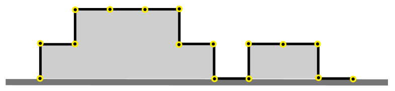
Figure 1: A typical RSOS configuration beginning on the surface and finishing on the surface with a horizontal step: each horizontal step is assigned a weight $x$, each vertical step a weight $y$, each unit of area a weight $q$, and each step that touches the surface an additional weight $\kappa$. The width of the configuration shown here is $N=9$, and the heights are $r_{0}=0$, $r_{1}=1$, $r_{2}=r_{3}=r_{4}=2$, $r_{5}=1$, $r_{6}=0$, $r_{7}=r_{8}=1$, and $r_{9}=0$. The weight of this configuration equals $x^{9}y^{6}q^{10}\kappa^{2}$.

The partition function for the RSOS paths of width $N$ with ends fixed at heights $r_{0}\geq 0$ and $r_{N}\geq 0$, respectively, is given by

$$Z_{1}(r_{0};r_{1})=\begin{cases}\exp(-\beta E(r_{0};r_{1}))\;,&|r_{0}-r_{1}|\leq 1\\ 0\;,&|r_{0}-r_{1}|>1\;,\end{cases}$$ (2.1)

and

$$Z_{N}(r_{0};r_{N})=\sum_{\begin{subarray}{c}r_{1},\ldots,r_{N-1}\geq 0\\ |r_{i}-r_{i-1}|\leq 1\end{subarray}}\exp(-\beta E(r_{0};r_{1},\ldots,r_{N}))\;,\qquad N=2,3,\ldots\;,$$ (2.2)

where

$$-\beta E(r_{0};r_{1},\ldots,r_{N})=-K\sum_{i=1}^{N}|r_{i}-r_{i-1}|-H\sum_{i=1}^{N}r_{i}+b\sum_{i=1}^{N}\delta_{r_{i},0}\;.$$ (2.3)

Here, we shall consider paths with both ends attached to the surface, i.e. we shall focus on the partition function

$$Z_{N}=Z_{N}(0;0)\;.$$ (2.4)

We define

$$y=\exp(-K)\;,\quad q=\exp(-H)\;,\quad\mbox{and}\quad\kappa=\exp(b)\;,$$ (2.5)

so $y$ is a temperature–like, $q$ a magnetic field–like and $\kappa$ a binding energy–like variable, and write

$$Z_{N}=Z_{N}(y,q,\kappa)\;.$$ (2.6)

The free energy is then

$$-\beta f(y,q,\kappa)=\lim_{N\to\infty}\frac{1}{N}\log Z_{N}(y,q,\kappa)\;.$$ (2.7)

Define the generalised (grand canonical) partition function, or simply generating function, as

$$G(x,y,q,\kappa)=1+\sum_{N=1}^{\infty}x^{N}Z_{N}(y,q,\kappa)\;.$$ (2.8)

Thus, the radius of convergence $x_{c}(y,q,\kappa)$ of $G(x,y,q,\kappa)$ with respect to the series expansion in $x$ can be identified as $\exp(\beta f(y,q,\kappa))$, hence

$$f(y,q,\kappa)=kT\log x_{c}(y,q,\kappa)\;.$$ (2.9)

It is convenient to consider $G$ as a combinatorial generating function for RSOS paths, where $x$, $y$, $q$ and $\kappa$ are counting variables for appropriate properties of those paths. Interpreted in such a way, $x$ and $y$ are the weights of horizontal and vertical steps, respectively, $q$ is the weight for each unit of area enclosed by the RSOS path and the $x$-axis, and $\kappa$ is is an additional weight for each step that touches the surface. For example, the weight of the configuration in Figure 1 is $x^{9}y^{6}q^{10}\kappa^{2}$.

We find easily the first few terms of $G$ as a series expansion in $x$,

$$G(x,y,q,\kappa)=1+\kappa x+(\kappa^{2}+\kappa y^{2}q)x^{2}+\ldots\;,$$ (2.10)

where the constant term corresponds to a zero-step path starting and ending at height zero with weight one.

3 Functional equation and exact solution

The key to the solution is a combinatorial decomposition of RSOS paths which leads to a functional equation for the generating function $G$. This decomposition is done with respect to the left-most horizontal step touching the surface at height zero, and is shown diagrammatically in Figure 2.

Figure 2: The diagrammatic form of the functional equations for RSOS paths, indicating the combinatorial decomposition of RSOS paths.

We distinguish three cases:

• The RSOS path has zero width, and there is no horizontal step at height zero. The contribution to the generating function is $1$.

• The RSOS path starts with a horizontal step, which therefore is at height zero. The rest of this path is again a RSOS path. The contribution to the generating function is $\kappa xG(x,y,q,\kappa)$.

• The RSOS path starts with a vertical step. Then there will be a left-most horizontal step at height zero, and removing this step cuts the path into two pieces. The left path starts with a vertical and horizontal step, followed by an RSOS path starting and ending at height one and not touching the surface, followed by a vertical step to height zero. The right path is again a RSOS path. The contribution to the generating function is $yxqG(qx,y,q,1)y\kappa xG(x,y,q,\kappa)$.

Put together, this decomposition leads to a functional equation for the generating function

$$G(x,y,q,\kappa)=1+\kappa xG(x,y,q,\kappa)+\kappa x^{2}y^{2}qG(qx,y,q,1)G(x,y,q,\kappa)\;.$$ (3.1)

For $q=1$, the solution is a simple algebraic function

$$G(x,y,1,\kappa)=\left(1-\kappa x-\frac{\kappa}{2}\left(1-x-\sqrt{(1-x)^{2}-4x^{2}y^{2}}\right)\right)^{-1}\;,$$ (3.2)

and for general values of $q$, a formal iteration of (3.1) leads to a continued fraction expansion

$$G(x,y,q,\kappa)=\cfrac{1}{1-\kappa x-\cfrac{\kappa qx^{2}y^{2}}{1-qx-\cfrac{q^{3}x^{2}y^{2}}{1-q^{2}x-\cfrac{q^{5}x^{2}y^{2}}{1-q^{3}x-\cfrac{q^{7}x^{2}y^{2}}{1-q^{4}x-\ldots}}}}}\;.$$ (3.3)

However, there is a non-trivial method to solve the functional equation for $G$ in terms of power series. Our main result is an expression for $G$ involving $q$-series. In the next section, we shall derive the following expression:

$$G(x,y,q,1)=\frac{\alpha\,(\lambda qx;q)_{\infty}\phi\left[\lambda qx,q\frac{\lambda}{1-\lambda};q,q\right]+((1-\lambda)qx;q)_{\infty}\phi\left[(1-\lambda)qx,q\frac{1-\lambda}{\lambda};q,q\right]}{\alpha\,(\lambda x;q)_{\infty}\phi\left[\lambda x,q\frac{\lambda}{1-\lambda};q,q\right]+((1-\lambda)x;q)_{\infty}\phi\left[(1-\lambda)x,q\frac{1-\lambda}{\lambda};q,q\right]}$$ (3.4)

with

$$\alpha=\frac{\phi\left[0,q\frac{1-\lambda}{\lambda};q,q\right]-(1-\lambda)\phi\left[0,q\frac{1-\lambda}{\lambda};q,q^{2}\right]}{\lambda\phi\left[0,q\frac{\lambda}{1-\lambda};q,q^{2}\right]-\phi\left[0,q\frac{\lambda}{1-\lambda};q,q\right]}$$ (3.5)

and

$$y^{2}=\lambda(1-\lambda)\;.$$ (3.6)

Here $\phi$ is given in terms of the basic hypergeometric function ${}_{3}\phi_{2}$ as

$$\phi[s,t;q,z]={}_{3}\phi_{2}\left(\genfrac{}{}{0.0pt}{}{0,0,0}{s,t};q,z\right)=\sum_{n=0}^{\infty}\frac{z^{n}}{(s;q)_{n}(t;q)_{n}(q;q)_{n}}$$ (3.7)

and

$$(t;q)_{n}=\prod_{k=0}^{n-1}(1-tq^{k})$$ (3.8)

is the standard $q$-product. From Equation (3.1) we have the full solution as

$$G(x,y,q,\kappa)=\frac{1}{1-\kappa x-\kappa x^{2}y^{2}qG(qx,y,q,1)}\;.$$ (3.9)

4 Solving the functional equation

Using a linearisation Ansatz [18], standard for a $q$-deformed algebraic equation such as Equation (3.1), we substitute

$$G(x,y,q,1)=\frac{H(qx,y,q)}{H(x,y,q)}$$ (4.1)

into Equation (3.1) with $\kappa=1$, and find that $H(x,y,q)$ must satisfy the linear $q$-functional equation

$$H(x,y,q)+(x-1)H(qx,y,q)+qx^{2}y^{2}H(q^{2}x,y,q)=0\;.$$ (4.2)

We then try to solve this linear functional equation using a series in $x$,

$$H(x,y,q)=\sum_{n=0}^{\infty}c_{n}(y,q)x^{n}\;.$$ (4.3)

This unfortunately leads to a non-trivial three-term recurrence for the coefficients

$$(1-q^{n+2})c_{n+2}(y,q)+q^{n+1}c_{n+1}(y,q)+y^{2}q^{2n+1}c_{n}(y,q)=0$$ (4.4)

for $n\geq 0$ with initial condition $c_{0}(y,q)+(1-q)c_{1}(y,q)=0$. This is different from the two-term recurrences obtained when considering the models in [18] which can be solved by direct iteration.

Inspired by the structure of basic hypergeometric functions, which we know form the basis for a solution in the SOS model [7], we transform the coefficients as

$$c_{n}(y,q)=\frac{(-1)^{n}q^{n(n-1)/2}}{(q;q)_{n}}d_{n}(y,q)\;.$$ (4.5)

This leads to a recurrence

$$d_{n+2}(y,q)-d_{n+1}(y,q)+y^{2}d_{n}(y,q)=y^{2}q^{n+1}d_{n}(y,q)$$ (4.6)

for $n\geq 0$ with initial condition $d_{1}(y,q)=d_{0}(y,q)$. While this is still a three-term recurrence, only one of the terms has a non-constant coefficient.

The left-hand side of Equation (4.6) is a homogeneous difference equation with constant coefficients and characteristic polynomial

$$P(\lambda)=\lambda^{2}-\lambda+y^{2}\;.$$ (4.7)

If the right-hand side of Equation (4.6) were zero, the solution would be given as $d_{n}=A\lambda_{1}^{n}+B\lambda_{2}^{n}$ where $\lambda_{i}$ are the roots of $P(\lambda)=0$. To solve this recurrence, we use the Ansatz [8]

$$d_{n}(y,q)=\lambda^{n}\sum_{m=0}^{\infty}e_{m}(y,q,\lambda)q^{nm}\;.$$ (4.8)

Inserting this Ansatz into Equation (4.6) we find

$$P(\lambda)e_{0}(y,q,\lambda)+\sum_{m=1}^{\infty}q^{mn}\left[P(\lambda q^{m})e_{m}(y,q,\lambda)-y^{2}qe_{m-1}(y,q,\lambda)\right]=0\;.$$ (4.9)

Necessarily $P(\lambda)=0$, and normalising by letting $e_{0}(y,q,\lambda)=1$, we find by iteration

$$e_{m}(y,q,\lambda)=\frac{q^{m}}{(\lambda^{2}q/y^{2};q)_{m}(q;q)_{m}}\;.$$ (4.10)

The full solution to the recurrence equation (4.6) is a linear combination of (4.8) over both values of $\lambda$ satisfying $P(\lambda)=0$. If $P(\lambda)=0$, then also $P(y^{2}/\lambda)=0$, and we can write

$$d_{n}(y,q)=A\lambda^{n}\sum_{m=0}^{\infty}e_{m}(y,q,\lambda)q^{nm}+B(y^{2}/\lambda)^{n}\sum_{m=0}^{\infty}e_{m}(y,q,y^{2}/\lambda)q^{nm}\;,$$ (4.11)

where $\lambda$ is an arbitrarily chosen solution of $\lambda(1-\lambda)=y^{2}$. Using the initial condition $d_{0}(y,q)=d_{1}(y,q)$ we can solve for the ratio $\alpha=A/B$. We can somewhat simplify our expressions by noting that the dependence between $\lambda$ and $y$ implies that we can replace $y^{2}$ by $\lambda(1-\lambda)$. Noticing that the functions involved are ${}_{2}\phi_{1}$ basic hypergeometric series, we have

$$\alpha=\frac{{}_{2}\phi_{1}\left(\genfrac{}{}{0.0pt}{}{0,0}{q\frac{1-\lambda}{\lambda}};q,q\right)-(1-\lambda){}_{2}\phi_{1}\left(\genfrac{}{}{0.0pt}{}{0,0}{q\frac{1-\lambda}{\lambda}};q,q^{2}\right)}{\lambda{}_{2}\phi_{1}\left(\genfrac{}{}{0.0pt}{}{0,0}{q\frac{\lambda}{1-\lambda}};q,q^{2}\right)-{}_{2}\phi_{1}\left(\genfrac{}{}{0.0pt}{}{0,0}{q\frac{\lambda}{1-\lambda}};q,q\right)}$$ (4.12)

where

$${}_{2}\phi_{1}\left(\genfrac{}{}{0.0pt}{}{0,0}{s};q,z\right)=\sum_{n=0}^{\infty}\frac{z^{n}}{(s;q)_{n}(q;q)_{n}}={}_{3}\phi_{2}\left(\genfrac{}{}{0.0pt}{}{0,0,0}{0,s};q,z\right)\;.$$ (4.13)

Substituting the expression for $d_{n}$ given in (4.11) back into $H$ using Equations (4.5) and (4.3), we find that

$$H(x,y,q)= \alpha\sum_{m,n=0}^{\infty}\frac{q^{n(n-1)/2}(-\lambda x)^{n}q^{nm+m}}{(q\lambda/(1-\lambda);q)_{m}(q;q)_{m}(q;q)_{n}}$$ (4.14)

$$+\sum_{m,n=0}^{\infty}\frac{q^{n(n-1)/2}(-(1-\lambda)x)^{n}q^{nm+m}}{(q(1-\lambda)/\lambda;q)_{m}(q;q)_{m}(q;q)_{n}}\;.$$

The summation over $n$ can be done explicitly using Euler’s formula [19]

$$(t;q)_{\infty}=\sum_{n=0}^{\infty}\frac{q^{n(n-1)/2}(-t)^{n}}{(q;q)_{n}}\;.$$ (4.15)

We find that

$$H(x,y,q)=\alpha\sum_{m=0}^{\infty}\frac{(\lambda xq^{m};q)_{\infty}q^{m}}{(q\lambda/(1-\lambda);q)_{m}(q;q)_{m}}+\sum_{m=0}^{\infty}\frac{((1-\lambda)xq^{m};q)_{\infty}q^{m}}{(q(1-\lambda)/\lambda;q)_{m}(q;q)_{m}}$$ (4.16)

which after pulling out a $q$-product factor from each sum can be identified with

$$H(x,y,q)= \alpha\,(\lambda x;q)_{\infty}{}_{3}\phi_{2}\left(\genfrac{}{}{0.0pt}{}{0,0,0}{\lambda x,q\lambda/(1-\lambda)};q,q\right)$$ (4.17)

$$+((1-\lambda)x;q)_{\infty}{}_{3}\phi_{2}\left(\genfrac{}{}{0.0pt}{}{0,0,0}{(1-\lambda)x,q(1-\lambda)/\lambda};q,q\right)\;.$$

Substituting into the linearisation Ansatz (4.1) gives us the solution written in Equation (3.4).

5 Comparison of SOS and RSOS model solutions

The unrestricted SOS model was solved in [7] by a different technique, namely the Temperley method. For the sake of comparison it is worthwhile reproducing the solution of the SOS model via the functional equation technique presented above for the restricted SOS model. This highlights a fundamental difference in the difficulty of solving the two models.

In analogy to the functional equation (3.1), the SOS model generating function $S(x,y,q,\kappa)$ satisfies

$$S(x,y,q,\kappa)=1+\kappa\left(x(1-y^{2})-\frac{y^{2}}{q}\right)S(x,y,q,\kappa)+\kappa\frac{y^{2}}{q}S(qx,y,q,1)S(x,y,q,\kappa)\;,$$ (5.1)

where the variables have identical meaning.

Setting $\kappa=1$ and substituting the linearisation Ansatz $S(x,y,q,1)=T(qx,y,q)/T(x,y,q)$ analogous to the one used above in Equation (4.1) yields

$$T(x,y,q)+\left(x(1-y^{2})-1-\frac{y^{2}}{q}\right)T(qx,y,q)+\frac{y^{2}}{q}T(q^{2}x,y,q)=0\;.$$ (5.2)

While superficially this may seem very similar to the linear functional equation (4.2) for $H$, it is important to recognize that the method of solution is to substitute a series in the variable $x$ into the functional equation. Equation (5.2) above contains only linear factors in $x$, while the functional equation (4.2) contains factors that are quadratic in $x$, This has the effect that the resulting recurrence for the coefficents of the series expansion of $T$ in $x$ is a two-term recurrence, while we found a three-term recurrence in the case of the RSOS model. The two-term recurrence leads to an immediate solution by iteration, while the three-term recurrence (4.4) requires the extra work detailed in the previous section. One readily finds

$$T(x,y,q)=\sum_{n=0}^{\infty}\frac{(-1)^{n}q^{n(n-1)/2}[x(1-y^{2})]^{n}}{(y^{2};q)_{n}(q;q)_{n}}={}_{1}\phi_{1}\left(\genfrac{}{}{0.0pt}{}{0}{y^{2}};q,x(1-y^{2})\right)\;,$$ (5.3)

which leads to an expression equivalent to Equation (45) in [7]. The resulting expression for $T$ should be compared with the much more complicated expression for $H$ given in Equations (4.17) and (4.12).

6 Conclusion

In this paper we have presented a solution to the linear RSOS model in a field. We have expressed the solution in terms of basic hypergeometric functions at values of their arguments which are not powers of the counting variable in a combinatorial problem. We know of one other case where this occurs in a different manner [20].

We note that there is a bijection between RSOS paths and Motzkin paths. Hence it would be interesting to consider other lattice path problems with a similar structure such as $k$-coloured Motzkin paths [21].

It will also be interesting to see if this solution will produce insights into non-equilibrium models of molecular motors.

References

- [1] H. N. V. Temperley, Proc. Camb. Phil. Soc. 48, 638 (1952).
- [2] S. Dietrich, in Phase Transitions and Critical Phenomena, Vol. 12, ed. by C. Domb and J. L. Lebowitz, (Academic Press, London, 1988).
- [3] N. M. Švrakić, V. Privman, and D. B. Abraham, J. Stat. Phys. 53, 1041 (1988).
- [4] M. E. Fisher, Boltzmann Lecture in J. Stat. Phys. 34, 667 (1984).
- [5] D. B. Abraham, Phys. Rev. Lett. 50, 291 (1983).
- [6] D. B. Abraham and A. L. Owczarek, Phys. Rev. Lett. 64, 2595 (1990).
- [7] A. L. Owczarek and T. Prellberg, J. Stat. Phys. 70 1175 (1993)
- [8] V. Privman and N. M. Švrakić, Lecture Notes in Physics 338 (Springer–Verlag, Berlin, 1989).
- [9] S. T. Chui and J. D. Weeks, Phys. Rev. B23, 2438 (1981).
- [10] J. T. Chalker, J. Phys. A 14, 2431 (1981).
- [11] T. W. Burkhardt, J. Phys. A 14, L63 (1981).
- [12] H. Hilhorst and J. M. Van Leeuwin, Physica 107A, 319 (1981).
- [13] D. M. Kroll, Z. Phys. B 41, 345 (1981).
- [14] J. F. Marko, private communication.
- [15] V. Privman and N. M. Švrakić, J. Stat. Phys. 51, 1111 (1988).
- [16] G. Forgacs, V. Privman, and H. L.Frisch, J. Chem. Phys. 90, 3339 (1989).
- [17] G. Forgacs, J. Phys. A 24, 1099 (1991).
- [18] T. Prellberg and R. Brak, J. Stat. Phys. 78, 701 (1995).
- [19] G. Gasper and M. Rahman, Basic Hypergeometric Series (Cambridge University Press, 1990).
- [20] M. Bousquet-Mélou and A. Rechnitzer, Advances in Applied Mathematics 31 86 (2003).
- [21] E. Barcucci, A. Del Lungo, E. Pergola and R. Pinzani, Proc. of the First Annual International Conference on Computing and Combinatorics p. 254 (Springer, Berlin, 1995)