The thawing dark energy dynamics: Can we detect it?

Abstract

We consider different classes of scalar field models including quintessence and tachyon scalar fields with a variety of generic potential belonging to the thawing type. We focus on observational quantities like Hubble parameter, luminosity distance as well as quantities related to the Baryon Acoustic Oscillation measurement. Our study shows that with present state of observations, one can not distinguish amongst various models which in turn can not be distinguished from cosmological constant. Our analysis indicates that there is a thin chance to observe the dark energy metamorphosis in near future.

I Introduction

The fact that our universe is currently going through an accelerated phase of expansion is one of the most significant discoveries sndis in physics in recent times that can have far reaching implications for fundamental theories of physics. Late time cosmic acceleration can be fueled either by assuming the presence of an exotic fluid with large negative pressure known as dark energy or by modifying gravity itself. The simplest candidate of dark energy is provided by cosmological constant with equation of state parameter $w=-1$. However, the model based upon cosmological constant is plagued with the fine tuning and cosmic coincidence problems (See Ref rev for a nice review).

Scalar field models with generic features can alleviate the fine tuning and coincidence problems and provide an interesting alternative to cosmological constant scalar . The simplest generalization of cosmological constant is provided by a scalar field with linear potential linear . Its evolution begins from the locking regime (due to large Hubble damping) where it mimics the cosmological constant like behavior. At late times, the field starts rolling and since the potential has no minimum, the model leads to a collapsing universe with a finite history.

The more complicated scalar field models can broadly be classified into two categories- fast roll and slow roll models dubbed freezing and thawing models thaw . In case of the fast roll models, the potential is steep allowing the scalar field to mimic the background being subdominant for most of the evolution history. Only at late times, the field becomes dominant and drives the acceleration of the universe. Such solutions are referred to as trackers.

Slow-roll models are those for which the field kinetic energy is much smaller than its potential energy. It usually has a sufficiently flat potential similar to an inflaton. At early times, the field is nearly frozen at $w=-1$ due to the large Hubble damping. Its energy density is nearly constant and and its contribution to the total energy density of the universe is also nearly negligible. But as radiation/matter rapidly dilutes due to the expansion of the universe and the background energy density becomes comparable to field energy density, the field breaks away from its frozen state evolving slowly to the region with larger values of equation of state parameter. In this case, however, one needs to have some degree of fine tuning of the initial conditions in order to achieve a viable late time evolution.

Recent observations suggest that the equation of state parameter for dark energy does not significantly deviate from $w=-1$ around the present epoch wood . This type of equation of state can be easily obtained in dynamical models represented by thawing scalar fields. This fact was exploited in Ref scsen1 which examined quintessence models with nearly flat potentials satisfying the slow-roll conditions. It was shown that under the slow-roll conditions, a scalar field with a variety of potentials $V(\phi)$ evolve in a similar fashion and one can derive a generic expression for equation of state for all such scalar fields. This result was later extended to the case of phantom scsen2 and tachyon scalar fields amna . It was demonstrated that under slow-roll conditions, all of them have identical equation of state and hence can not be distinguished, at least, at the level of background cosmology. The crucial assumption, for arriving at this important conclusion was the fulfillment of the slow-roll condition for the field potentials.

In this paper, we relax the assumption of slow roll but assume that the scalar field is of thawing type i.e it is initially frozen at $w=-1$ due to large Hubble damping. With non-negligible matter contribution, this does not necessarily mean the small value for $V_{,\phi}/{V}$ which is the usual slow-roll parameter for inflaton. We, rather, assume that the slow-roll condition is highly broken such that $V_{,\phi}/{V}\sim 1$. In this case, we need to fine tune the initial conditions to match the observational value of the present day dark energy density which is a characteristic feature of any thawing model. With this choices, we study the evolution of a variety of scalar field models having both canonical and non-canonical kinetic terms. We particularly focus on the observational quantities like Hubble parameter, luminosity distance as well as quantities related to the Baryon Acoustic Oscillation (BAO) measurement.

II Thawing Scalar Field

In what follows, we shall assume that the dark energy is described by a minimally-coupled scalar field, $\phi$, with equation of motion

$$\ddot{\phi}+3H{\phi}+V_{,\phi}=0$$ (1)

where the Hubble parameter $H$ is given by

$$H=\left(\frac{\dot{a}}{a}\right)=\sqrt{\rho/3}.$$ (2)

Here $\rho$ is the total energy density in the universe. We model a flat universe containing only matter and a scalar field, so that $\Omega_{\phi}+\Omega_{M}=1$.

Equation (1) indicates that the field rolls downhill in the potential $V(\phi)$, but its motion is damped by a term proportional to $H$. The equation of state parameter $w$ is given by $w=p_{\phi}/\rho_{\phi}$ where the pressure and density of the scalar field have the form

$$p=\frac{\dot{\phi}^{2}}{2}-V(\phi),$$ (3)

$$\rho=\frac{\dot{\phi}^{2}}{2}+V(\phi)$$ (4)

Observations suggest a value of $w$ near $-1$ around the present epoch. We adopt a similar technique as followed in references scsen1 ; scsen2 and define the variables $x$, $y$, and $\lambda$ as

$$x = \phi^{\prime}/\sqrt{6},$$ (5)

$$y = \sqrt{V(\phi)/3H^{2}},$$ (6)

$$\lambda = -\frac{1}{V}\frac{dV}{d\phi},$$ (7)

where prime as usual denote the derivative with respect to $\ln a$: e.g., $\phi^{\prime}\equiv a(d\phi/da)$

Then contribution of the kinetic energy and potential energy of the scalar field to the fractional density parameter $\Omega_{\phi}$ are represented by $x^{2}$ and $y^{2}$ such that,

$$\Omega_{\phi}=x^{2}+y^{2},$$ (8)

while the equation of state is given by,

$$\gamma\equiv 1+w=\frac{2x^{2}}{x^{2}+y^{2}}.$$ (9)

In terms of the variables $x$, $y$, and $\lambda$, evolution equations (1) and (2) take the autonomous form

$$x^{\prime} = -3x+\lambda\sqrt{\frac{3}{2}}y^{2}+\frac{3}{2}x[1+x^{2}-y^{2}],$$ (10)

$$y^{\prime} = -\lambda\sqrt{\frac{3}{2}}xy+\frac{3}{2}y[1+x^{2}-y^{2}],$$ (11)

$$\lambda^{\prime} = -\sqrt{6}\lambda^{2}(\Gamma-1)x,$$ (12)

where

$$\Gamma\equiv V\frac{d^{2}V}{d\phi^{2}}/\left(\frac{dV}{d\phi}\right)^{2}.$$ (13)

We now rewrite these equations, changing the dependent variables from $x$ and $y$ to the observable quantities $\Omega_{\phi}$ and $\gamma$ given by equations (8) and (9). To make this transformation, we assume that $x^{\prime}>0$; our results generalize trivially to the opposite case. In terms of $\Omega_{\phi}$ and $\gamma$ the above set of equation become

$$\gamma^{\prime} = -3\gamma(2-\gamma)+\lambda(2-\gamma)\sqrt{3\gamma\Omega_{\phi}},$$ (14)

$$\Omega_{\phi}^{\prime} = 3(1-\gamma)\Omega_{\phi}(1-\Omega_{\phi}),$$ (15)

$$\lambda^{\prime} = -\sqrt{3}\lambda^{2}(\Gamma-1)\sqrt{\gamma\Omega_{\phi}}.$$ (16)

This is an autonomous system of equations involving the observable parameter $\gamma$ and $\Omega_{\phi}$. Given the initial conditions for $\gamma$, $\Omega_{\phi}$ and $\lambda$, one can solve this system of equation numerically for different potentials. As we mention earlier, we are interested in thawing models i.e models for which the equation of state is initially frozen at $w=-1$. Hence $\gamma=0$ initially for our purpose. We also do not assume slow-roll conditions for the scalar field potentials rather we consider situations for which it is broken strongly i.e $\lambda_{initial}\sim 1$. We should mention that for models where slow-roll condition is satisfied i.e. $\lambda<<1$, it has been already shown that all such models have an identical equation of state as a function of scale factor scsen1 ; scsen2 . In general the contribution of the scalar field to the total energy density of the universe is insignificant at early times, nevertheless one has to fine tune the initial value of $\Omega_{\phi}$ in order to have its correct contribution at present. This is the fine tuning one needs to have in a thawing models. With these initial conditions we evolve the above system of equations from redshift $z=1000$ (or $a=10^{-3}$) till the present day $z=0$ ($a=1$). We consider various types of potentials e.g $V=\phi$,  $V=\phi^{2}$,   $V=e^{\phi}$ and $V=\phi^{-2}$, characterized by $\Gamma=0,~{}\frac{1}{2},~{}1$ and $\frac{3}{2}$ respectively. We have taken two sets of solution such that $\Omega_{\phi}=0.7$ and $\Omega_{\phi}=0.75$ at the present epoch for all chosen values of $\Gamma$.

We also consider the Pseudo-Nambu Goldstone Boson (PNGB) model pngb . (For a recent discussion, see Ref. Albrecht and references therein). This model is characterized by the potential

$$V(\phi)=M^{4}[\cos(\phi/f)+1],$$ (17)

Alam et al.,starob have previously considered such type of potential to see whether dark energy is decaying or not.

We have chosen $f$ to be $1$ for our purpose without any loss generality.

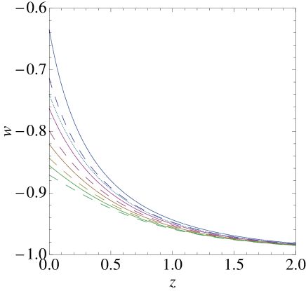
Figure 1: Plot of equation of state $w$ vs. redshift for different scalar field and tachyon models. Solid curves represent different Tachyonic models with $V(\phi)=\phi,\phi^{2},e^{\phi},\phi^{-2}$ respectively from top to bottom, Dashed curves from top to bottom represent different scalar field models with same potentials as in tachyon. Dotted curve represents PNGB model. $\Omega_{m}=0.3$.

As mentioned before, tachyon field is of interest in cosmology. There have been several investigations using this field as a dark energy candidate tachyon . In what follows, we shall repeat the above presented analysis for tachyon field.

III Thawing Tachyon Field

The tachyon field is specified by the Dirac-Born-Infeld (DBI) type of action sen

$${\mathcal{S}}=\int{-V(\phi)\sqrt{1-\partial^{\mu}\phi\partial_{\mu}\phi}}\sqrt{-g}d^{4}x.$$ (18)

In FRW background, the pressure and energy density of the tachyon field $\phi$ are given by

$$p_{\phi}=-V(\phi)\sqrt{1-\dot{\phi}^{2}}$$ (19)

$$\rho_{\phi}=\frac{V(\phi)}{\sqrt{1-\dot{\phi}^{2}}}$$ (20)

The equation of motion which follows from (18) is

$$\ddot{\phi}+3H\dot{\phi}(1-\dot{\phi}^{2})+\frac{V^{\prime}}{V}(1-\dot{\phi}^{2})=0$$ (21)

where $H$ is the Hubble parameter. The evolution equations can be cast in the following autonomous form for the convenient use

$$x^{\prime}_{t}=-(1-x_{t}^{2})(3x_{t}-\sqrt{3}\lambda_{t}y_{t})$$ (22)

$$y^{\prime}_{t}=\frac{y_{t}}{2}\left[-\sqrt{3}\lambda_{t}x_{t}y_{t}-\frac{3(1-x_{t}^{2})y_{t}^{2}}{\sqrt{1-x_{t}^{2}}}+3\right]$$ (23)

$$\lambda^{\prime}_{t}=-\sqrt{3}\lambda_{t}^{2}x_{t}y_{t}(\Gamma-\frac{3}{2})$$ (24)

with $x_{t},y_{t},\lambda_{t}$ and $\Gamma$ defined as

$$x_{t}=\dot{\phi},~{}y_{t}=\frac{\sqrt{V(\phi)}}{\sqrt{3}H},~{}\lambda_{t}=-\frac{V_{\phi}}{V^{\frac{3}{2}}},~{}\Gamma=V\frac{V_{\phi\phi}}{V_{\phi}^{2}}$$ (25)

where prime again denotes the derivative with respect to $\ln(a)$.

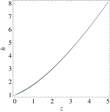
Figure 2: Plot of $h(a)=\frac{H(a)}{H_{0}}$ vs. redshift for different models as well as for $\Lambda$CDM corresponding to $\Omega_{m0}=0.3$.

We would further use the following definitions for the tachyon field as we did in case of thawing quintessence

$$\Omega_{\phi}=\frac{y^{2}}{\sqrt{1-x^{2}}},~{}~{}\gamma\equiv 1+w=\dot{\phi}^{2},$$ (26)

where $w={p_{\phi}\over{\rho_{\phi}}}$ is the equation of state for the tachyon field. One can now express the autonomous equations through them:

$$\gamma^{\prime}=-6\gamma(1-\gamma)+2\sqrt{3\gamma\Omega_{\phi}}\lambda_{t}(1-\gamma)^{\frac{5}{4}}$$ (27)

$$\Omega_{\phi}^{\prime}=3\Omega_{\phi}(1-\gamma)(1-\Omega_{\phi})$$ (28)

$$\lambda_{t}^{\prime}=-\sqrt{3\gamma\Omega_{\phi}}\lambda^{2}(1-\gamma)^{\frac{1}{4}}(\Gamma-\frac{3}{2})$$ (29)

We adopt a similar treatment to solve the above set of equation (27)-(29) as we had done in the earlier case. Infact, we even consider similar kind of potentials for tachyon fields as well, i.e, $V=\phi$, $V=\phi^{2}$,  $V=e^{\phi}$ and $V=\phi^{-2}$, characterized by $\Gamma=0,~{}\frac{1}{2},~{}1$ and $\frac{3}{2}$ respectively along with the initial conditions for $\lambda_{tinitial}$ to be $1$ and $\gamma_{initial}\sim 0$. Here also we take two solutions set for all $\Gamma$’s, with two different initial conditions of $\Omega_{\phi}$ such that at present it contributes $70\%$ and $75\%$ of the total energy share. Before discussing our result, we want to point that the system of equations (14)-(16) and (27)-(29) for scalar field and tachyon field respectively are completely different. Hence a priori one expects to have different evolutions for different potentials as well as for scalar and tachyon fields.

Once we know the solution for $\Omega_{\phi}(a)$ by solving either (14)-(16) or (27)-(29), we can easily find the behavior of the Hubble parameter which, in terms of $\Omega_{\phi}$, can be expressed as

$$h^{2}(a)=\frac{H^{2}(a)}{H_{0}^{2}}=\frac{1-\Omega_{\phi 0}}{1-\Omega_{\phi}}a^{-3},$$ (30)

where $H_{0}$ and $\Omega_{\phi 0}$ are the present day values for the Hubble parameter and the dark energy density parameter. This is the most important parameter as all the observable quantities involving background cosmology can be constructed from this. Moreover there are independent observational constraint on this parameter itself. We should mention that in this approach, one does not need to know the equation of state ($\gamma(a)=1+w(a)$) to construct the observational quantities although its effect comes through the solutions of Eqs.(14)-(16) or (27)-(29).

Figure 3: Plot of $\Delta h$(explained in the text) vs. redshift for different models. Solid curves represent different Tachyonic models with $V(\phi)=\phi,\phi^{2},e^{\phi},\phi^{-2}$ respectively from top to bottom, Dashed curves from top to bottom represent different scalar field models with same potentials as in tachyon. Dotted curve represents PNGB model. $\Omega_{m0}=0.3$. The black dots represents the value of the error bar as quoted in hubble ; ratra . We assume $h_{0}=73\pm 3kms^{-1}Mpc^{-1}$ for our purpose.

IV Results

Let us now discuss the results of our investigations. In Fig1, we plot the behavior of the equation of state $w(a)$ for different models. It shows that the equation of states of different fields with different potentials behave differently as one approaches the present day although in the past their behavior are almost identical which is not surprising as we have assumed the violation of slow-roll condition, i.e $\lambda_{initial}\sim 1$. With slow-roll condition satisfied,i.e, $\lambda_{i}<<1$, it was shown earlier that models with different potentials have the identical $w(a)$ both for scalar and tachyon fields scsen1 ; scsen2 ; amna .

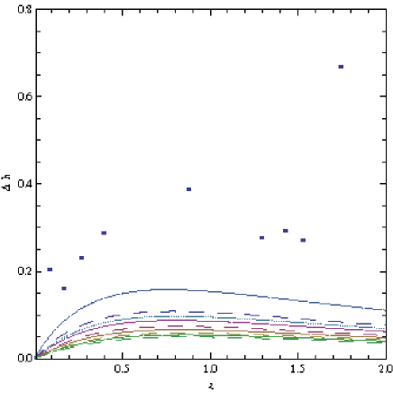
Figure 4: Plot of $\Delta h$ vs. redshift for different models same as Fig 3 but with $\Omega_{m0}=0.25$.

Next we investigated the behavior of the Hubble parameter in different cases. With different behavior for $w(a)$ as shown in Fig1, one would expect to have different behavior for Hubble parameter also. However, they are completely indistinguishable as shown in Fig 2. In this figure, we have also plotted $h(a)$ for $\Lambda$CDM. It is seen that we can not differentiate between individual models as well as these models from $\Lambda$CDM. It is interesting to note that despite having completely different behavior for equation of state, all the models have almost identical evolution for the Hubble parameter. This is crucial as all the observational quantities are constructed out of $h(a)$ at least at the level of background cosmology. In recent past, estimates of $H(z)$ were derived by Simon, Verde and Jimenez using passively evolving galaxies hubble (also see Refratra ). Keeping this in mind, we next plot the different $\Delta h=h_{field}-h_{\Lambda CDM}$ for each of our model in Fig. 3 and Fig. 4 for two different values of $\Omega_{m0}$ ($0.3$ and $0.25$) respectively. In the same figures, we have also plotted the values of the error bars $\Delta h$ (where $\Delta h={\Delta H\over{H_{0}}}+{H\Delta H_{0}\over{H_{0}^{2}}}$). We take the values of $H$ and $\Delta H$ from the the data hubble ; ratra and use the prior $H_{0}=73\pm 3kms^{-1}Mpc^{-1}$ as quoted therein. Fig.3 $\&$4 show that with $\Omega_{m0}=0.3$, one can not distinguish all the models from $\Lambda$CDM as the difference between them is much smaller than the present error bars. With smaller values of the density parameter, $\Omega_{m0}=0.25$, the difference becomes larger but the error bars still do not allow to distinguish the models from $\Lambda$CDM. The other interesting feature which one notices from both these figures, is that the difference is maximum in the redshift range from $z=0.5$ to $z=1$. Hence having more data points for higher redshifts may not be useful for the purpose to distinguish different models from $\Lambda$CDM; rather the low redshift measurements is more vital to do the needful.

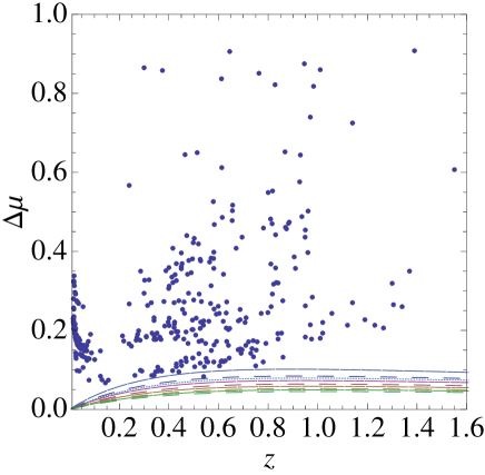
Figure 5: Plot of $\Delta\mu$(explained in the text) vs. redshift for different models. Solid curves represent different Tachyonic models with $V(\phi)=\phi,\phi^{2},e^{\phi},\phi^{-2}$ respectively from top to bottom, Dashed curves from top to bottom represent different scalar field models with same potentials as in tachyon. Dotted curve represents PNGB model. $\Omega_{m0}=0.3$. The black dots represent the value of the error bars as quoted in the Constitution data set cons .

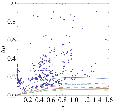
Figure 6: Plot of $\Delta\mu$ vs. redshift for different models same as Fig 5 corresponding to $\Omega_{m0}=0.25$.

Next we consider the Supernova Type-Ia observation which is one of the direct probes for late time acceleration. It measures the apparent brightness of the supernovae as observed by us which is related to the luminosity distance $d_{L}(z)$ defined as

$$d_{L}=(1+z)\int_{0}^{z}\frac{dz^{\prime}}{H(z^{\prime})}.$$ (31)

$$\begin{array}[]{|c|c|c|}\hline\cr Model&V(\phi)&D_{V\phi}-D_{V\Lambda}\\ &&for~{}\Omega_{\phi}=0.70\\ \hline\cr ThawingModel&\phi{}&-0.01464\\ \hline\cr Thawing~{}model&\phi^{2}&-0.01156\\ \hline\cr Thawing~{}model&e^{\phi}&-0.00972\\ \hline\cr Thawing~{}model&\frac{1}{\phi^{2}}&-0.00843\\ \hline\cr Scalar~{}field&M^{4}[\cos\phi+1]~{}(PNGB)&-0.01398\\ \hline\cr Tachyon&\phi&-0.01715\\ \hline\cr Tachyon&\phi^{2}&-0.01291\\ \hline\cr Tachyon&e^{\phi}&-0.01062\\ \hline\cr Tachyon&\frac{1}{\phi^{2}}&-0.00911\\ \hline\cr\end{array}$$

Table 1

With this, one constructs the distance modulus $\mu$ which is experimentally measured:

$$\mu=m-M=5log\frac{d_{L}}{Mpc}+25,$$ (32)

where $m$ and $M$ are the apparent and absolute magnitudes of the supernovae which are logarithmic measure of flux and luminosity respectively. In Fig 5 and Fig 6, we plot the difference $\Delta\mu=\mu_{\phi}-\mu_{\Lambda CDM}$ for each model together with current error bars as quoted in the latest Constitution data set cons . One can now see that with $\Omega_{m0}=0.3$ (Fig 5), the difference with $\Lambda$CDM for any model is quite small as compared to the value of the error bars. But with $\Omega_{m0}=0.25$, this difference enhances, and models like tachyon and scalar field with linear potentials as well as scalar field with PNGB potential, have significant difference with $\Lambda$CDM which is in the range of the values of the error bars. The plots also shows that the intermediate redhsift range between 0.4 and 1.0 is most sensitive to compare the models with $\Lambda$CDM and future experiments involving Type-Ia supernova should focus more in this redshift range in order to investigate the nature of dark energy.

$$\begin{array}[]{|c|c|c|}\hline\cr Model&V(\phi)&D_{V\phi}-D_{V\Lambda}\\ &&for~{}\Omega_{\phi}=0.75\\ \hline\cr ThawingModel&\phi{}&-0.02369\\ \hline\cr Thawing~{}model&\phi^{2}&-0.01667\\ \hline\cr Thawing~{}model&e^{\phi}&-0.01332\\ \hline\cr Thawing~{}model&\frac{1}{\phi^{2}}&-0.01121\\ \hline\cr Scalar~{}field&M^{4}[\cos\phi+1]~{}(PNGB)&-0.02156\\ \hline\cr Tachyon&\phi&-0.03313\\ \hline\cr Tachyon&\phi^{2}&-0.01951\\ \hline\cr Tachyon&e^{\phi}&-0.01498\\ \hline\cr Tachyon&\frac{1}{\phi^{2}}&-0.01235\\ \hline\cr\end{array}$$

Table 2

Another observational probe that has been widely used in recent times to constraint dark energy models is related to the data from the Baryon Acoustic Oscillations measurementssdss . In this case, one needs to calculate the parameter $D_{V}$ which is related to the angular diameter distance as follows

$$D_{V}(z_{BAO})=\left[\frac{z_{BAO}}{H(z_{BAO})}(\int_{0}^{z_{BAO}}\frac{dz}{H(z)})^{2}\right]^{1/3}$$ (33)

For BAO measurements we calculate the ratio $D_{V}(z=0.35)/D_{V}(z=0.20)$. As shown in percival this ratio is a relatively model independent quantity and has a value $1.812\pm 0.060$. For our case, we calculate the difference of this ratio between any scalar field model and $\Lambda$CDM model. In tables 1 $\&$ 2, we quote our result for two different values for $\Omega_{m0}:\Omega_{m}=0.3$, $\Omega_{m0}=0.25$ .

As one can see from the results quoted in these two tables, with current BAO measurements, it is hard to distinguish all the models from $\Lambda$CDM. One has to decrease the error bars at least by fifty percent for this purpose.

V Conclusion

In this paper, we have studied the general classes of thawing models with both quintessence and tachyon type scalar fields without assuming slow-roll conditions for the potentials of these fields. Our investigations show that the overall Hubble parameter has almost identical behavior for all these models and also matches with its counterpart corresponding to $\Lambda$CDM despite of the fact that the equation of state for different models behaves quite differently. Since all the observable quantities related to background evolution, are constructed out of $H(z)$, it is practically impossible to distinguish these models from $\Lambda$CDM using the current data. While analyzing the observational constraints, we used supernova and BAO data along with the information on Hubble parameter measurements. Our analysis shows that for smaller values of $\Omega_{m0}$, it is easier to distinguish amongst the various models. We find that tachyon and scalar field models with linear potential as well as scalar field model with PNGB potential are comparatively easier to distinguish from $\Lambda$CDM. It should be mentioned that little attention is paid in the literature to scalar models with linear potentials linear ; these models deserve further investigations.

An interesting outcome of our study is related to the small redshift range showing distinguished features. We find that the behavior of thawing dynamics around the redshift interval, $z=0.5$ $-1$, is most sensitive to study the deviations from $\Lambda$CDM. In our opinion, future observations should concentrate more on this particular range so as to decrease the error bars significantly.

VI Acknowledgement

A.A.S acknowledges the financial support provided by the University Grants Commission, Govt. Of India, through major research project grant (Grant No:33-28/2007(SR)). S.S acknowledges the financial support provided by University Grants Commission, Govt. Of India through the D.S.Kothari Post Doctoral Fellowship.

References

- (1) R. A. Knop et al., Ap.J. 598, 102 (2003); A. G. Riess, et al., Ap.J. 607, 665 (2004).
- (2) E. J. Copeland, M. Sami and S. Tsujikawa, Int.J.Mod.Phys.D 15, 1753 (2006); M. Sami, arXiv:0904.3445; V. Sahni and A. A. Starobinsky, Int.J.Mod.Phys.D 9, 373 (2000); T. Padmanabhan, Phys.Rep. 380, 235 (2003); E. V. Linder, astro-ph/0704.2064; J. Frieman, M. Turner and D. Huterer, arXiv:0803.0982; R. Caldwell and M. Kamionkowski, arXiv:0903.0866; A. Silvestri and M. Trodden, arXiv:0904.0024.
- (3) B. Ratra and P. J. E. Peebles, Phys.Rev.D 37, 3406 (1988); R. R. Caldwell, R. Dave and P. .J .Steinhardt, Phys.Rev.Lett. 80, 1582 (1998); A. R. Liddle and R. J. Scherrer, Phys.Rev.D 59, 023509 (1999); P. J. Steinhardt. L. .Wang and I. Zlatev, Phys.Rev.D 59, 123504 (1999)
- (4) R. Kallosh, et al., JCAP 0310, 015 (2003); P. P. Avelino, et al., Phys.Rev.D 70, 083506 (2004).
- (5) R. R. Caldwell and E. V. Linder, Phys.Rev.Lett. 95, 141301 (2007).
- (6) W. M. Vassey, et al., Ap.J. 666, 694 (2007); T. M. Davis, et al., Ap.J 666, 716 (2007).
- (7) R. J. Scherrer and A. A. Sen, Phys.Rev.D 77, 083515 (2008).
- (8) R. J. Scherrer and A. A. Sen, Phys.Rev.D 78, 067303 (2008).
- (9) A. Ali, M. Sami and A. A. Sen, arXiv:0904.1070 [astro-ph.CO].
- (10) J. A. Frieman, et al., Phys.Rev.Lett. 75, 2077 (1995).
- (11) A. Abrahamse, et al., arXiv:0712.2879.
- (12) U. Alam, V. Sahni and A.A. Staronbinsky, JCAP 0304, 002 (2003).
- (13) A. Sen, JHEP 9910, 008 (2002); A. Sen, Mod.Phys.Lett.A 17, 1797 (2002); M. R. Garousi, Nucl. Phys. B584, 284 (2000); E. A. Bergshoeff, M. de Roo, T. C. de Wit, E. Eyras, S. Panda, JHEP 0005, 009 (2000); J. Kluson, Phys.Rev. D 62, 126003 (2000); D. Kutasov and V. Niarchos, Nucl.Phys. B 666, 56 (2003).
- (14) E. J. Copeland, M. R. Garousi, M. Sami , S. Tsujikawa, Phys. Rev. D71, 043003 (2005); S. Tsujikawa and M. Sami, Phys. Lett. B603,113(2004); M. Sami, N. Savchenko and A. Toporensky, Phys. Rev. D70, 123528(2004); G. N. Felder, Lev Kofman and A. Starobinsky,JHEP 0209,026(2002); J. S. Bagla, H. K. Jassal and T. Padmanabhan, Phys. Rev. D 67, 063504 (2003); L. R. W. Abramo and F. Finelli, Phys. Lett. B 575, 165 (2003); J. M. Aguirregabiria and R. Lazkoz, Phys. Rev. D 69, 123502 (2004);
- (15) J. Simon, L. Verde, R. Jimenez, Phys.Rev.D 71, 123001 (2005).
- (16) L. Samushia and B. Ratra, Ap.J. 650, L5 (2006).
- (17) M. Hicken et al., Astrophys. J. 700 1097 (2009).
- (18) D. J. Eisensetin, et al., Ap.J. 633, 560 (2005).
- (19) W. J. Percival, et al., MNRAS 381, 1053 (2007).
- (20) J. Kratochvil, A. Linde, E. Linder and M. Shmakova, JCAP 0407, 001 (2004).