Gravitational waves in the black string braneworld

Abstract

We study gravitational waves in the black string Randall-Sundrum braneworld. We present a reasonably self-contained and complete derivation of the equations governing the evolution of gravitational perturbations in the presence of a brane localized source, and then specialize to the case of spherical radiation from a pointlike body in orbit around the black string. We solve for the resulting gravitational waveform numerically for a number of different orbital parameters.

I Introduction

The Randall-Sundrum (RS) braneworld model postulates that our universe is a 4-dimensional hypersurface embedded in 5-dimensional space Randall and Sundrum (1999a, b); Maartens (2004). One of the most remarkable features of the model is that in the 10 years since its introduction, no one has found any evidence of tension with current observations or tests of gravitational phenomena. This is despite the fact that the model incorporates a large extra dimension through which gravity is allowed to propagate. The RS model’s viability stems from the fact that it alters conventional general relativity (GR) on scales smaller than the curvature scale of the bulk spacetime $\ell$. Hence, if one chooses $\ell$ to be sufficiently small the RS model is indistinguishable from GR in many experimental or observational situations.

The principal virtue of the RS scenario is also a bit of a detriment: In order to constrain or refute the model one has to look at increasingly smaller scale phenomena. The most direct test comes from laboratory measurements of the gravitational force between two masses, which yields $\ell\lesssim 50\,\mu\text{m}$ Adelberger et al. (2003); Kapner et al. (2007). One can also examine high energy cosmological phenomena to derive observable consequences of the braneworld paradigm. The idea is that when the Hubble radius becomes smaller than the bulk curvature $H\ell\lesssim 1$, the physical scale of all interesting gravitational interactions are also smaller than $\ell$. So in these epochs, one expects the RS corrections to GR to become dominant. The spectrum of tensor perturbations in the high energy radiation RS era has been calculated and shown to the be consistent with the GR result (with minor modifications) Hiramatsu et al. (2005); Kobayashi and Tanaka (2006); Seahra (2006). On the other hand, the spectrum of scalar density perturbations is found to be enhanced over the GR expectation in the early universe, which could lead to an overproduction of primordial black holes in the RS model Cardoso et al. (2007). The behaviour of scalar perturbations during inflation has also been considered, and it was found that there were very small corrections to the power spectrum of primordial fluctuations Hiramatsu and Koyama (2006); Koyama et al. (2007).

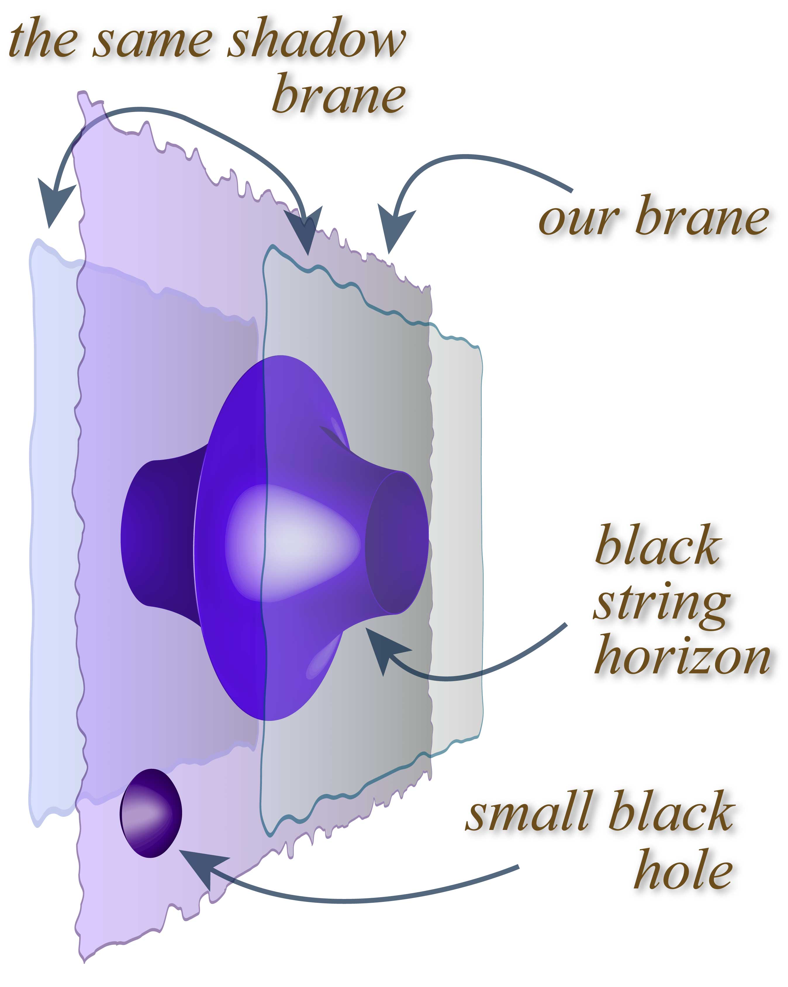
Figure 1: A schematic of the black string braneworld. The black string is a line singularity extending from our brane to a shadow brane in the bulk. There is a periodic identification such that the background geometry is symmetric about our brane. The singularity is covered by a warped horizon, and the brane separation must be large enough to be consistent with solar system tests of GR yet small enough to avoid the Gregory-Laflamme instability Gregory and Laflamme (1993); Gregory (2000); Seahra et al. (2005). In this paper, we consider the situation where the string is perturbed by a small orbiting body on one of the branes, here depicted as a small black hole.

Another possible means of constraining the RS model is with gravitational waves (GWs) with wavelengths $\lambda\lesssim\ell$. These naturally probe gravitational interactions in the regime where RS effects should be important, and can be viewed as the dynamical counterpart to the static laboratory tests of Newton’s Law mentioned above. It is useful to have a concrete model of the generation and propagation of these short-wavelength GWs in order to determine if they have sufficient amplitude to be observed by real GW detectors. To that end, we have previously considered the behaviour of gravitational perturbations around a black string braneworld (see Fig. 1) and showed that a generic feature of the signal involves a long-lived oscillatory tail composes of a discrete spectrum of modes whose wavelengths are less than $\ell$ Seahra et al. (2005). The amplitude of spherical radiation emitted by a black string being perturbed by an orbiting small body was estimated in Clarkson and Seahra (2007). This type of GW radiation is considered to be a possible source for very-high frequency GW detectors Cruise and Ingley (2006); Nishizawa et al. (2008a, b).

Our purpose in this paper is to present the details of the black string perturbative formalism utilized in the Letters Seahra et al. (2005); Clarkson and Seahra (2007). This is the subject of §II–§VII. We also describe how to numerically calculate the GWs sourced by a “point particle” orbiting the black string, and present the results of a number of simulations in §VIII.

II A generalized Randall-Sundrum two brane model

In this section, we present a generalized version of the Randall-Sundrum two brane model in a coordinate invariant formalism. Our treatment represents a generalization of the work of Shiromizu et al. (2000). We begin by outlining the geometry of the model, the action governing the dynamics, and the ensuing field equations. We then specialize to the black string braneworld model, which will be perturbed in the next section.

II.1 Geometrical framework and notation

Consider a (4+1)-dimensional manifold $(\mathcal{M},g)$, which we refer to as the ‘bulk’. One of the spatial dimensions of $\mathcal{M}$ is assumed to be compact; i.e., the 5-dimensional topology is $\mathbb{R}^{4}\times S$. We place coordinates $x^{A}$ on $\mathcal{M}$ so that the 5-dimensional line element reads:

$$ds_{5}^{2}=g_{AB}dx^{A}dx^{B}.$$ (1)

We assume that there is a scalar function $\Phi$ that uniquely maps points in $\mathcal{M}$ into the interval $I=(-d,+d]$. Here, $d$ is a constant parameter that is one of the fundamental length scales of the problem. The gradient of this mapping $\partial_{A}\Phi$ satisfies

$$\partial_{A}\Phi\,\partial^{A}\Phi>0,$$ (2)

and is tangent to the compact dimension of $\mathcal{M}$. This scalar function defines a family of timelike hypersurfaces $\Phi(x^{A})=Y$, which we denote by $\Sigma_{Y}$. The two submanifolds at the endpoints of $I$, $\Sigma_{d}$ and $\Sigma_{-d}$, are periodically identified.

Let us now place 4-dimensional coordinates $z^{\alpha}$ on each of the $\Sigma_{Y}$ hypersurfaces. These coordinates will be related to their 5-dimensional counterparts by parametric equations of the form: $x^{A}=x^{A}(z^{\alpha})$. We then define the following basis vectors

$$e^{A}_{\alpha}=\frac{\partial x^{A}}{\partial z^{\alpha}},\quad n^{A}=\frac{\partial^{A}\Phi}{\sqrt{\partial_{B}\Phi\,\partial^{B}\Phi}},$$

$$\quad n_{A}e^{A}_{\alpha}=0,\quad n^{A}n_{A}=+1.$$ (3)

The tetrad $e^{A}_{\alpha}$ is everywhere tangent to $\Sigma_{Y}$, while $n^{A}$ is everywhere normal to $\Sigma_{Y}$. The projection tensor onto the $\Sigma_{Y}$ hypersurfaces is given by

$$q_{AB}=g_{AB}-n_{A}n_{B},\quad n^{A}q_{AB}=0.$$ (4)

From this, it follows that the intrinsic line element on each of the $\Sigma_{Y}$ hypersurfaces is

$$ds^{2}_{4}=q_{\alpha\beta}dz^{\alpha}dz^{\beta},\quad q_{\alpha\beta}=e^{A}_{\alpha}e^{B}_{\beta}q_{AB}=e^{A}_{\alpha}e^{B}_{\beta}g_{AB}.$$ (5)

The object $q_{\alpha\beta}$ behaves as a tensor under 4-dimensional coordinate transformations $z^{\alpha}\rightarrow\tilde{z}^{\alpha}(z^{\beta})$ and is the induced metric on the $\Sigma_{Y}$ hypersurfaces. It has an inverse $q^{\alpha\beta}$ that can be used to define $e_{A}^{\alpha}$:

$$e_{A}^{\alpha}=g_{AB}q^{\alpha\beta}e^{B}_{\beta},\quad\delta^{\alpha}_{\beta}=q^{\alpha\gamma}q_{\gamma\beta}=e^{\alpha}_{A}e^{A}_{\beta}.$$ (6)

Generally speaking, we define the projection of any 5-tensor $T_{AB}$ onto the $\Sigma_{Y}$ hypersurfaces as

$$T_{\alpha\beta}=e^{A}_{\alpha}e^{B}_{\beta}T_{AB},$$ (7)

where the generalization to tensors of other ranks is obvious. The 4-dimensional intrinsic covariant derivative of $T_{\alpha\beta}$ is related to the 5-dimensional covariant derivative of $T_{AB}$ by

$$[\nabla_{\alpha}T_{\mu\nu}]_{q}=e^{A}_{\alpha}e^{M}_{\mu}e^{N}_{\nu}\nabla_{A}q^{B}_{M}q^{C}_{N}T_{BC},$$ (8)

where the notation $[\cdots]_{q}$ means that the quantity inside the square brackets is calculated with the $q_{\alpha\beta}$ metric.

Finally, the extrinsic curvature of each $\Sigma_{Y}$ hypersurface is:

$$K_{AB}=q^{C}_{A}\nabla_{C}n_{B}=\tfrac{1}{2}\pounds_{n}q_{AB}=K_{BA},\quad n^{A}K_{AB}=0,$$

$$K_{\alpha\beta}=e^{A}_{\alpha}e^{B}_{\beta}K_{AB}=e^{A}_{\alpha}e^{B}_{\beta}\nabla_{A}n_{B}.$$ (9)

II.2 The action and field equations

We label the hypersurfaces at $Y=y_{+}=0$ and $Y=y_{-}=+d$ as the ‘visible brane’ $\Sigma^{+}$ and ‘shadow brane’ $\Sigma^{-}$, respectively. Our observable universe is supposed to reside on the visible brane. These hypersurfaces divide the bulk into two halves: the lefthand portion $\mathcal{M}_{\text{L}}$ which has $y\in(-d,0)$, and the righthand portion which has $y\in(0,+d)$. The action for our model is:

$$S = \frac{1}{2\kappa_{5}^{2}}\int\limits_{\mathcal{M}_{\text{L}}}\left[{}^{(5)}R-2\Lambda_{5}\right]+\frac{1}{2\kappa_{5}^{2}}\int\limits_{\mathcal{M}_{\text{R}}}\left[{}^{(5)}R-2\Lambda_{5}\right]$$ (10)

$$+\sum_{\epsilon=\pm}\frac{1}{2}\int\limits_{\Sigma^{\epsilon}}\left(\mathcal{L}^{\epsilon}-2\lambda^{\epsilon}-\frac{1}{\kappa_{5}^{2}}[K]^{\epsilon}\right)$$

$$+\frac{1}{2}\int\limits_{\mathcal{M}_{\text{L}}}\mathcal{L}_{\text{L}}+\frac{1}{2}\int\limits_{\mathcal{M}_{\text{R}}}\mathcal{L}_{\text{R}}.$$

In this expression, $\kappa_{5}^{2}$ is the 5-dimensional gravity matter coupling, $\Lambda_{5}=-6k^{2}$ is the bulk cosmological constant, $\lambda^{\pm}=\pm 6k/\kappa_{5}^{2}$ are the brane tensions, and $\ell=1/k$ is the curvature length scale of the bulk. Also, $\mathcal{L}^{\pm}$ is the Lagrangian density of matter residing on $\Sigma^{\pm}$, while $\mathcal{L}_{\text{L}}$ and $\mathcal{L}_{\text{R}}$ are the Lagrangian densities of matter living in the bulk. Note that the visible brane in our model has positive tension while the shadow brane has negative tension.

The quantity $[K]^{\pm}$ is the jump in the trace of the extrinsic curvature of the $\Sigma_{Y}$ hypersurfaces across each brane. To clarify, suppose that $\partial\mathcal{M}_{\text{L}}^{\pm}$ and $\partial\mathcal{M}_{\text{R}}^{\pm}$ are the boundaries of $\mathcal{M}_{L}$ and $\mathcal{M}_{R}$ coinciding with $\Sigma^{\pm}$, respectively. Then,

$$[K]^{+} = q^{\alpha\beta}K_{\alpha\beta}\Big{|}_{\partial\mathcal{M}_{\text{R}}^{+}}-q^{\alpha\beta}K_{\alpha\beta}\Big{|}_{\partial\mathcal{M}_{\text{L}}^{+}},$$ (11a)

$${[K]^{-}} = q^{\alpha\beta}K_{\alpha\beta}\Big{|}_{\partial\mathcal{M}_{\text{L}}^{-}}-q^{\alpha\beta}K_{\alpha\beta}\Big{|}_{\partial\mathcal{M}_{\text{R}}^{-}}.$$ (11b)

We can now write down the field equations for our model. Setting the variation of $S$ with respect to the bulk metric $g^{AB}$ equal to zero yields that:

$$G_{AB}-6k^{2}g_{AB}=\kappa_{5}^{2}\left[\theta(+y)T^{\text{R}}_{AB}+\theta(-y)T^{\text{L}}_{AB}\right],$$

$$T^{\text{L,R}}_{AB}=-\frac{2}{\sqrt{-g}}\frac{\delta\left(\sqrt{-g}\mathcal{L}_{\text{L,R}}\right)}{\delta g^{AB}}.$$ (12)

Meanwhile, variation of $S$ with respect to the induced metric on each boundary yields

$$Q^{\pm}_{AB}=\left\{[K_{AB}]\pm 2kq_{AB}+\kappa_{5}^{2}(T_{AB}-\tfrac{1}{3}Tq_{AB})\right\}^{\pm}=0,\\ T_{AB}^{\pm}=e_{A}^{\alpha}e_{B}^{\beta}\left\{-\frac{2}{\sqrt{-q}}\frac{\delta\left(\sqrt{-q}\mathcal{L}\right)}{\delta q^{\alpha\beta}}\right\}^{\pm}.$$ (13)

Here, the $\{\cdots\}^{\pm}$ notation means that everything inside the curly brackets is evaluated at $\Sigma^{\pm}$. We see that (12) are the bulk field equations to be satisfied by the 5-dimensional metric $g_{AB}$, while (13) are the boundary conditions that must be enforced at the position of each brane. Of course, (13) are simply the Israel junction conditions for thin shells in general relativity. In a braneworld context, the symmetric versions of these equations first appeared in Shiromizu et al. (2000).

In what sense is our model a generalization of the RS setup? The original Randall-Sundrum model exhibited a $\mathbb{Z}_{2}$ symmetry, which implied that $\mathcal{M}_{\text{L}}$ is the mirror image of $\mathcal{M}_{\text{R}}$. Also, in the RS model the bulk was explicitly empty. However, since we allow for an asymmetric distribution of matter in the bulk, we explicitly violate the $\mathbb{Z}_{2}$ symmetry and bulk vacuum assumption.

II.3 The black string braneworld

We now introduce the black string braneworld, which is a $\mathbb{Z}_{2}$ symmetric solution of (12) and (13) with no matter sources:

$$\mathcal{L}_{\text{L}}\doteq\mathcal{L}_{\text{R}}\doteq\mathcal{L}^{\pm}\doteq 0.$$ (14)

Here, we use $\doteq$ to indicate equalities that only hold in the black string background. The bulk geometry for this solution is given by:

$$ds_{5}^{2}\doteq a^{2}(y)\left[-f(r)\,dt^{2}+\frac{1}{f(r)}\,dr^{2}+r^{2}\,d\Omega^{2}\right]+dy^{2},\\ f(r)=1-2GM/r,\quad a(y)={\rm e}^{-k|y|}.$$ (15)

Here, $M$ is the mass parameter of the black string and $G=\ell_{\text{Pl}}/M_{\text{Pl}}$ is the ordinary 4-dimensional Newton’s constant. The function $\Phi$ used to locate the branes is trivial in this background:

$$\Phi(x^{A})\doteq y,$$ (16)

which means that the $\Sigma^{\pm}$ branes are located at $y=0$ and $y=d$, respectively. The $\Sigma_{Y}\doteq\Sigma_{y}$ hypersurfaces have the geometry of Schwarzschild black holes, and there is 5-dimensional line-like curvature singularity at $r=0$:

$$R^{ABCD}R_{ABCD}\doteq\frac{48G^{2}M^{2}e^{4k|y|}}{r^{6}}+40k^{2}.$$ (17)

Note that the other singularities at $y=\pm\infty$ are excised from our model by the restriction $y\doteq Y\in(-d,d]$, so we will not consider them further.

Finally, note that the normal and extrinsic curvature associated with the $\Sigma_{Y}$ hypersurfaces satisfy the following convenient properties:

$$n_{A}\doteq\partial_{A}y,\quad n^{A}\nabla_{A}n^{B}\doteq 0,\quad K_{AB}\doteq-kq_{AB}.$$ (18)

These expressions are used liberally below to simplify formulae evaluated in the black string background.

III Linear perturbations

We now turn attention to perturbations of the black sting braneworld. Our treatment will be a reformulated and generalized version of the original Randall-Sundrum work Randall and Sundrum (1999a, b) and the seminal contribution of Garriga and Tanaka (2000).

III.1 Perturbative variables

We are ultimately interested in the behaviour of gravitational waves in this model, which are described by fluctuations of the bulk metric:

$$g_{AB}\rightarrow g_{AB}+h_{AB},$$ (19)

where $h_{AB}$ is understood to be a ‘small’ quantity. The projection of $h_{AB}$ onto the visible brane is the observable that can potentially be measured in gravitational wave detectors. But it is not sufficient to consider fluctuations in the bulk metric alone — to get a complete picture, we must also allow for the perturbation of the matter content of the model as well as the positions of the branes.

Obviously, matter perturbations are simply described by the $T_{AB}^{\text{L}}$, $T_{AB}^{\text{R}}$, and $T_{AB}^{\pm}$ stress-energy tensors, which are considered to be small quantities of the same order as $h_{AB}$. On the other hand, we describe fluctuations in the brane positions via a perturbation of the scalar function $\Phi$:

$$\Phi(x^{A})\rightarrow y+\xi(x^{A}).$$ (20)

Here, $\xi$ is a small spacetime scalar. Recall that the position of each brane is implicitly defined by $\Phi(x^{A})=y_{\pm}$. Hence, the brane locations after perturbation are given by the solution of the following for $y$:

$$y+\xi\Big{|}_{y=y_{\pm}}+(y-y_{\pm})\partial_{y}\xi\Big{|}_{y=y_{\pm}}+\cdots=y_{\pm}.$$ (21)

However, note that $y-y_{\pm}$ is of the same order as $\xi$, so at the linear level the new brane positions are simply given by

$$y=y_{\pm}-\xi\Big{|}_{y=y_{\pm}}.$$ (22)

Hence, the perturbed brane positions are given by the brane bending scalars:

$$\xi^{\pm}=\xi\Big{|}_{y=y_{\pm}},\quad n^{A}\partial_{A}\xi^{\pm}=0.$$ (23)

Note that because $\xi^{+}$ and $\xi^{-}$ are explicitly evaluated at the brane positions, they are essentially 4-dimensional scalars that exhibit no dependence on the extra dimension.

Having now delineated a set of variables that parameterize the fluctuations of the black string braneworld, we now need to determine their equations of motion.

III.2 Linearizing the bulk field equations

First, we linearize the bulk field equations (12) about the black string solution. Notice that (12) only depends on the bulk metric and the bulk matter distribution. Hence, the linearized field equations will only involve $h_{AB}$, $T_{AB}^{\text{L}}$ and $T_{AB}^{\text{R}}$. The actual derivation of the equation proceeds in the same manner as in 4-dimensions, and we just quote the result:

$$\nabla^{C}\nabla_{C}h_{AB}-\nabla^{C}\nabla_{A}h_{BC}-\nabla^{C}\nabla_{B}h_{AC}\\ +\nabla_{A}\nabla_{B}h^{C}{}_{C}-8k^{2}h_{AB}=-2\kappa_{5}^{2}\Sigma_{AB}^{\text{bulk}},$$ (24)

where

$$\Sigma_{AB}^{\text{bulk}}=\Theta(+y)(T^{\text{R}}_{AB}-\tfrac{1}{3}T^{\text{R}}g_{AB})\\ +\Theta(-y)(T^{\text{L}}_{AB}-\tfrac{1}{3}T^{\text{L}}g_{AB}).$$ (25)

The wave equation (24) is valid for arbitrary choices of gauge and generic matter sources. If we specialize to the Randall-Sundrum gauge

$$\nabla^{A}h_{AB}=0,\quad h^{A}{}_{A}=0,\quad h_{AB}=e_{A}^{\alpha}e_{B}^{\beta}h_{\alpha\beta},$$ (26)

eq. (24) reduces to

$$\hat{\Delta}_{AB}{}^{CD}h_{CD}+(GMa)^{2}(\pounds_{n}^{2}-4k^{2})h_{AB}\\ =-2(GMa)^{2}\kappa_{5}^{2}\Sigma_{AB}^{\text{bulk}},$$ (27)

where we have defined the operator

$$\hat{\Delta}_{AB} {}^{CD}=(GMa)^{2}[q^{MN}\nabla_{M}q^{P}_{N}q^{C}_{A}q^{D}_{B}\nabla_{P}+2{}^{(4)}\!R_{A}{}^{C}{}_{B}{}^{D}]$$

$$= \,(GMa)^{2}e_{A}^{\alpha}e_{B}^{\beta}\Big{[}\delta_{\alpha}^{\gamma}\delta_{\beta}^{\delta}\nabla^{\rho}\nabla_{\rho}+2{R}_{\alpha}\!{}^{\gamma}\!{}_{\beta}\!{}^{\delta}\Big{]}_{q}e^{C}_{\gamma}e^{D}_{\delta}$$

$$= \,(GM)^{2}e_{A}^{\alpha}e_{B}^{\beta}\Big{[}\delta_{\alpha}^{\gamma}\delta_{\beta}^{\delta}\nabla^{\rho}\nabla_{\rho}+2{R}_{\alpha}\!{}^{\gamma}\!{}_{\beta}\!{}^{\delta}\Big{]}_{g}e^{C}_{\gamma}e^{D}_{\delta}.$$ (28)

Here, ${}^{(4)}\!R_{ACBD}$ is the Riemann tensor on $\Sigma_{y}$, which can be related to the 5-dimensional curvature tensor via the Gauss equation

$${}^{(4)}\!R_{MNPQ}=q^{A}_{M}q^{B}_{N}q^{C}_{P}q^{D}_{Q}R_{ABCD}+2K_{M[P}K_{Q]N}.$$ (29)

On the second line of (28) the 4-tensor inside the square brackets is calculated using $q_{\alpha\beta}$. We can re-express this object in terms of the ordinary Schwarzschild metric $g_{\alpha\beta}$, which is conformally related to $q_{\alpha\beta}$ via the warp factor:

$$q_{\alpha\beta}=a^{2}g_{\alpha\beta},$$ (30a)

$$g_{\alpha\beta}dz^{\alpha}dz^{\beta}=-f\,dt^{2}+f^{-1}\,dr^{2}+r^{2}d\Omega^{2}.$$ (30b)

The quantity in square brackets on the third line of (28) is calculated from $g_{\alpha\beta}$. One can easily confirm that $\hat{\Delta}_{AB}{}^{CD}$ is ‘$y$-independent’ in the sense that it commutes with the Lie derivative in the $n^{A}$ direction:

$$[{}^{(4)}\!\hat{\Delta}_{AB}{}^{CD},\pounds_{n}]=0.$$ (31)

In addition, the $(GM)^{2}$ prefactor makes $\hat{\Delta}_{AB}{}^{CD}$ dimensionless.

Notice that the lefthand side of (27) is both traceless and manifestly orthogonal to $n^{A}$, which implies the following constraints on the bulk matter:

$$\Sigma_{AB}^{\text{bulk}}=e^{\alpha}_{A}e^{\beta}_{B}\Sigma_{\alpha\beta}^{\text{bulk}},\quad q^{\alpha\beta}\Sigma_{\alpha\beta}^{\text{bulk}}=0.$$ (32)

In other words, our gauge choice is inconsistent with bulk matter that violates these conditions. If we wish to consider more general bulk matter, we cannot use the Randall-Sundrum gauge.

III.3 Linearizing the junction conditions

Next, we consider the perturbation of the junction conditions (13). These can be re-written as

$$Q_{AB}^{\pm}=\Big{\{}[\tfrac{1}{2}\nabla_{(A}n_{B)}-n_{(A|}n^{C}\nabla_{C}n_{|B)}]\\ \pm kq_{AB}+\kappa_{5}^{2}\left(T_{AB}-\tfrac{1}{3}Tq_{AB}\right)\Big{\}}^{\pm}=0.$$ (33)

We require that $Q_{AB}^{\pm}$ vanish before and after perturbation, so we need to enforce that the first order variation $\delta Q_{AB}^{\pm}$ is equal to zero.

In order to calculate this variation, we can regard the tensors $Q_{AB}^{\pm}$ as functionals the brane positions (as defined by $\Phi$), the brane normals $n_{A}$, the bulk metric, and the brane matter:

$$Q_{AB}^{\pm}=Q_{AB}^{\pm}(\Phi,n_{M},g_{MN},T^{\pm}_{MN}),$$ (34)

from which it follows that

$$\delta Q_{AB}^{\pm}=\left\{\frac{\delta Q_{AB}}{\delta\Phi}\delta\Phi+\frac{\delta Q_{AB}}{\delta n_{C}}\delta n_{C}\right.\\ \left.+\frac{\delta Q_{AB}}{\delta g_{CD}}\delta g_{CD}+\frac{\delta Q_{AB}}{\delta T_{CD}}\delta T_{CD}\right\}_{0}^{\pm}.$$ (35)

The $\{\cdots\}^{\pm}_{0}$ notation is meant to remind us that after we have calculated the variational derivatives, we must evaluate the expression in the background geometry at the unperturbed positions of the brane.

We now consider each term in (35). For simplicity, we temporarily focus on the positive tension visible brane and drop the + superscript. The first term represents the variation of $Q_{AB}^{\pm}$ with brane position, which is covariantly given by the Lie derivative in the normal direction:

$$\left\{\frac{\delta Q_{AB}}{\delta\Phi}\delta\Phi\right\}_{0}=\left\{-\xi\pounds_{n}Q_{AB}\right\}_{0}.$$ (36)

But the Lie derivative of $Q_{AB}$ vanishes identically in the background geometry, so this term is equal to zero.

The second term in (35) represents the variation of $Q_{AB}$ with respect to the normal vector. Making note of the definition (3) of $n^{A}$ in terms of $\Phi$, as well as $\delta\Phi=\xi$ and $n^{A}\nabla_{A}\xi=0$, we arrive at

$$\delta n_{A}=\nabla_{A}\xi,\quad n^{A}\delta n_{A}=0.$$ (37)

Notice that since the normal itself must be continuous across the brane, we have $[\delta n_{A}]=0$. After some algebra, we find that the variation of the junction conditions with respect to the brane normal is non-zero and given by

$$\left\{\frac{\delta Q_{AB}}{\delta n_{C}}\delta n_{C}\right\}_{0}=2q^{C}_{A}q^{D}_{B}\nabla_{C}\nabla_{D}\xi.$$ (38)

The third term in (35) is the variation with the bulk metric itself $\delta g_{AB}=h_{AB}$. Calculating this is straightforward, and the result is:

$$\left\{\frac{\delta Q_{AB}}{\delta g_{CD}}\delta g_{CD}\right\}_{0}=\tfrac{1}{2}[\pounds_{n}h_{AB}]+2kh_{AB}.$$ (39)

The last variation we must consider is with respect to the brane matter fields, which is trivial:

$$\left\{\frac{\delta Q_{AB}}{\delta T_{CD}}\delta T_{CD}\right\}_{0}=\kappa_{5}^{2}\left(T_{AB}-\tfrac{1}{3}Tq_{AB}\right).$$ (40)

So, we have the final result that

$$\delta Q_{AB}^{\pm}=\left\{2q^{C}_{A}q^{D}_{B}\nabla_{C}\nabla_{D}\xi+\tfrac{1}{2}[\pounds_{n}h_{AB}]\right.\\ \left.\pm 2kh_{AB}+\kappa_{5}^{2}\left(T_{AB}-\tfrac{1}{3}Tq_{AB}\right)\right\}_{0}^{\pm}=0.$$ (41)

If we take the trace of $\delta Q_{AB}^{\pm}=0$, we obtain

$$q^{AB}\nabla_{A}\nabla_{B}\xi^{\pm}=\tfrac{1}{6}\kappa_{5}^{2}T^{\pm}.$$ (42)

These are the equations of motion for the brane bending degrees of freedom in our model, which are seen to be directly sourced by the matter fields on each brane.

III.4 Converting the boundary conditions into distributional sources

We can incorporate the boundary conditions $\delta Q_{AB}^{\pm}=0$ directly into the $h_{AB}$ equation of motion as delta-function sources. This is possible because the jump in the normal derivative of $h_{AB}$ appears explicitly in the perturbed junction conditions. This procedure gives

$$\hat{\Delta}_{AB}{}^{CD}h_{CD}-\hat{\mu}^{2}h_{AB}\\ =-2(GMa)^{2}\kappa_{5}^{2}\left[\Sigma_{AB}^{\text{bulk}}+\sum_{\epsilon=\pm}\delta(y-y_{\epsilon})\Sigma_{AB}^{\epsilon}\right].$$ (43)

Here, we have defined

$$\hat{\mu}^{2}=-(GMa)^{2}\left[\pounds_{n}^{2}+\frac{2\kappa_{5}^{2}}{3}\sum_{\epsilon=\pm}\lambda^{\epsilon}\delta(y-y_{\epsilon})-4k^{2}\right],$$

$$\Sigma_{AB}^{\pm}=\left(T^{\pm}_{AB}-\tfrac{1}{3}T^{\pm}q_{AB}\right)+\frac{2}{\kappa_{5}^{2}}q^{C}_{A}q^{D}_{B}\nabla_{C}\nabla_{D}\xi^{\pm}.$$ (44)

If we integrate the wave equation (43) over a small region traversing either brane, we recover the boundary conditions (41).

Together with the gauge conditions,

$$n^{A}h_{AB}=q^{AC}\nabla_{A}h_{CB}=0=q^{AB}h_{AB},$$ (45)

(42) and (43) are the equations governing the perturbations of our model.

IV Kaluza-Klein mode functions

IV.1 Separation of variables

As mentioned above, we have that

$$[\hat{\Delta}_{AB}{}^{CD},\pounds_{n}]h_{CD}=0;$$ (46)

i.e., $\hat{\Delta}_{AB}{}^{CD}$ is independent of $y$ when evaluated in the $(t,r,\theta,\phi,y)$ coordinates. This suggests that we seek a solution for $h_{AB}$ of the form

$$h_{AB}=Z\tilde{h}_{AB},\quad\hat{\mu}^{2}Z=\mu^{2}Z,$$ (47)

where,

$$0=\pounds_{n}\tilde{h}_{AB}\text{ and }0=q^{A}_{B}\nabla_{A}Z;$$ (48)

that is, $Z$ is an eigenfunction of $\hat{\mu}^{2}$ with eigenvalue $\mu^{2}$. The existence of the delta functions in the $\hat{\mu}^{2}$ operator means that we need to treat the even and odd parity solutions of this eigenvalue problem separately.

IV.2 Even parity eigenfunctions

If $Z(-y)=Z(y)$, we see that $Z$ satisfies the following equations in the interval $y\in[0,d]$:

$$\begin{split}m^{2}Z(y)&=-a^{2}(y)(\partial_{y}^{2}-4k^{2})Z(y),\\ 0&=[(\partial_{y}+2k)Z(y)]_{\pm},\\ \mu&=GMm.\end{split}$$ (49)

There is a discrete spectrum of solutions to this eigenvalue problem that are labeled by the positive integers $n=1,2,3\ldots$:

$$Z_{n}(y)=\alpha_{n}^{-1}[Y_{1}(m_{n}\ell)J_{2}(m_{n}\ell e^{k|y|})\\ -J_{1}(m_{n}\ell)Y_{2}(m_{n}\ell e^{k|y|})],$$ (50)

where $\alpha_{n}$ is a constant, and $m_{n}=\mu_{n}/GM$ is the $n^{\text{th}}$ solution of

$$Y_{1}(m_{n}\ell)J_{1}(m_{n}\ell e^{kd})=J_{1}(m_{n}\ell)Y_{1}(m_{n}\ell e^{kd}).$$ (51)

There is also a solution corresponding to $m_{0}=\mu_{0}=0$, which is known as the zero-mode:

$$Z_{0}(y)=\alpha_{0}^{-1}e^{-2k|y|},\quad\alpha_{0}=\sqrt{\ell}(1-e^{-2kd})^{1/2}.$$ (52)

Hence, there exists a discrete set of solutions for bulk metric perturbations of the form $h_{AB}^{(n)}=Z_{n}(y)\tilde{h}_{AB}^{(n)}(z^{\alpha})$. When $n>0$ these are called the Kaluza-Klein (KK) modes of the modes, and the mass of any given mode is given by the $m_{n}$ eigenvalue. The $\alpha_{n}$ constants are determined from demanding that $\{Z_{n}\}$ forms an orthonormal set

$$\delta_{mn}=\int_{-d}^{d}dy\,a^{-2}(y)Z_{m}(y)Z_{n}(y).$$ (53)

These basis functions then satisfy:

$$\delta(y-y_{\pm})=\sum_{n=0}^{\infty}a^{-2}Z_{n}(y)Z_{n}(y_{\pm}).$$ (54)

This identity is crucial to the model — inspection of (43) reveals that the brane stress energy tensors appearing on the righthand side are multiplied by one of $\delta(y-y_{\pm})$. Hence, brane matter only couples to the even parity eigenmodes of $\hat{\mu}^{2}$.

Case 1: light modes

It is useful to have simple approximate forms of the Kaluza-Klein masses and normalization constants. These are straightforward to derive for modes that are ‘light’ compared to mass scale set by the AdS₅ length parameter:

$$m_{n}\ell\ll 1.$$ (55)

Let us define a set of dimensionless numbers $x_{n}$ by:

$$x_{n}=m_{n}\ell e^{kd}.$$ (56)

Then for the light modes, we find that $x_{n}$ is the $n^{\text{th}}$ zero of the first-order Bessel function:

$$J_{1}(x_{n})=0.$$ (57)

Also for light modes, the normalization constants reduce to

$$\alpha_{n}\approx 2\sqrt{\ell}\,e^{2kd}|J_{0}(x_{n})|/\pi x_{n},\quad n>0.$$ (58)

Actually, it is more helpful to know the value of the KK mode functions at the position of each brane. We can parameterize these as

$$Z_{n}(y_{\pm})=\sqrt{k}e^{-kd}z_{n}^{\pm},\quad n>0.$$ (59)

For the light Kaluza-Klein modes, the dimensionless $z_{n}^{\pm}$ are given by

$$z_{n}^{\pm}\approx\left\{\genfrac{}{}{0.0pt}{0}{|J_{0}(x_{n})|^{-1}}{e^{in\pi}}\right\}.$$ (60)

Case 2: heavy modes

At the other end of the spectrum, we have the heavy Kaluza-Klein modes

$$m_{n}\ell\gg 1.$$ (61)

Under this assumption, we find

$$x_{n} \approx \frac{n\pi}{1-e^{-kd}},$$ (62a)

$$Z_{n}(y) \approx \sqrt{\frac{ke^{-k|y|}}{e^{kd}-1}}\cos\left[n\pi\frac{e^{k|y|}-1}{e^{kd}-1}\right],$$ (62b)

$$z_{n}^{\pm} \approx \frac{1}{\sqrt{1-e^{-kd}}}\left\{\genfrac{}{}{0.0pt}{0}{e^{kd/2}}{e^{in\pi}}\right\}.$$ (62c)

(Strictly speaking, an asymptotic analysis leads to formulae with $n$ replaced by another integer $n^{\prime}$ on the righthand sides of Eqns. (62). However, we note that for even parity modes, $n$ counts the number of zeroes of $Z_{n}(y)$ in the interval $y\in(0,d)$, which allows us to deduce that $n^{\prime}=n$.) Unlike the analogous quantities for the light modes, $z_{n}^{\pm}$ shows an explicit dependence on the dimensionless brane separation $d/\ell$.

IV.3 Odd parity eigenfunctions

As mentioned above, brane matter only couples to Kaluza-Klein modes with even parity. But a complete perturbative description must include the odd parity modes as well; for example, if we have matter in the bulk distributed asymmetrically with respect to $y=0$ (i.e. $T_{AB}^{\text{L}}\neq T_{AB}^{\text{R}}$) modes of either parity will be excited. Hence, for the sake of completeness, we list a few properties of the odd parity Kaluza-Klein modes here.

Assuming $Z(-y)=-Z(y)$, we have:

$$\begin{split}m^{2}Z(y)&=-a^{2}(y)(\partial_{y}^{2}-4k^{2})Z(y),\\ 0&=Z(y_{+})=Z(y_{-}).\end{split}$$ (63)

Again, we have a discrete spectrum of solutions, this time labeled by half integers:

$$Z_{n+\frac{1}{2}}(y)=\alpha_{n+\frac{1}{2}}^{-1}[Y_{2}(m_{n+\frac{1}{2}}\ell)J_{2}(m_{n+\frac{1}{2}}\ell e^{k|y|})\\ -J_{2}(m_{n+\frac{1}{2}}\ell)Y_{2}(m_{n+\frac{1}{2}}\ell e^{k|y|})].$$ (64)

The mass eigenvalues are now the solutions of

$$Y_{2}(m_{n+\frac{1}{2}}\ell)J_{2}(m_{n+\frac{1}{2}}\ell e^{kd})=\\ J_{2}(m_{n+\frac{1}{2}}\ell)Y_{2}(m_{n+\frac{1}{2}}\ell e^{kd}).$$ (65)

Proceeding as before, we define

$$x_{n+\frac{1}{2}}=m_{n+\frac{1}{2}}\ell e^{kd}.$$ (66)

For light modes with $m_{n+\frac{1}{2}}\ell\ll 1$, $x_{n+\frac{1}{2}}$ is the $n^{\text{th}}$ zero of the second-order Bessel function:

$$J_{2}(x_{n+\frac{1}{2}})=0.$$ (67)

Taken together, (57) and (67) imply the following for the light modes:

$$m_{1}<m_{3/2}<m_{2}<m_{5/2}<\cdots;$$ (68)

i.e., the first odd mode is heavier than the first even mode, etc.

Finally, we note that since the odd modes vanish at the background position of the visible brane, it is impossible for us to observe them directly within the context of linear theory. This can change at second order, since brane bending can allow us to directly sample regions of the bulk where $Z_{n+\frac{1}{2}}\neq 0$. However, this phenomenon is clearly beyond the scope of this paper.

IV.4 Stability criterion

Finally, as discussed in detail elsewhere Seahra et al. (2005), the black string braneworld will be perturbatively stable if the smallest KK mass satisfies

$$\mu_{1}=GMm_{1}>\mu_{c}\approx 0.4301.$$ (69)

Under the approximation that the first mode is light ($x_{1}e^{-kd}\ll 1$) and using $G=\ell_{\text{Pl}}/M_{\text{Pl}}$, this gives a restriction on the black string mass

$$\frac{M}{M_{\text{Pl}}}\gtrsim\frac{\ell}{\ell_{\text{Pl}}}\frac{\mu_{c}}{x_{1}}e^{kd},$$ (70)

or equivalently,

$$\frac{M}{M_{\odot}}\gtrsim 8\times 10^{-9}\left(\frac{\ell}{\text{0.1 mm}}\right)e^{d/\ell}.$$ (71)

If we take $\ell=$ 0.1 mm, then we see that all solar mass black holes will in actuality be stable black strings provided that $d/\ell\lesssim 19$.

V Recovering 4-dimensional gravity

Let us now describe the limit in which we recover general relativity. (Garriga and Tanaka (2000) first considered this problem in Minkowski space, but the approach employed here is somewhat different.) We assume there are no matter perturbations in the bulk and on the hidden brane; hence, we may consistently neglect the odd parity Kaluza-Klein modes. By virtue of the brane bending equation of motion (42), we can consistently set $\xi^{-}=0$. Furthermore, (54) can be used to replace the delta function in front of $\Sigma_{AB}^{+}$ in equation (43). We obtain,

$$\hat{\Delta}_{AB}{}^{CD}h_{CD}-\hat{\mu}^{2}h_{AB}\\ =-2(GM)^{2}\kappa_{5}^{2}\Sigma_{AB}^{+}\sum_{n=0}^{\infty}Z_{n}(y_{+})Z_{n}(y).$$ (72)

We now note that for $e^{-kd}\ll 1$,

$$Z_{0}(y_{+})=\sqrt{k}(1-e^{-2kd})^{-1/2}\gg Z_{n}(y_{+}),\quad n>0.$$ (73)

That is, the $n>0$ terms in the sum are much smaller than the $0^{\text{th}}$ order contribution. This motivates an approximation where the $n>0$ terms on the righthand side of (72) are neglected, which is the so-called ‘zero-mode truncation’.

When this approximation is enforced, we find that $h_{AB}$ must be proportional to $Z_{0}(y)$; i.e., there is no contribution to $h_{AB}$ from any of the KK modes. Hence, we have $\hat{\mu}^{2}h_{AB}=0$. The resulting expression has trivial $y$ dependence, so we can freely set $y=y_{+}$ to obtain the equation of motion for $h_{AB}$ at the unperturbed position of the visible brane:

$$\hat{\Delta}_{AB}{}^{CD}h^{+}_{CD}=-2(GM)^{2}\kappa_{5}^{2}\Sigma_{AB}^{+}Z^{2}_{0}(y_{+})$$ (74)

But we are not really interested in $h_{AB}^{+}$, the physically relevant quantity is the perturbation of the induced metric on the perturbed brane, which is defined as the variation of

$$q_{AB}^{+}=[g_{AB}-n_{A}n_{B}]^{+}.$$ (75)

We calculate $\delta q^{+}_{AB}$ in the same way as we calculated $\delta Q_{AB}^{\pm}$ above (except for the fact that $q_{AB}$ shows no explicit dependence on $T_{AB}^{+}$):

$$\delta q_{AB}^{+}=\left\{\frac{\delta q_{AB}}{\delta\Phi}\delta\Phi+\frac{\delta q_{AB}}{\delta n_{C}}\delta n_{C}+\frac{\delta q_{AB}}{\delta g_{CD}}\delta g_{CD}\right\}_{0}^{+}.$$ (76)

These variations are straightforward, and we obtain:

$$\delta q_{AB}^{+}\equiv\bar{h}_{AB}^{+}=h^{+}_{AB}+2k\xi^{+}q_{AB}^{+}\\ -(n_{A}\nabla_{B}+n_{B}\nabla_{A})\xi^{+},$$ (77)

where all quantities on the right are evaluated in the background and at the unperturbed position of the brane. Note that $\bar{h}_{AB}n^{A}\neq 0$, which reflects the fact that $n_{A}$ is no longer the normal to the brane after perturbation.

We now define the 4-tensors

$$\bar{h}_{\alpha\beta}^{+}=e^{A}_{\alpha}e^{B}_{\beta}\bar{h}_{AB}^{+},\quad T^{+}_{\alpha\beta}=e^{A}_{\alpha}e^{B}_{\beta}T^{+}_{AB}.$$ (78)

Here, $\bar{h}_{\alpha\beta}^{+}$ is the actual metric perturbation on the visible brane. Note that this perturbation is neither transverse or tracefree:

$$\nabla^{\gamma}\bar{h}^{+}_{\gamma\alpha}=2k\nabla_{\alpha}\xi^{+},\quad g^{\alpha\beta}\bar{h}^{+}_{\alpha\beta}=8k\xi^{+}.$$ (79)

We can now re-express the equation of motion (74) in terms of $\bar{h}^{+}_{\alpha\beta}$ instead of $h_{AB}^{+}$ using (77). Dropping the $+$ superscripts, we obtain

$$\nabla^{\gamma}\nabla_{\gamma}\bar{h}_{\alpha\beta}+\nabla_{\alpha}\nabla_{\beta}\bar{h}^{\gamma}\!{}_{\gamma}-\nabla^{\gamma}\nabla_{\alpha}\bar{h}_{\beta\gamma}-\nabla^{\gamma}\nabla_{\beta}\bar{h}_{\alpha\gamma}=\\ -2Z_{+}^{2}\kappa_{5}^{2}\left[T_{\alpha\beta}-\frac{1}{3}\left(1+\frac{k}{2Z^{2}_{+}}\right)T^{\gamma}\!{}_{\gamma}g_{\alpha\beta}\right]\\ +(6k-4Z_{+}^{2})\nabla_{\alpha}\nabla_{\beta}\xi,$$ (80)

where we have defined

$$Z_{+}^{2}=Z^{2}_{0}(y_{+})=k(1-e^{-2kd})^{-1}.$$ (81)

In obtaining this expression, we have made use of the $\xi$ equation of motion:

$$g^{\alpha\beta}\nabla_{\alpha}\nabla_{\beta}\xi=\tfrac{1}{6}\kappa_{5}^{2}g^{\alpha\beta}T_{\alpha\beta}.$$ (82)

Note that we still have the freedom to make a gauge transformation on the brane that involves an arbitrary 4-dimensional coordinate transformation generated by $\eta_{\alpha}$:

$$\bar{h}_{\alpha\beta}\rightarrow\bar{h}_{\alpha\beta}+\nabla_{\alpha}\eta_{\beta}+\nabla_{\beta}\eta_{\alpha}.$$ (83)

We can use this gauge freedom to impose the condition

$$\nabla_{\beta}\bar{h}^{\beta}\!{}_{\alpha}-\tfrac{1}{2}\nabla_{\alpha}\bar{h}^{\beta}\!{}_{\beta}=(2Z_{+}^{2}-3k)\nabla_{\alpha}\xi.$$ (84)

Then, the equation of motion for 4-metric fluctuations reads

$$\nabla^{\gamma}\nabla_{\gamma}\bar{h}_{\alpha\beta}+2R_{\alpha}\!{}^{\gamma}\!{}_{\beta}\!{}^{\delta}\bar{h}_{\gamma\delta}=\\ -16\pi G\left[T_{\alpha\beta}-\left(\frac{1+\omega_{\text{\tiny BD}}}{3+2\omega_{\text{\tiny BD}}}\right)T^{\gamma}\!{}_{\gamma}g_{\alpha\beta}\right],$$ (85)

where we have identified

$$\omega_{\text{\tiny BD}}=\frac{3}{2}(e^{2d/\ell}-1),\quad G=\frac{\kappa_{5}^{2}}{8\pi\ell(1-e^{-2d/\ell})}.$$ (86)

We see that (85) matches the equation governing gravitational waves in a Brans-Dicke theory with parameter $\omega_{\text{\tiny BD}}$. Hence in the zero-mode truncation, the perturbations of the black string braneworld are indistinguishable from a 4-dimensional scalar tensor theory.

Note that (85) must hold everywhere in our model, so we can consider the situation where our solar system is the perturbative brane matter located somewhere in the extreme far-field region of the black string. The forces between the various celestial bodies will be governed by (85) in the $R_{\alpha\beta\gamma\delta}\approx 0$ limit. In this scenario, solar system tests of general relativity Will (2005) place bounds on the Brans-Dicke parameter, and hence $d/\ell$:

$$\omega_{\text{\tiny BD}}\gtrsim 4\times 10^{4}\quad\Rightarrow\quad d/\ell\gtrsim 5.$$ (87)

This lower bound on the dimensionless brane separation will be an important factor in the discussion below.

VI Spherical waves on the brane

In this section, we specialize to the situation where there is perturbative matter located on one of the branes and no other sources. Unlike Sec. V, our interest here is to predict deviations from general relativity, so we will not use the zero-mode truncation. Principally for reasons of simplicity, we will focus on spherically symmetric radiation, which is a channel unavailable in the standard 4-dimensional setup.

VI.1 Mode decomposition

To begin, we make the assumptions

$$\Sigma^{\text{bulk}}_{AB}=0,\text{ and }\Sigma_{AB}^{+}=0\text{ or }\Sigma_{AB}^{-}=0;$$ (88)

i.e., we set the matter perturbation in the bulk and one of the branes equal to zero. Note that due to the linearity of the problem we can always add up solutions corresponding to different types of sources; hence, if we had a physical situation with many different types of matter, it would be acceptable to solve for the radiation pattern induced by each source separately and then sum the results.

We decompose $h_{AB}$ as

$$h_{AB}=\frac{\kappa_{5}^{2}(GM)^{2}}{\mathcal{C}}e_{A}^{\alpha}e_{B}^{\beta}\sum_{n=0}^{\infty}Z_{n}(y)Z_{n}(y_{\pm})h_{\alpha\beta}^{(n)}.$$ (89)

Here, $\mathcal{C}$ is a normalization constant (to be specified later) with dimensions of $(\text{mass})^{-4}$, and the expansion coefficients $h_{\alpha\beta}^{(n)}$ are dimensionless. We define a dimensionless brane stress-energy tensors and brane bending scalars by

$$\Theta^{\pm}_{\alpha\beta}=\mathcal{C}e^{A}_{\alpha}e^{B}_{\beta}T^{\pm}_{AB},\quad\tilde{\xi}^{\pm}=\frac{\mathcal{C}\xi^{\pm}}{(GM)^{2}\kappa_{5}^{2}}.$$ (90)

Omitting the $\pm$ superscripts, we find that the equation of motion for $h_{\alpha\beta}^{(n)}$ is

$$(GM)^{2}\left[\nabla^{\gamma}\nabla_{\gamma}h^{(n)}_{\alpha\beta}+2R_{\alpha}\!{}^{\gamma}\!{}_{\beta}\!{}^{\delta}h^{(n)}_{\gamma\delta}\right]-\mu_{n}^{2}h^{(n)}_{\alpha\beta}=\\ -2\left(\Theta_{\alpha\beta}-\tfrac{1}{3}\Theta g_{\alpha\beta}\right)-4(GM)^{2}\nabla_{\alpha}\nabla_{\beta}\tilde{\xi},$$ (91)

while the equation of motion for $\tilde{\xi}$ is

$$\nabla^{\alpha}\nabla_{\alpha}\tilde{\xi}=\tfrac{1}{6}\Theta.$$ (92)

We also have the conditions

$$\nabla^{\alpha}h_{\alpha\beta}^{(n)}=\nabla^{\alpha}\Theta_{\alpha\beta}=0=g^{\alpha\beta}h_{\alpha\beta}^{(n)}.$$ (93)

Note that in all of these equations, all 4-dimensional quantities are to be calculated with the Schwarzschild metric $g_{\alpha\beta}$. In particular, $\Theta=g^{\alpha\beta}\Theta_{\alpha\beta}$.

VI.2 The radiative $s$-wave channel

We now turn our attention to solving the coupled system of equations (91) and (92) for a generic source $\Theta_{\alpha\beta}$. The symmetry of the background geometry dictates that we decompose the problem in terms of spherical harmonics:

$$\tilde{\xi} = \frac{\xi^{(s)}}{\sqrt{4\pi}}+\sum_{l=1}^{\infty}\sum_{m=-l}^{l}Y_{lm}\tilde{\xi}_{lm},$$ (94a)

$$h^{(n)}_{\alpha\beta} = \frac{h_{\alpha\beta}^{(n,s)}}{\sqrt{4\pi}}+\sum_{l=1}^{\infty}\sum_{m=-l}^{l}\sum_{i=1}^{10}\,[Y^{(i)}_{lm}]_{\alpha\beta}\,h^{(nlm)}_{i}\!\!,$$ (94b)

$$\Theta_{\alpha\beta} = \frac{\Theta^{(s)}_{\alpha\beta}}{\sqrt{4\pi}}+\sum_{l=1}^{\infty}\sum_{m=-l}^{l}\sum_{i=1}^{10}\,[Y^{(i)}_{lm}]_{\alpha\beta}\,\Theta^{(lm)}_{i}.$$ (94c)

Here, $[Y^{(i)}_{lm}]_{\alpha\beta}$ are the tensorial spherical harmonics in 4 dimensions. The terms with $l>0$ in this decomposition can be quite involved, so for the purposes of this paper we concentration on the spherically symmetric $s$-wave ($l=0$) sector, which is described by $\xi^{(s)}$, $h_{\alpha\beta}^{(n,s)}$, and $\Theta^{(s)}_{\alpha\beta}$.

We write the $l=0$ contribution to the metric perturbation as

$$h^{(n,s)}_{\alpha\beta}={\mathsf{H}}_{1}\,t_{\alpha}t_{\beta}-2{\mathsf{H}}_{2}\,t_{(\alpha}r_{\beta)}+{\mathsf{H}}_{3}\,r_{\alpha}r_{\alpha}+{\mathsf{K}}\,\gamma_{\alpha\beta},$$ (95)

where we have defined the orthonormal vectors

$$t^{\alpha}=f^{-1/2}\partial_{t},\quad r^{\alpha}=f^{1/2}\partial_{r},$$ (96)

which are pointing in the time and radial directions, respectively; and

$$\gamma_{\alpha\beta}=g_{\alpha\beta}+t_{\alpha}t_{\beta}-r_{\alpha}r_{\beta},\quad t^{\alpha}\gamma_{\alpha\beta}=r^{\alpha}\gamma_{\alpha\beta}=0.$$ (97)

which is the induced metric on the 2-spheres of constant $r$ and $t$. Each of the expansion coefficients is a function of $t$ and $r$; i.e., ${\mathsf{H}}_{i}={\mathsf{H}}_{i}(t,r)$ and ${\mathsf{K}}={\mathsf{K}}(t,r)$. Notice that the condition that ${}^{0}h^{(n)}_{\alpha\beta}$ is tracefree implies

$${\mathsf{K}}=\tfrac{1}{2}({\mathsf{H}}_{1}-{\mathsf{H}}_{3}).$$ (98)

Before going further, it is useful to define dimensionless coordinates:

$$\rho=\frac{r}{GM},\quad\tau=\frac{t}{GM},\quad x=\rho+2\ln\left(\frac{\rho}{2}-1\right).$$ (99)

Then, when our decompositions (94) are substituted into the equations of motion, we find that all components of the metric perturbation are governed by master variables

$$\psi=\frac{2\rho^{3}}{2+\mu^{2}\rho^{3}}\left(\rho\frac{\partial{\mathsf{K}}}{\partial\tau}-f{\mathsf{H}}_{2}\right),\quad\varphi=\rho\frac{\partial\xi^{(s)}}{\partial\tau}.$$ (100)

Both $\psi=\psi(\tau,x)$ and $\varphi=\varphi(\tau,x)$ satisfy simple wave equations:

$$(\partial_{\tau}^{2}-\partial_{x}^{2}+V_{\psi})\psi = \mathcal{S}_{\psi}+\mathcal{\hat{I}}\,\varphi,$$ (101a)

$$(\partial_{\tau}^{2}-\partial_{x}^{2}+V_{\varphi})\varphi = \mathcal{S}_{\varphi}.$$ (101b)

The potential and matter source term in the $\psi$ equation are:

$$\begin{split}V_{\psi}=\frac{f}{{{\rho}^{3}\left(2+{\rho}^{3}{\mu}^{2}\right)^{2}}}&\Big{[}{\mu}^{6}{\rho}^{9}+6\,{\mu}^{4}{\rho}^{7}-18\,{\mu}^{4}{\rho}^{6}\\ &-24\,{\mu}^{2}{\rho}^{4}+36\,{\mu}^{2}{\rho}^{3}+8\Big{]},\end{split}$$ (102a)

$$\begin{split}\mathcal{S}_{\psi}=\frac{2f\rho^{3}}{3(2+\mu^{2}\rho^{3})^{2}}\Big{[}\rho&(2+\mu^{2}\rho^{3})\partial_{\tau}\!\left(2\Lambda_{1}+3\Lambda_{3}\right)\\ &+6(\mu^{2}\rho^{3}-4)f\Lambda_{2}\Big{]}.\end{split}$$ (102b)

Here, we have defined the following three scalars derived from the dimensionless stress-energy tensor $\Theta^{(s)}_{\alpha\beta}$:

$$\Lambda_{1} = -\Theta^{(s)}_{\alpha\beta}g^{\alpha\beta},$$ (103a)

$$\Lambda_{2} = -\Theta_{\alpha\beta}^{(s)}t^{\alpha}r^{\beta},$$ (103b)

$$\Lambda_{3} = +\Theta_{\alpha\beta}^{(s)}\gamma^{\alpha\beta}.$$ (103c)

The potential and source terms in the brane-bending equation are somewhat less involved:

$$V_{\varphi}=\frac{2f}{\rho^{3}},\quad\mathcal{S}_{\varphi}=\frac{\rho f}{6}\partial_{\tau}\Lambda_{1}.$$ (104)

Finally, the interaction operator is

$$\mathcal{\hat{I}}=\frac{8f}{(2+\mu^{2}\rho^{3})^{2}}\left[6f\rho^{2}\partial_{\rho}+(\mu^{2}\rho^{3}-6\rho+8)\right].$$ (105)

VI.3 Inversion formulae

Assuming that we can solve the wave equations (101) for a given source, we need formulae that allow us to express ${\mathsf{H}}_{i}$, ${\mathsf{K}}$ in terms of $\psi$ and $\varphi$ in order to make gravitational wave prediction. This can be derived by inverting the master variable definitions (100) with the aid (101). The general formulae are actually very complicated and not particularly enlightening, so we do not reproduce them here. Ultimately, to make observational predictions it is sufficient to know the form of the metric perturbation far away from the black string and the matter sources, so we evaluate the general inversion formulae in the limit of $\rho\rightarrow\infty$ and with $\Lambda_{i}=0$:

$$\partial_{\tau}{\mathsf{H}}_{1} = \frac{1}{\rho}\left[\left(\partial_{\tau}^{2}+\frac{3}{\rho}\partial_{\rho}+\mu^{2}\right)\psi+\frac{4}{\mu^{2}}\left(\partial_{\tau}^{2}-\frac{1}{\rho}\partial_{\rho}\right)\varphi\right],$$

$${\mathsf{H}}_{2} = \frac{1}{\rho}\left[\left(\partial_{\rho}+\frac{2}{\rho}\right)\psi+\frac{4}{\mu^{2}}\left(\partial_{\rho}-\frac{1}{\rho}\right)\varphi\right],$$

$$\partial_{\tau}{\mathsf{H}}_{3} = \frac{1}{\rho}\left[\left(\partial_{\tau}^{2}+\frac{1}{\rho}\partial_{\rho}\right)\psi+\frac{4}{\mu^{2}}\left(\partial_{\tau}^{2}-\frac{2}{\rho}\partial_{\rho}\right)\varphi\right],$$

$$\partial_{\tau}{\mathsf{K}} = \frac{1}{\rho}\left[\left(\frac{1}{\rho}\partial_{\rho}+\frac{\mu^{2}}{2}\right)\psi+\frac{4}{\mu^{2}\rho}\left(\partial_{\rho}-\frac{1}{\rho}\right)\varphi\right].$$ (106)

Note that these do not actually complete the inversion; in most cases, a quadrature is also required to arrive at the final form of the metric perturbation.

VII Point particle sources on the brane

We now specialize to the situation where the perturbing brane matter is a “point particle” located on one of the branes. We take the particle Lagrangian density to be

$$\mathcal{L}_{p}^{\pm}=\frac{M_{p}}{2}\left\{\int\frac{\delta^{4}(z^{\mu}-z_{p}^{\mu})}{\sqrt{-q}}q_{\alpha\beta}\frac{dz_{p}^{\alpha}}{d\eta}\frac{dz_{p}^{\beta}}{d\eta}d\eta\right\}^{\pm}.$$ (107)

In this expression, $\eta$ is a parameter along the particle’s trajectory as defined by the $q_{\alpha\beta}$ metric, $z_{p}^{\mu}$ are the 4 functions describing the particle’s position on the brane, and $M_{p}$ is the particle’s mass parameter. Using (13, we find the stress-energy tensor

$$T^{\pm}_{\alpha\beta}=M_{p}\left\{\int\frac{\delta^{4}(z^{\mu}-z_{p}^{\mu})}{\sqrt{-q}}q_{\alpha\rho}q_{\beta\lambda}\frac{dz_{p}^{\rho}}{d\eta}\frac{dz_{p}^{\lambda}}{d\eta}d\eta\right\}^{\pm}.$$ (108)

The contribution from the particle to the total action is

$$S_{p}^{\pm}=\frac{1}{2}\int\limits_{\Sigma^{\pm}}\mathcal{L}_{p}^{\pm}=\frac{M_{p}}{4}\int q^{\pm}_{\alpha\beta}\frac{dz_{p}^{\alpha}}{d\eta}\frac{dz_{p}^{\beta}}{d\eta}d\eta.$$ (109)

Varying this with respect to the trajectory $z_{p}^{\alpha}$ and demanding that $\eta$ is an affine parameter yields that the particle follows a geodesic along the brane:

$$\frac{d^{2}z_{p}^{\alpha}}{d\eta^{2}}+\Gamma^{\alpha}_{\beta\gamma}[q^{\pm}]\frac{dz_{p}^{\beta}}{d\eta}\frac{dz_{p}^{\gamma}}{d\eta}=0,\quad-1=q^{\pm}_{\alpha\beta}\frac{dz_{p}^{\alpha}}{d\eta}\frac{dz_{p}^{\beta}}{d\eta},$$ (110)

where $\Gamma^{\alpha}_{\beta\gamma}[q^{\pm}]$ are the Christoffel symbols defined with respect to the $q_{\alpha\beta}^{\pm}$ metric.

We note that the above formulae make explicit use of the induced brane metrics $q_{\alpha\beta}^{\pm}$. However, all of our perturbative formalism is in terms of the Schwarzschild metric $g_{\alpha\beta}$, especially the definition of the $\Lambda_{i}$ scalars (103). Hence, it is useful to translate the above expressions using the following definitions:

$$\eta=a_{\pm}\lambda,\quad u^{\alpha}=\frac{dz_{p}^{\alpha}}{d\lambda},\quad-1=g_{\alpha\beta}u^{\alpha}u^{\beta}.$$ (111)

Then, the stress-energy tensor and particle equation of motion become

$$T^{\pm}_{\alpha\beta}=\frac{M_{p}}{a_{\pm}}\int\frac{\delta^{4}(z^{\mu}-z_{p}^{\mu})}{\sqrt{-g}}u_{\alpha}u_{\beta}\,d\lambda,\quad u^{\alpha}\nabla_{\alpha}u^{\beta}=0.$$ (112)

Note that the only difference between the stress-energy tensors on the positive and negative tension branes is an overall division by the warp factor.

By switching over to dimensionless coordinates, transforming the integration variable to $\tau$ from $\lambda$, and making use of the spherical harmonic completeness relationship, we obtain

$$T_{\alpha\beta}^{\pm}=\frac{f}{\mathcal{C_{\pm}}E\rho^{2}}u_{\alpha}u_{\beta}\delta(\rho-\rho_{p})\left[\frac{1}{4\pi}+\right.\\ \left.\sum_{l=1}^{\infty}\sum_{m=-l}^{l}Y_{lm}(\Omega)Y^{*}_{lm}(\Omega_{p})\right].$$ (113)

Here, we have defined

$$\mathcal{C}_{\pm}=\frac{(GM)^{3}}{M_{p}e^{ky_{\pm}}},\quad E=-g_{\alpha\beta}u^{\alpha}\xi_{(t)}^{\beta},\quad\xi_{(t)}^{\alpha}=\partial_{t}.$$ (114)

As usual, $E$ is the particle’s energy per unit rest mass defined with respect to the timelike Killing vector $\xi_{(t)}^{\alpha}$.

Comparing (90) and (94c) with (113), we see that

$$\Theta^{(s)}_{\alpha\beta} = \frac{f}{\sqrt{4\pi}E\rho^{2}}u_{\alpha}u_{\beta}\,\delta[\rho-\rho_{p}(\tau)],$$ (115a)

$$\Lambda_{1} = \frac{f}{\sqrt{4\pi}E\rho^{2}}\,\delta[\rho-\rho_{p}(\tau)],$$ (115b)

$$\Lambda_{2} = \frac{E\dot{\rho}_{p}}{\sqrt{4\pi}f\rho^{2}}\,\delta[\rho-\rho_{p}(\tau)],$$ (115c)

$$\Lambda_{3} = \frac{f\tilde{L}^{2}}{\sqrt{4\pi}E\rho^{4}}\delta[\rho-\rho_{p}(\tau)],$$ (115d)

where $\dot{\rho}_{p}=d\rho_{p}/d\tau$. Here, we have identified $L$ as the total angular momentum of the particle (per unit rest mass), defined by

$$\frac{L^{2}}{r^{2}}=\gamma_{\alpha\beta}u^{\alpha}u^{\beta},\quad\tilde{L}=\frac{L}{GM}.$$ (116)

Note that for particles travelling on geodesics, $E$ and $L$ are constants of the motion. These are commonly re-parameterized Cutler et al. (1994) in terms of the eccentricity $e$ and the semi-latus rectum $p$, both of which are non-negative dimensionless numbers:

$$\begin{split}E^{2}&=\frac{(p-2-2e)(p-2+2e)}{p\,(p-3-e^{2})},\\ \tilde{L}^{2}&=\frac{p^{2}}{p-3-e^{2}}.\end{split}$$ (117)

The orbit can then be conveniently described by the alternative radial coordinate $\chi$, which is defined by

$$\rho=\frac{p}{1+e\cos\chi}.$$ (118)

Taking the plane of motion to be $\theta=\pi/2$, we obtain two first order differential equations governing the trajectory

$$\begin{split}\frac{d\chi}{d\tau}&=\left[\frac{(p-2-2e\cos\chi)^{2}(p-6-2e\cos\chi)}{\rho_{p}^{4}(p-2-2e)(p-2+2e)}\right]^{1/2},\\ \frac{d\phi}{d\tau}&=\left[\frac{p\,(p-2-2e\cos\chi)^{2}}{\rho_{p}^{4}(p-2-2e)(p-2+2e)}\right]^{1/2}.\end{split}$$ (119)

These are well-behaved thorough turning points of the trajectory $d\rho_{p}/dt=0$. When $e<1$ we have bound orbits such that $p/(1+e)<\rho_{p}<p/(1-e)$, while for $e>1$ we have unbound ‘fly-by’ orbits whose closest approach is $\rho_{p}=p/(1+e)$. To obtain orbits that cross the future event horizon of the black string, one needs to apply a Wick rotation to the eccentricity $e\mapsto ie$ and make the replacement $\chi\mapsto i\chi+\pi/2$. Then a radially infalling particle corresponds to $e=\infty$.

Since this type of brane matter will be the topic of the rest of this paper, it is worthwhile to write out the associated source terms in the wave equation explicitly as a function of orbital parameters

$$\begin{split}\mathcal{S}_{\psi}=&\frac{2f^{2}\dot{\rho}_{p}}{3\sqrt{4\pi}E(2+\mu^{2}\rho^{3})}\Bigg{[}-(2\rho^{2}+3\tilde{L}^{2})\delta^{\prime}[\rho-\rho_{p}(\tau)]\\ &+\frac{6\rho E^{2}}{f}\left(\frac{\mu^{2}\rho^{3}-4}{\mu^{2}\rho^{3}+2}\right)\delta[\rho-\rho_{p}(\tau)]\Bigg{]},\end{split}$$

$$\mathcal{S}_{\varphi}=-\frac{f^{2}\dot{\rho}_{p}}{6\sqrt{4\pi}E\rho}\delta^{\prime}[\rho-\rho_{p}(\tau)].$$ (120)

Note that

$$\begin{split}|\dot{\rho}_{p}|&\,<\,f,\\ \dot{\rho}_{p}=0\,&\Rightarrow\,\mathcal{S}_{\psi}=\mathcal{S}_{\varphi}=0,\\ E\gg 1\,&\Rightarrow\,\mathcal{S}_{\psi}\gg\mathcal{S}_{\varphi}.\end{split}$$ (121)

That is, the particle’s speed is always less than unity, the sources wave equation vanish if the particle is stationary or in a circular orbit, and high-energy trajectories imply that the system’s dynamics are not too sensitive to brane-bending modes $\psi\gg\varphi$.

VIII Some Typical Waveforms

We shall now integrate our coupled system of equations (101) (i.e. the master equation and the brane bending equation) for a variety of different orbital parameters. Before we investigate some of the typical waveforms which appear, let us briefly digress on some issues involved in the integrations and the resulting waveforms.

First let us consider the solution to the wave equation, (101), with no source, ${\cal S}=0$. This solution is commonly excited by taking Gaussian initial data somewhere near the photon sphere and letting the system evolve. For a normal black hole this results quasi-normal ringing followed by a power law tail at late times, as seen by a distant observer. In our case, quasi-normal ringing is subdominant and instead the signal behaves roughly as an oscillating power-law

$$\psi\sim\tau^{-\alpha(\tau,\mu)}\sin[\omega(\tau,\mu)\tau],$$ (122)

where $\alpha$ and $\omega$ are slowly-varying functions of $\tau$, (as compared to the characteristic timescale $1/\mu$). While it would take a detailed numerical investigation to determine the precise nature of these functions for the S-wave potential, it has been shown Koyama and Tomimatsu (2001); Burko and Khanna (2004) that at late times $\tau\gg 1/\mu^{3}$ we have, independently of $\mu$, $\alpha\rightarrow 5/6$ (from above) while the frequency increases to its asymptotic value $\mu$ as follows:

$$\omega(\tau,\mu)\rightarrow\mu\left[1-\frac{3}{2}\left(\frac{2\pi}{\tau}\right)^{2/3}\right].$$ (123)

The next issue concerns our approximation for the $\delta$-functions appearing in the source terms (120). These we shall approximate by a Gaussian profile in the $x$-coordinate Lopez-Aleman et al. (2003); Sopuerta et al. (2006):

$$\delta(r-r_{p})=\frac{1}{GMf}\delta(x-x_{p})\\ =\frac{1}{GMf\sqrt{\pi}\varepsilon}\exp\left[-\frac{(x-x_{p})^{2}}{\varepsilon^{2}}\right],$$ (124)

which becomes exact in the limit $\varepsilon\rightarrow 0$. Provided that the full width at half maximum (FWHM) $2\sqrt{\ln 2}\varepsilon$ of the Gaussian is much less than the characteristic scales we are interested in – namely $\mu$ and the ‘width’ of the potential – this is a good approximation (and is also why we choose a Gaussian in $x$ and not $r$, so that the profile remains thin inside the photon sphere).

The third involves our treatment of initial data. In normal relativity, one switches on the interaction at some time; the shock in the wave equations produced by this propagates way at the speed of light. Here, however, a massive mode signal is produced which decays very slowly. This makes it difficult to disentangle the real signal we are interested in from this spurious signal; we shall discuss this further as it arises.

A further issue which appears is the gravitational waves produced just by the unaccelerated motion of the particle itself. Evolving a geodesic compact source in flat space within GR does not produce gravitational waves (at linear order). With massive modes of the graviton present, however, this is not the case: an observer sees a wavetail after the particle has passed with a wavelength roughly that of the massive mode. This effect also tangles itself up in the waveforms we are actually interested in.

These issues are illustrated in Fig. 2, where we show $\psi$ for a particle moving in the far field as seen by an observer located at $x=200$. The particle is on a plunge orbit with $\epsilon=0.1$ and $p=3.09$, and we have shown the lowest mass mode, $m_{1}=0.5$. The integration was started with the particle located at $x\approx 240$, and we have used $\varepsilon=1/3$.

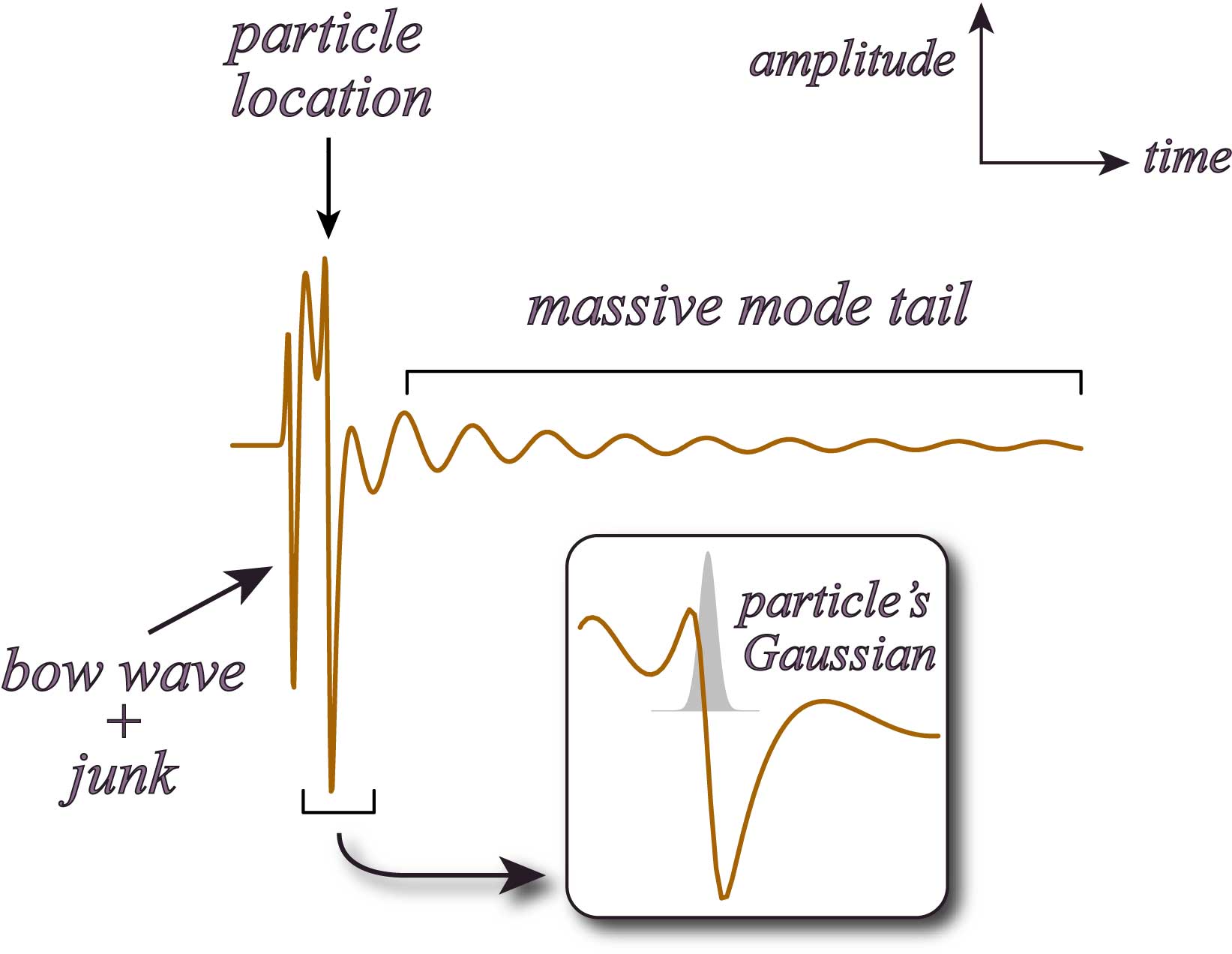
Figure 2: Waveform of a particle moving past an observer in the far field.

There are three key features. The first is the bow wave which precedes the particle: this is just junk from the initial data which we want to minimise. This junk will not interfere with the signal from the particle interacting with the black string, provided we start the simulation when the particle is in the far field: in this case, the spike from the particle increases by over an order of magnitude by the time it gets to $x\approx 30$, dwarfing any contamination from the junk.

The second feature is the particle passing the observer: the disturbance may be compared to the width of the Gaussian, whose FWHM is displayed by the width of the stem of the arrow pointing to it (and is thinner than the width of the line displaying the signal). We can see that the disturbance length scale is much wider implying that the Gaussian is thin enough. The main part of the signal is the massive mode tail which exists in the particle’s wake. This has a characteristic power law decay discussed above; this part of the signal causes problems later as typically it will not have decayed away by the time the signal from the black string reaches the observer, for interesting observer locations (we shall see that interesting signals occur relatively near the black string, so this has ramifications later).

VIII.1 Plunge orbits and the hierarchy of massive modes

We shall investigate here in some detail the situation of a plunge orbit depicted in Fig. 3, with $\epsilon=.1$ and $p=3.09$ (which corresponds to $E=2.0,L=9.78$).

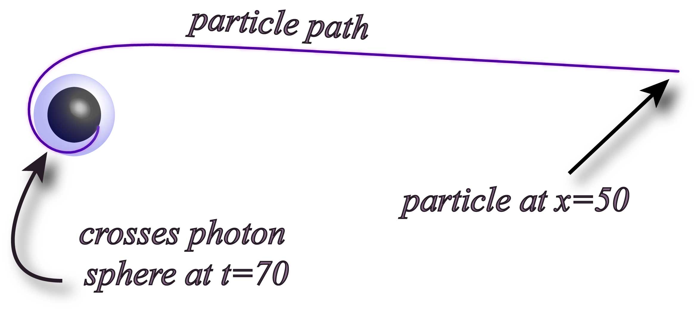
Figure 3: Schematic of our plunge orbit.

We shall show how the hierarchy of mass modes contribute to the total spherical signal. Assuming we are in the “light mode” regime $m_{n}\ell\ll 1$, the KK masses are given by

$$\mu_{n}=[1,1.831,2.655,3.477,\ldots]\mu_{1}.$$ (125)

The string of KK masses we shall use has $\mu_{1}=0.5$, which starts just above the GL instability, where $\mu_{GL}\approx 0.4301$. For $d/\ell=20$ this corresponds to a black string of mass $4.3M_{\odot}$, while for $d/\ell=35$, we have a $1.4\times 10^{9}M_{\odot}$ black string. We will present composite solutions for $\psi$; i.e.,

$$\psi(t,x)=\sum_{n}(z^{+}_{n})^{2}\psi_{n}(t,x),$$ (126)

where $\psi_{n}$ is the numeric solution for a given mass $\mu_{n}$ and the $z_{+}$ parameters are given by (60). We have assumed that both the observer and the source are on the visible brane. Note that if we wanted to reconstruct the full spherical GW signal, we would first have to apply the inversion formulae (106) to each of the $\psi_{n}$ to get $h_{\alpha\beta}^{(n,s)}$ [c.f. (95)] and then sum over $n$ using (89) to obtain the spherical part of $h_{AB}$. However, the simplified composite signal given above will capture most of the essential features of the complete spherical GW signal, and will be sufficient for the qualitative discussion given here.

We show, in Fig. 4, the composite signal $\psi$, and the brane-bending contribution $\xi$, as seen by an observer at $x=100$ for this plunge orbit, starting when the particle passes the observer at $\tau=0$. The integration was started with the particle located at $x\approx 240$, so initial data problems give a very small contamination of the signal, and we have used $\varepsilon=1/3$.

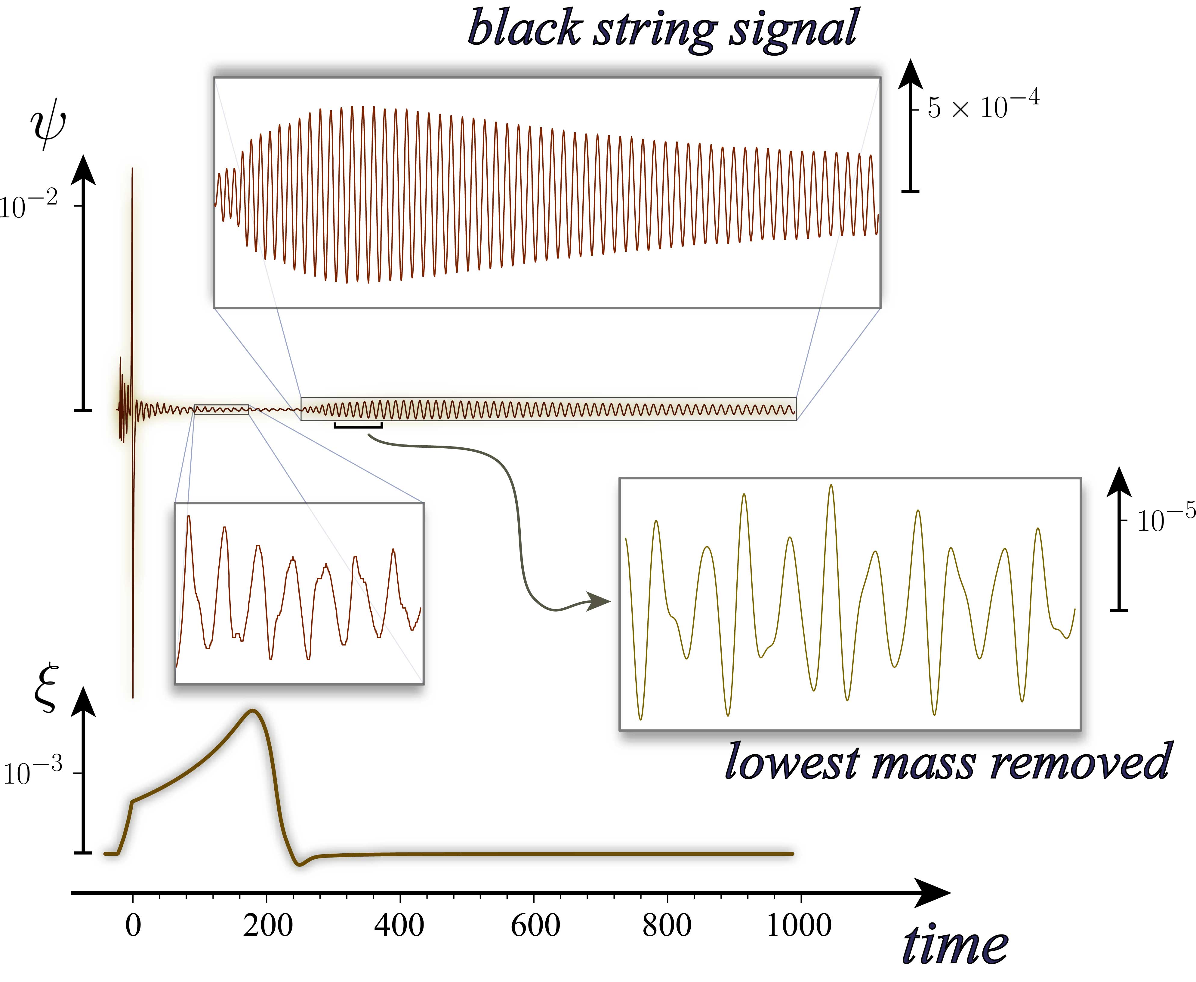
Figure 4: Composite signal from a plunge orbit (top) with brane bending contribution (bottom) for an observer at $x=100$, for the first 4 mass modes.

The gravity wave signal, $\psi$, has two distinct parts. The first, as we have discussed, is from the particle itself and the wave-tail it leaves in its wake. But now we have contributions from higher mass modes, which give a distinct wobble to the tail, shown in the bottom left blow-up. The second is from the black string itself (upper blow-up). As the particle falls into the black string it emits radiation which in the frequency domain is sharply peaked about the frequency of the massive mode (of which more later). Being massive, much of this radiation falls into the string, but some of it makes it out to the observer, the first hint of which arrives around $\tau\approx 300$. This signal reaches a peak around $\tau\approx 4-500$ – a considerable length of time compared to a comparable GR signal – and then gently turns into the characteristic power-law tail fall-off. A key feature of this is the lack of influence the higher mass modes have, compared to $\mu_{1}$; the signal with $\mu_{1}$ removed is shown in the blow-up at bottom right. We can see from the relative scales that this is suppressed by nearly two orders of magnitude. Compare this to the earlier tail from when the particle passes the observer – massive modes higher than $\mu_{1}$ are clearly visible there. The conclusion of this is that signals arising from excitations of the string itself are overwhelmingly dominated by the lowest mass mode.

The overall amplitude of the excitation is worth noting: $\psi_{\mathrm{max}}\sim 5\times 10^{-4}$. Given that the source term from the particle is $\mathcal{O}(1)$, one might naively expect a signal of comparable strength – indeed, this is roughly what happens in GR. Such a weak excitation clearly indicates that spherical massive modes are only weakly stimulated by the particle in-fall. In part this is due to the fact that some of the signal falls into the string; more on this later.

Finally, we come to the composite brane-bending contribution to the signal. The signal, which is independent of $\mu$, is pretty featureless. As the particle passes, a dent in the brane accompanies it; this reaches a peak after the particle has passed, and slowly relaxes back to zero without oscillating. As the brane remains significantly bent long after the particle passes, this extends the total source feeding the gravity wave signal beyond the particle’s Gaussian. Thus, the black string gets a far longer stimulation than it would otherwise get from a point source: the brane bending signal is partly responsible for the length of time $\psi$ remains peaked in the latter part of the signal. This may be seen by the fact that the tail part of the signal has a power-law fall off of $\alpha\approx 1.1$ at $\tau\approx 1000$, so hasn’t yet reached the asymptotic late time value of $5/6$. However, comparison of the signal with the brane bending switched off reveals that the contribution to the amplitude is only of the order of a few percent.

VIII.2 Bound flower-shaped orbits: steady state waveforms

Let us now investigate the signal which comes from a bound orbit, illustrated in Fig. 5, and explore how the signal changes with distance from the black string. We concluded from the previous section that the higher mass modes add only a small correction to the full signal, so here we shall only investigate the signal arising from the lowest mass, $\mu_{1}=0.5$. We choose an orbit with $e=0.5,p=7.05$, and we take $\varepsilon=1$.

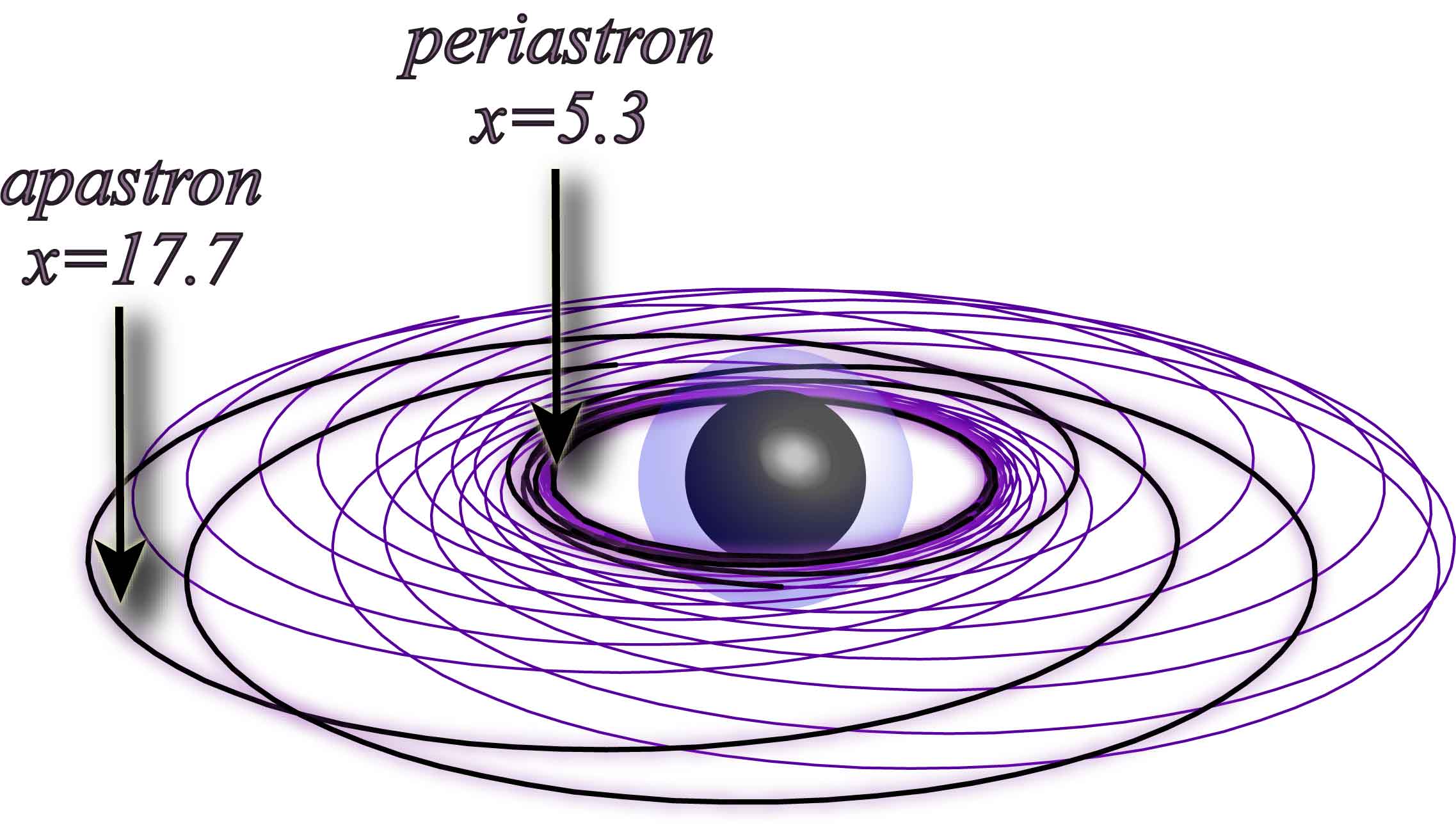
Figure 5: Illustration of the flower-shaped bound orbit used for investigating the steady state waveforms

Integration of the equations is complicated by initial data, once again, but more-so than in the plunge case. This is because the amplitude of the source in the wave equations increases with decreasing $x$, so the best we can do is start the integration at the apastron where it’s smallest, and wait for the contamination to pass the observer. Unfortunately the wave tail makes this quite a long time – roughly $\tau\sim 4-5000$ for an observer around $x\lesssim 100$, compared to $\tau\sim 100$ in GR. After this time the desired steady-state waveform is reached, which we set to $\tau=0$.

In Fig. 6 we show the results of this integration for several observer locations.

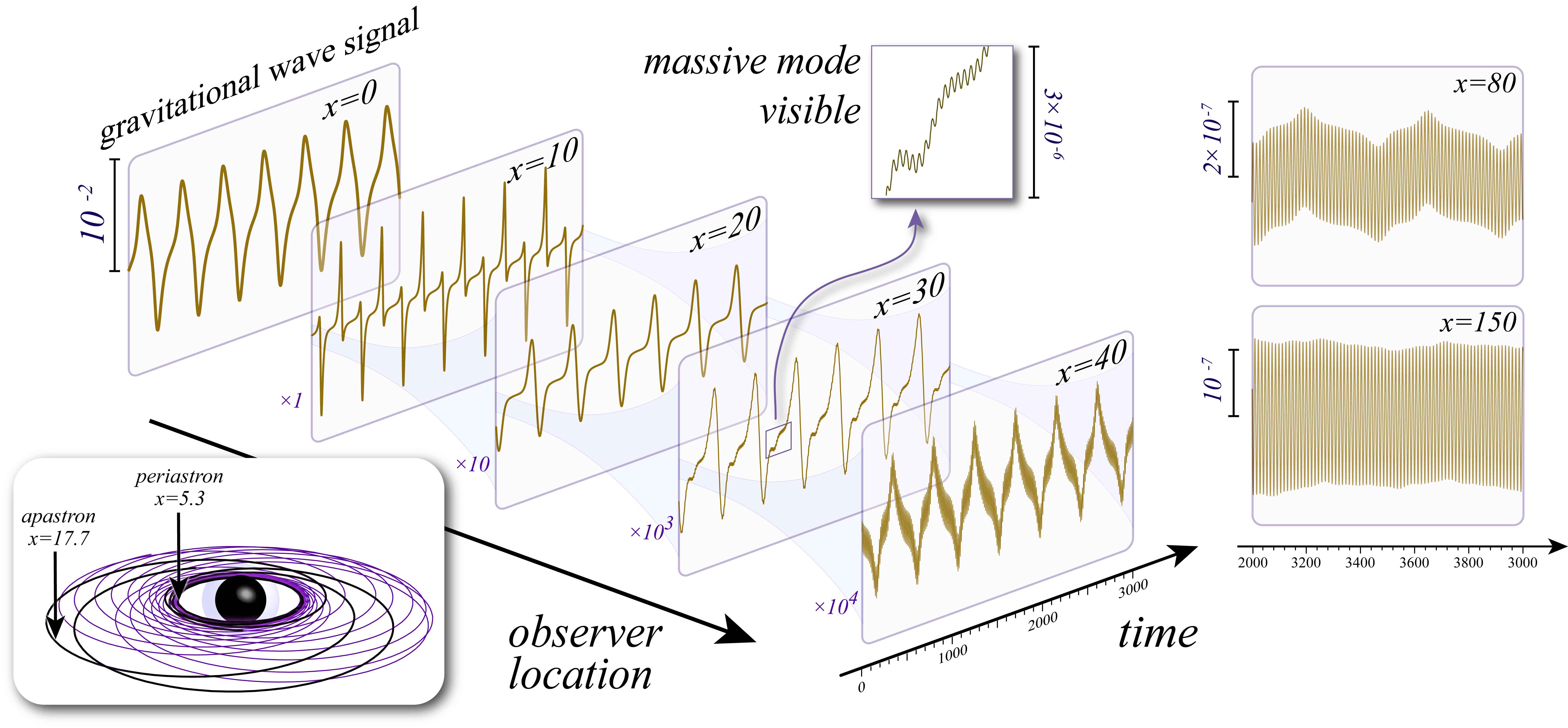
Figure 6: The steady-state gravity wave signal $\psi$ as seen by successively distant observers from the black string, for the lowest mass mode.

As the source evolves it oscillates along the $x$ direction, between about $5.3$ and $17.7$. It can be immediately seen that observers see radically differing signals depending on whether they are in the near, intermediate, or far zones.

Near Zone:

An observer sitting near the photon sphere around $x=0$ will see a relatively normal signal: a gravity wave propagating at light speed (since $V\approx 0$ there) which precisely mimics the behaviour of the source. Around $x=10$ – located in the ‘middle’ of the orbit – the amplitude of $\psi$ reflects the source passing back and forth.

Intermediate Zone:

Here things get a bit more interesting. As we move further out to $x\sim 40$ the direct orbital signal gets damped dramatically – by 4 orders of magnitude. This is due to low frequency parts of the signal being exponentially damped as they travel through the potential (all frequencies roughly less than $\mu$ get damped). By $x\sim 30$ the massive modes become visible as a high frequency wobble riding on the orbital part. And around $x\sim 40$ the two components become equally dominant.

Far Zone:

As we observe from more distant locations where the potential is almost flat virtually all the low frequency components have been suppressed, and we are left with a low amplitude massive signal. A gentle oscillation to the envelope is all that remans of the orbital signal.

One of the interesting and unexpected things about this is that the massive modes are excited at all given that the frequency of the source is orders of magnitudes smaller than the mass. Also note that the amplitude of the signal falling into the black string is about five orders of magnitude larger than the signal which makes it out.

VIII.3 Flyby orbits

Finally we shall consider the case of unbound orbits with high angular momentum. We choose an orbit with $e=3.0$ and $p=12.00001$ (see Fig. fig:fly). This completes about four orbits of the black string, very nearly touching the photon sphere at is periastron ($\tau=0$ in this simulation).

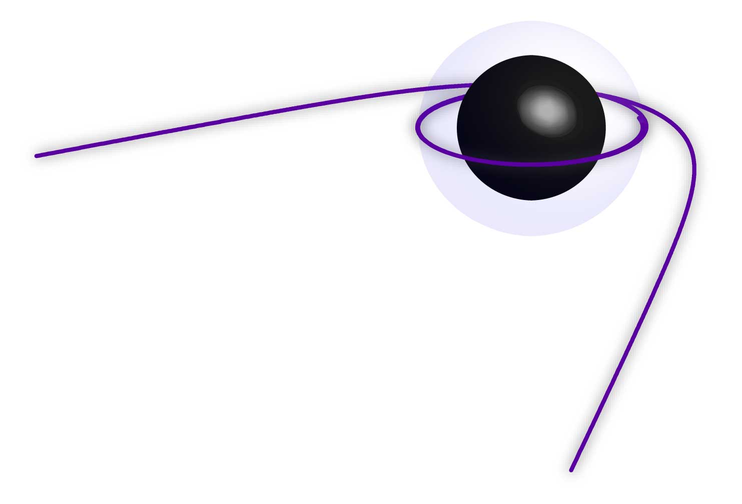
Figure 7: Schematic of the fly-by orbit.

If we think of this orbit in terms of the $x$ coordinate, the particle comes in on a nearly null ray, decelerates very rapidly to zero at the photon sphere where it lingers for $\tau\sim 150$. It then rapidly accelerates off to infinity (of course the particle is geodesic so experiences no acceleration). The source in the wave equation becomes very large at these two events. We see in Fig. 8 how this acceleration can induce a strong GW signal.

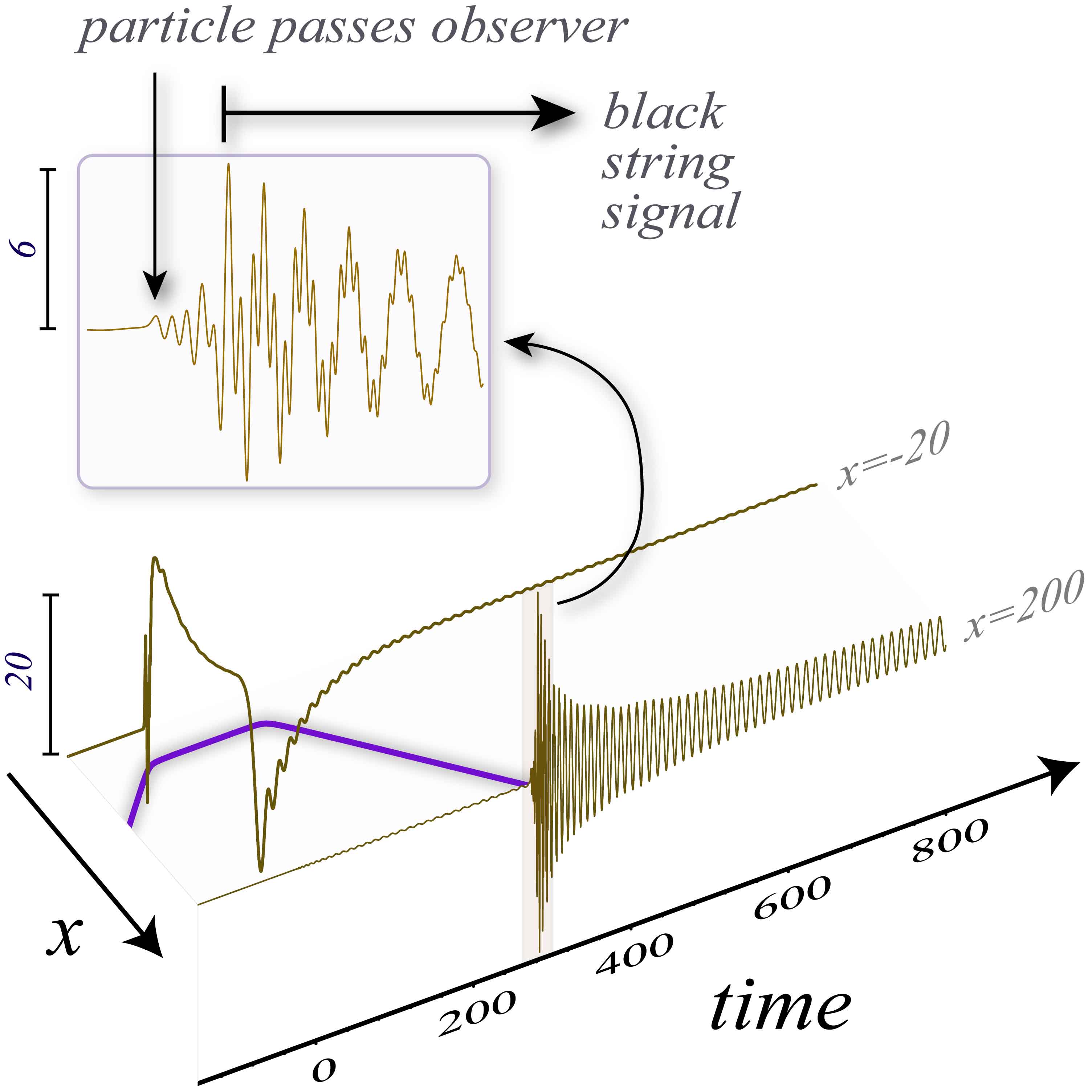
Figure 8: The GW signal from a fly-by orbit, for the lowest mass mode.

First consider the GW which falls into the string. This consists of two pulses corresponding to these two accelerations. As the potential is basically flat in this zone the pulses reflect closely the time evolution of the source. We can see some massive modes on top of this caused by a reflection off the potential.

In the far zone, on the other hand, only the second acceleration produces a GW signal – and this is of nearly the same amplitude as the signal which falls into the string. In the previous two examples the far zone signal was orders of magnitude smaller than that which passes the horizon. The burst of GW seen at $x=200$ nearly coincides with the passing of the particle, although the blow-up shows the the particle precedes the signal somewhat. The peak part of the signal has some interesting wobbles; after this the waveform takes its familiar shape of a decaying massive mode.

The interesting aspect of this simulation is that the amplitude is orders of magnitude larger than the previous two cases. We can understand why this happens by examining the source term, given by Eqs. (120). The two terms which are most important are the coefficients of $\delta^{\prime}[\rho-\rho_{p}(\tau)]$. This is proportional to $u^{r}$, which when $E$ and $L$ are large scale like $(p-3-e^{2})^{-1/2}$ ($=10^{2}$ for the simulation above); thus when $p\rightarrow 3+e^{2}$ we have an infinite source and signal. Note that $u^{r}=0$ at the periastron, so the source peaks near the periastron, when $r$ is small, but not far away when $1/r$ terms kick in. We have numerically confirmed that the signal which makes it to infinity does in fact scale in this way.

IX Discussion

In this paper, we have presented the derivation and numeric solution of the equations of motion for gravitational waves in the black string braneworld sourced by brane localized matter. In §II, we presented a generalized two brane Randall-Sundrum model and then specialized to the black string background. In §III, we considered the linear perturbations of the model and the introduced the Kaluza-Klein massive mode decomposition §IV. The limit under which the model reduces to Brans-Dicke theory was discussed in §V, which led to a constraint on the brane separation. We discussed the specialization of the formalism to spherical radiation (§VI) and pointlike sources (§VII). Finally, in §VIII we presented the results of numeric simulations of the spherical GWs produced by perturbing bodies undergoing plunge, bound, and fly-by orbits.

Future work on this model involves improving our simulation techniques by incorporating characteristic integration techniques Seahra (2006) that more naturally deal with the delta-functions in the GW source. It would also be interesting to consider more realistic modeling of sources of finite size. Once this is accomplished we can build up a bank of simulations for a variety of orbital parameters, choices of $\mu$, and other multipoles. One can then systematically begin looking for these waveform in the data obtained from gravitational wave detectors, and thereby provide a means of further constraining the Randall-Sundrum braneworld model.