Characterization of Chaotic Motion in a Rotating Drum

Abstract

Numerous studies have demonstrated the potential for simple fluid plus particle systems to produce complicated dynamical behavior. In this work, we study a horizontal rotating drum filled with pure glycerol and three large, heavy spheres. The rotation of the drum causes the spheres to cascade and tumble and thus interact with each other. We find several different behaviors of the spheres depending on the drum rotation rate. Simpler states include the spheres remaining well separated, or states where two or all three of the spheres come together and cascade together. We also see two more complex states, where two or three of the spheres move chaotically. We characterize these chaotic states and find that in many respects they are quite unpredictable. This experiment serves as a simple model system to demonstrate chaotic behavior in fluid dynamical systems.

I Introduction and Prior Work

Prior experiments and simulations have shown that particles interacting with fluids can behave chaotically. Simple fluid flows with nonspherical particles nonspherical ; spheroids , stirred particle-filled fluids advection , and various other hydrodynamic interactions reviewchaos can all produce chaotic behavior. In this manuscript, we look at chaotic behaviors involving particles in a horizontal drum which cascade under the influence of a constant external force (i.e. gravity), as first studied by Mullin et al. drumchaos .

In the study of classical Newtonian chaotic systems, there are several heavily studied systems which serve as examples to which other systems can be compared. Simple experiments such as a forced pendulum chaospendulum are easily constructed laboratory experiments which can be studied in depth to better understand low dimensional chaotic behavior. Fluid systems, while containing many more degrees of freedom, also exhibit several geometrically simple experiments which can produce interesting results, giving us insight into the character of chaotic fluid dynamical systems vanhook97 . Relevant to this manuscript, consider non-Brownian particles sedimenting under the influence of gravity. When many particles sediment, interesting swirling motions are seen segre97 . When only a few particles sediment interesting effects are still seen, including chaotic behavior expersed ; stokeslet . Specifically, if three particles are released close to each other, two of the particles eventually pair up and travel together, while the third particle moves on its own isolated trajectory. Intriguingly, this pairing is sensitive to initial conditions. A slight change in the initial particle positions can lead to a switch of which particle is isolated.

These simple sedimentation experiments have only transient chaotic behavior which is difficult to study experimentally. By considering motion in a rotating drum, particles can interact repeatedly, leading to longer-lasting and potentially persistent chaotic behaviors. In a rotating drum partially filled with a liquid and particles, segregation eventually occurs acrivos99 ; acrivos99b . In a purely granular system (no added liquid), similar segregation is also seen choo97 ; choo98 ; williams76 ; bridgwater76 ; hill94 ; hill97 . A simpler system was devised by Mullin et al., in analogy with the three-particle sedimentation simulations of Ref. stokeslet . They studied a hollow cylinder, filled with glycerine, oriented horizontally, and rotated at various angular speeds $\omega$ drumchaos . Three large non-Brownian spheres are placed in this drum. This system serves as a version of a simple sedimentation experiment, with the constraint that the rotation of the drum forces the three beads to remain close together, continually interacting. Figure 1 shows a sketch of this experiment. When the drum rotates, these beads can undergo a periodic cascade in the vertical direction. As they cascade, the beads experience long-range interactions due to the fluid. Mullin et al. found several different behaviors depending on $\omega$. Simple behaviors included states where the three particles remain well-separated and cascade independently of each other. More complex behaviors were observed, such as a state described as “chaotic” where the particles move back and forth horizontally along the tube as they continue to tumble vertically. These horizontal motions were slow, erratic, and unpredictable. In some cases two particles even momentarily collide before withdrawing. No chaotic behavior was observed when there were only one or two beads.

Figure 1: Sketch of rotating drum filled with viscous fluid and three beads. These beads are dragged upwards by the front wall of the drum until gravity pulls them away from the wall and they fall through the fluid. (Based on Ref. drumchaos .)

Motivated by Ref. drumchaos , we study a similar experimental system of a rotating drum with three spheres. The benefit of this experiment is that it can be stably run for very long periods of time, thus allowing us to study the motions of the spheres over a long period of time and describe the chaotic states in great detail (which was not done in Ref. drumchaos ). We find the states seen in Ref. drumchaos as well as three new states. Additionally, we characterize the chaotic states, finding that different chaotic states at different rotation rates $\omega$ often have widely different behaviors, despite a superficial similarity. We thus demonstrate and characterize a simple system which possesses a wide range of nontrivial behaviors.

II Experimental Methods

II.1 The Drum

The experimental apparatus is a $l_{c}=25$ cm long horizontally oriented sealed drum, with an inner radius $r_{c}=5.72$ cm. These dimensions are similar to those used in Ref. drumchaos ($l_{c}=25$ cm and $r_{c}=5.9$ cm). The main body of the drum is constructed from a section of acrylic glass pipe with a wall thickness of 1 cm. To each end of this drum, waterproof threaded aluminum caps are fitted. Each cap has a shaft attached via an adjustable mounting, so that the shaft can be carefully centered within the cap. These shafts attach to a stand via two bearings, which allow the drum to rotate freely about the horizontal axis. The base of the drum stand contains four adjustment screws for leveling the apparatus.

On one of the drum shafts, a pulley is mounted, and connected via a belt to a Dayton 1/2 HP 3-phase A/C motor driven by a Fuji AF-300 controller. This allows the drum to rotate on its axis at a variable rotation rate $\omega$ from $5-13$ rad/s. Due to the belt drive connection, the actual motor rotation rate is potentially different from that displayed on the control box, so the rotation rate of the drum is measured independently using a Pasco PS-2120 rotary motion sensor connected to a computer. Measurements taken over four hours show the rotation rate to be stable to within $1\%$. As all experiments are started from rest, we also measure the time for the drum to spin up to within $1\%$ of its final velocity, and find typical spin-up times to be on the order of tens of seconds.

The drum is filled with $99.5$% pure glycerol from Sigma-Aldrich, and three 440c stainless steel ball bearings purchased from Winstead Precision Ball Company, each of which has a diameter of $2r_{b}=1.59$ cm, density $\rho_{b}=7.65\times 10^{3}$ kg/m³, and mass of $16.1$ grams. When immersed in glycerol ($\rho_{f}=1.26\times 10^{3}$ kg/m²), the beads have an apparent buoyant weight of $0.131$ N each.

To maintain constant viscosity, we control the temperature of the fluid within the drum shankar94 . To do so, we immerse the drum in a tank of water, in which a copper heat exchanger has been placed. We connect this heat exchanger to a Thermo NESLAB RTE-7 digital refrigerated/heated bath, which is maintained at 25^∘ C in all experiments. The rotation of the drum provides sufficient mixing to allow the water within the tank to be maintained at $24.7{\pm}0.1^{\circ}$ C, as measured by a digital thermometer, independently for each experiment. This results in a measured kinematic viscosity $\nu=7.69$ Stokes (as compared with 9.36 Stokes for the fluid used in Ref. drumchaos ).

II.2 Data Collection

To image and track the particles, we use a Pixelink PL-B741F 1.3 megapixel firewire monochromatic camera connected to a personal computer running Windows XP. A Monarch Instruments Nova-Strobe DAX is used to light the particles from behind, which minimizes the motion blur. An opaque screen surrounds the entire apparatus to block ambient light. Compressed movies, lasting up to six hours in duration, were captured using a custom application written in C++ and analyzed with a particle tracking algorithm implemented in Matlab. We can locate particle positions with a resolution of $\pm 0.25r_{b}$, limited by slight optical distortions.

For each experiment, we initialize the particle positions by setting the drum rotation rate $\omega$ to that of a known chaotic state, and stopping the drum when the three beads are distributed equidistant from one another, with approximately 3.5 particle diameters spacing between the beads. The exact rotation rate is not important, as it is simply used as a tool to position the particles. Once the drum is stopped and enough time allowed to elapse for any fluid motion to cease ($\sim 10$ min), we start the rotation of the motor at the desired rotation rate $\omega$, and immediately begin recording video. Videos are streamed directly to the PC hard drive into a compressed Xvid MPEG-4 AVI file. Video files are then post-processed using Matlab. Note that all experiments discussed follow this protocol, starting the drum from rest, setting the speed on the motor for the desired $\omega$, and then turning the motor on. In particular, we do not examine hysteretic effects (although we speculate that there likely are some hysteretic effects, as discussed below).

II.3 Sphere Motion and Nondimensional Numbers

When the drum first begins to rotate, there is a transient state where the fluid is not yet equilibrated to the new rotation rate. This can be estimated by the Ekman pumping time,

$$\tau_{E}=\frac{l_{c}}{\sqrt{\nu\omega}},$$ (1)

based on the cylinder length $l_{c}$, viscosity $\nu$, and final rotation rate $\omega$ spinup . For our experiment, with $\omega\sim 5-13$ rad/s, we have $\tau_{E}\sim 2.4-3.7$ s. This is faster than the time needed for the motor to reach full speed (tens of seconds as noted above), and so the motor is the limiting factor in reaching the steady state. This implies that the behavior seen in our measurements, lasting several hours in duration, is not dependent on effects from the initial spin-up of the drum fluid. Observations of tracer material within the fluid confirm the short spin-up time. In Sec III.4, we will show that typical time scales for horizontal motion of the spheres ($x$ direction) are $O$(100 s), two orders of magnitude removed from the Ekman time $\tau_{E}\sim 3$ s. The particle turnover time (the time for a single cascade to occur) is of order $\sim 1$ s.

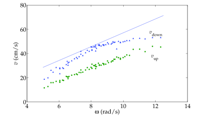
Figure 2: (Color online) Cascade speeds $v_{up}$ and $v_{down}$ plotted versus $\omega$. The solid line represents $v=\omega r_{c}$, showing that $\omega r_{c}$ is an approximate upper bound for the cascade speed.

When we are within the cascade regime, the beads repeatedly cascade in the $y-z$ plane, being dragged up the front wall of the cylinder, then falling away from it. We measure the average speed of the spheres as they rise and fall, and plot these speeds as a function of $\omega$ in Fig. 2. The solid line drawn at $v=\omega r_{c}$ is an approximate upper limit to the characteristic speed $U$ of the particles. Using this, we can compute the particle Reynolds number $Re=UL/\nu$, which determines the contribution of fluid inertial effects relative to viscous drag. Using the bead radius to set the characteristic length scale $L=r_{b}$, the Reynolds number is drumchaos :

$$Re=\frac{\omega r_{c}r_{b}}{\nu}.$$ (2)

Noting that, for this experiment, $r_{c}$, $r_{b}$, and $\nu$ are all fixed, we can write a simple linear conversion

$$Re=0.591\omega\sim 2-8$$ (3)

for the range of $\omega$ we study. These low values of Re correspond to a laminar flow where both viscosity and fluid inertia play a role in the fluid flow. Next, to quantify the importance of viscous forces for influencing the horizontal motions of the beads, we consider the typical viscous damping time $\tau_{\nu}\sim L^{2}/\nu$. Here we use $L=l_{c}$, to quantify interactions across the length of the drum, and find $\tau_{\nu}\sim 80$ s, on the same order as the particle interaction time $\tau_{col}\sim 100$ s.

If we consider the ratio of inertial forces for the particles compared to the fluid, we can typify the relative contributions by comparing the density ratio $\rho_{b}/\rho_{f}\sim 6.2$, which implies that fluid inertia will have less influence upon the bead trajectories than the Reynolds number might otherwise imply. Due to their large inertia relative to the fluid, the beads will not tend to follow fluid streamlines exactly, but rather interact via drag.

Finally, we consider the Galilei number to quantify the ratio of gravitational to viscous forces. The force due to gravity is $F_{g}=(4/3)\pi r_{b}^{3}\Delta\rho g$, and the viscous drag is defined as the Stokes drag $F_{\nu}=6\pi\nu r_{b}U$. Using these we define the Galilei number as masstransfer

$$Ga=\frac{F_{g}}{F_{\nu}}=\frac{2r_{b}^{2}\Delta\rho g}{9\nu U}\sim 1.3-3.9$$ (4)

with $Ga=3.9$ for $\omega=5$ rad/s and $Ga=1.3$ for $\omega=15$ rad/s, using the typical velocity scale as $U=\omega r_{c}$. This shows that the influence due to gravity is always comparable to that due to viscous drag, which is not surprising. At lower rotation rates, the force due to gravity is proportionally larger, meaning the particles will not be lifted up as high in the cylinder ($y$ direction) before falling back down; this is indeed what we observe. Likewise at higher rotation rates, the forces due to gravity and viscous drag are equal in magnitude, and the cascading motion carries the spheres further upward in $y$.

III Results

III.1 Trajectories

In Ref. drumchaos , Mullin et al. describe three types of behaviors for the three bead case. At low Reynolds number (Re $<$ 1.21), they observed fixed-point behavior, where the beads were completely independent of each other. At 1.21 $<$ Re $<$ 2.12, the beads underwent cascading motion in the $y-z$ plane with the $x$ positions fixed, with the axes defined as drawn in Fig. 3. It was noted that as they cascaded, the outer beads were stably out of phase with each other, and the middle bead was at an intermediate position between the two. At Re $=$ 2.12 there was a reversible transition to a chaotic regime where the particles started to wander erratically in the horizontal ($x$) direction while still cascading in the $y-z$ plane. At Re $=$ 4.53, there was a transition to what Ref. drumchaos described as solid body motion. In all cases, the motion in the $y$ direction is always the simple cascading motion, and the motion in $x$ is nontrivial; thus, like Ref. drumchaos , we will focus on the $x$ motion for our analysis.

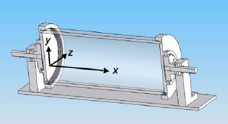
Figure 3: (Color online) The axes are defined such that $x$ represents the horizontal direction, $y$ is the vertical, and $z$ is the depth away from the front edge of the drum. Note that, with our current apparatus, there is no way to measure $z$ directly.

In our experiment, we observed five distinct types of behavior within the cascade regime described by Ref. drumchaos , three of which are new behaviors. At the lowest rotation rates, the three beads simply cascade in the $y-z$ plane with no significant motion in the horizontal ($x$) direction, corresponding to the cascading observations of Ref. drumchaos . Figure 4(a) shows a typical example of this periodic trajectory, at a rotation $\omega=5.31$ rad/s. Each bead appears to move isolated from the influence of the other beads. As rotation rate is increased beyond this initial simple periodic regime, there are several observed types of trajectories, depending on rotation rate. The two simplest of these are also periodic, but to differentiate their unique behaviors we have labeled them as doublet [Fig. 4(b)] and triplet [Fig. 4(c)] states. In the original study drumchaos , neither the doublet nor triplet states were mentioned.

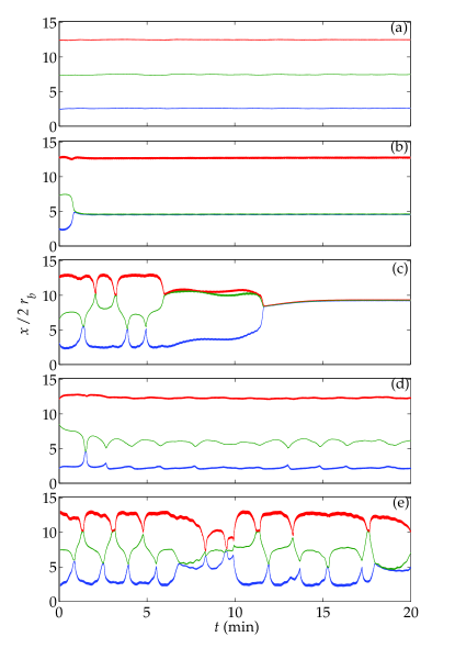
Figure 4: (Color online) Typical examples of trajectories corresponding to the five regimes we observe. (a) Periodic trajectory with $\omega=5.31$rad/s. (b) Stable doublet state with $\omega=7.14$ rad/s. (c) Stable triplet state with $\omega=7.88$ rad/s (d) Biased chaotic state with $\omega=6.56$ rad/s. In such states, the center bead strongly interacts with only one of the outer beads. (e) Fully chaotic state with $\omega=8.51$ rad/s. For all figures, the varying thickness of the lines is a result of particle position uncertainty due to optical distortion from the curved drum walls. This distortion is exaggerated due to parallax near the end caps, and minimized in the center of the drum.

In the doublet state, two of the beads will lock together so that they are cascading in one another’s wakes. The determination of which two beads will tend to pair up is a result of initial conditions, and not a systematic trend in the experimental apparatus. Simply stopping and restarting the drum at the same rotation rate can sometimes switch which two beads will form a pair.

In the triplet state, all three beads come together and cascade in line with one another, in a similar fashion to the doublet state. The three beads can be stacked on top of each other, touching, or they can be spaced out within the drum, following each others’ wakes without touching, depending on whether the beads are closer to in phase or out of phase as they approach one another. Both the doublet and triplet states are stable configurations and have been tested to remain locked for periods exceeding twenty-four hours in duration.

At certain rotation rates, the beads will wander chaotically in the $x$ direction. For chaotic trajectories with a low enough $\omega$, there will be a bias to one side of the drum or the other. This biased chaotic trajectory is illustrated by a typical example as shown in Fig. 4(d). Two of the three beads will tend to repeatedly approach and interact with one another, while the third bead will remain segregated at the far end of the drum. This third bead still experiences long range forces from the other two beads, and can be seen to move in phase with the collisions of the other two. The determination of which two beads will tend to pair up is again seemingly a result of initial conditions, analogous to the doublet state. Like the doublet and triplet states, this biased chaotic behavior was not seen previously drumchaos .

For higher $\omega$ chaotic states, the beads explore a more rich set of interactions, where they wander somewhat erratically in the horizontal direction, occasionally even colliding with each other. The collisions observed include pair collisions (left-middle and right-middle) as well as triplet-type collisions where all three beads come together. Figure 4(e) shows a typical example of this behavior, which we call the fully chaotic state, similar to the behaviors illustrated in Ref. drumchaos . In pair collisions, beads can be either in phase or out of phase with one another (in the cascading direction). In phase collisions are more direct, with the beads immediately colliding and moving away, while out of phase collisions often involve the beads cascading over one another several times before colliding. Triplet-type collisions generally involve two beads cascading over one another while a third bead approaches and collides with them. Note that when we have out of phase collisions, the two beads have identical $x$ positions for a while; our data acquisition rate is not fast enough to carefully follow their motion in $y$, and we cannot distinguish between the beads at that point. Thus, it is likely that in some cases, the two beads exchange places, but we cannot detect this. For example, in Fig. 4 the middle bead is always drawn with the same color, but it is important to recognize that it is quite possible that the identity of this bead changes at collisions.

III.2 Phase Diagram

To probe the dependence of the particles’ behavior on rotation rate, we recorded sixty-eight videos at rotation rates ranging from 5.1 to 12.3 radians per second. An analysis of these videos allows us to map out a phase diagram as shown in Fig. 5. The colored blocks denote different regimes, and gray blocks represent regimes where there is some overlap of behavior, or transitions between two regimes. The width of these transition blocks is due to uncertainty both due to the measurements themselves, and also to the discrete, digital motor control circuit, which limits the resolution of $\omega$ to 1% as noted in Sec. II.

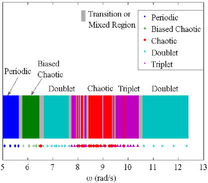
Figure 5: (Color online) Phase diagram showing the behaviors observed at various rotation rates. The symbols below the bar indicate individual observations.

With increasing rotation rate $\omega$, the system undergoes a phase transition from periodic to biased chaotic behavior at $\omega\sim 5.7$, which corresponds to a Reynolds number $\text{Re}\sim 3.4$, comparable to the transition from periodic to cascading motion seen in Mullin et al.’s experiment at $\text{Re}=2.12$ drumchaos . The difference in Re is perhaps due to our different Galilei numbers; because their viscosity was 1.2 times larger than ours, their values for $Ga$ are smaller by that same ratio.

In our observations, the biased chaotic regime is followed by a long doublet regime. After this doublet regime, we find a small window of triplet behavior around $\omega\sim 7.8$ rad/s, which begins a mixed region of behavior, consisting of slices of both chaotic and triplet behavior, extending until $\omega\sim 10.4$. For rotation rates higher than those at which we find triplet behavior, we find reliable doublet trajectories. For high enough rotation rates, we should transition into the motion Mullin et al. described as solid-body drumchaos . We do not probe this regime due to limitations of our motor driving the rotating drum.

This phase diagram illustrates a rich landscape of interesting regimes of particle behavior with a new level of detail. Specifically, Ref. drumchaos identified only one simple, contiguous block of chaotic behavior, while we have identified multiple windows of periodic behavior embedded within large chaotic regimes, as well as previously unidentified periodic behaviors. Furthermore, the distinction between two different types of chaotic behavior illustrates the complexity of the system.

There are two inter-related caveats to be considered when discussing the phase diagram in Fig. 5, transient behavior and motor drift. Transients can pose potential issues in situations where the transients last longer than the duration of an experiment. In a given experiment, after the drum begins rotating, the system takes some time to settle into its long-term behavior. For example, in Fig. 4(c), the particles move back and forth across the drum, colliding several times before finally coming together to form the triplet state at $T\sim 12$ min. In this case, the time is small compared to typical experimental durations ($T\sim 300$ min). However, in other experiments, such as that shown in Fig. 6, transient behavior can persist for longer periods of time. Here, the trajectory is seemingly chaotic for $\sim 120$ min before settling into a stable triplet configuration.

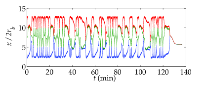
Figure 6: (Color online) In this experiment, at $\omega=8.05$ rad/s, the particle follows a seemingly chaotic trajectory for $\sim 120$ min, but then settles into a stable triplet state.

To further explore the impact of these long transient trajectories, we examine each trajectory and manually determine an approximate transient duration. Figure 7 shows this transient duration plotted versus the rotation rate of the drum. The symbols in the graph represent the type of trajectory found after the transient behavior has died out.

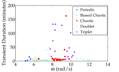
Figure 7: (Color online) The approximate time taken for the initial transient behavior to die out is obtained by eye and plotted versus rotation rate. Symbols represent the long-term phase of each trajectory, after its transients have died out.

Many trajectories have relatively short transient times, with transients rarely exceeding sixty minutes in duration. However, there are also trajectories which contain much longer transient durations, with most of these long-duration transient trajectories clustered around the transitions between different phases. One possible explanation for the long-lived transients is the drum rotation rate, which as Sec. II.1 noted is stable to within $\sim 1\%$. If we consider the transition around $\omega=8$ rad/s, we see that, for a given trajectory, $\omega$ could vary from $7.92$ to $8.08$ rad/s. Thus a possible source for the long transient behaviors is drift in rotation rate of the drum motor. If we imagine small windows of triplet behavior within a chaotic regime, a drum rotation rate which starts within the chaotic regime could drift into the triplet regime, leading to a trajectory which eventually “finds” the triplet state. As already discussed, the triplet state is very robust and stable, and thus once a trajectory finds this state, it would be very difficult to break out of it, even if the rotation rate wanders subsequently. The fact that long transients tend to cluster around the transitions between regimes supports this hypothesis.

This issue of motor drift also has the potential to obscure some detail in the phase diagram. The motor control has finite resolution in available rotation rates, and so there may be small windows of behavior which we are unable to locate. Similarly, even if we did sample these windows, motor drift could take the rotation rate out of a window if it existed within a very narrow range of rotation rates.

III.3 Qualitative Fluid Behavior

To qualitatively describe the fluid flow within the drum, we added a small quantity of Kalliroscope rheological fluid to the glycerol within the drum. Kalliroscope is a water-based suspension of microscopic crystalline platelets. When placed within a moving fluid, the platelets tend to align such that their long axis is parallel to the plane of shear. Thus, the platelets will reflect different amounts of ambient light depending on the local flow of the fluid. This allows us to visualize the flow behavior in each of the states.

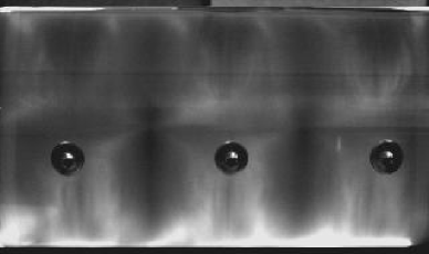
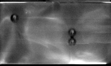
(a) (b) (c)

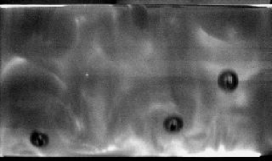
Figure 8: Kalliroscope images show the fluid behavior in various phases: (a) periodic ($\omega=5.31$ rad/s), (b) doublet ($\omega=7.14$ rad/s), (c) chaotic ($\omega=8.51$ rad/s).

Within the periodic regime, the three beads each have a well defined wake, which is bounded on each side by swirling, vortex-like behavior rotating about an axis that extends in the radial direction, as seen in Fig. 8(a). At the midpoints between each pair of particles, there are well defined shear planes which span the entire height of the drum.

In the doublet regime, the two beads which are paired up form a wake which keeps them aligned with one another. This wake is bounded on each side by vortex-like regions where there is swirling fluid flow, as shown in Fig. 8(b). The single bead, well-separated near the far end of the drum, also has a well defined wake, but there is significantly less vortex-like behavior in the fluid.

In the triplet regime , there is one strong wake in which all three beads cascade (not shown). There is a large amount of vortex-like swirling that bounds this wake and likely leads to the observed stability of the triplet state.

The flow within the biased chaotic regime (not shown) appears similar to that within the periodic regime, except when the beads collide. As the beads approach a collision, their wakes overlap and partially merge. At the same time, as the beads are approaching one another, the shear plane that separates them oscillates with greater and greater amplitude, until it breaks up as they approach. After a collision, when the beads are moving apart, the fluid to the outside undergoes a strong vortex-like swirling until the beads are well separated.

Within the fully chaotic regime, the beads’ wakes are often less well defined and more difficult to identify, with large regions of complicated fluid flow, as shown in Fig. 8(c). However, when the beads are well separated, their wakes are evident, with the wakes becoming mixed and obscured as the beads approach one another. The well defined shear planes seen separating the beads in previous cases are not evident in the fully chaotic regime.

In all cases the visualization makes it clear that there is no turbulence, in agreement with the low Reynolds number (Re $\sim 2-8$, see Sec. II.3).

III.4 Timescales

From Fig. 4(e), we note that the particles spend the bulk of their time in a well-separated state where the three particles are spaced far apart in the drum. This configuration is similar to the stable configuration seen in the periodic state shown in Fig. 4(a). Disturbances of the trajectories away from this well-separated configuration are relatively short by comparison. An interesting question, then, is how much time the particles spend in this well separated configuration.

A visual inspection of representative chaotic trajectories seems to indicate a typical time between collisions of the particles. For example, in Fig. 4(d) many of the collisions between particles occur roughly 1-2 minutes apart. Fourier spectra of the $x$ trajectories are noisy and do not depend in any obvious way on the drum rotation rate $\omega$. These Fourier spectra give an indication of typical collision timescales, with typical peak frequencies $f$ between $0.3-1.5$ cycles per minute, with large changes in $f$ at nearly the same $\omega$, corresponding to collision times between $0.6$ and $3.3$ minutes.

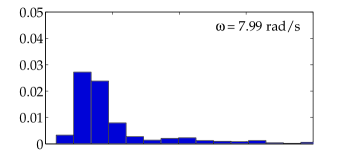
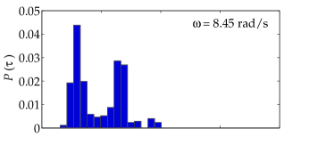
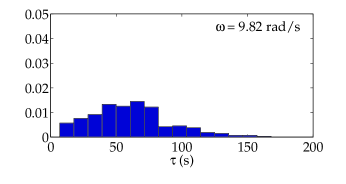
Figure 9: (Color online) Distributions of time between “collisions” where two or three beads come close together. These all correspond to fully chaotic states, with the drum rotation rates as indicated.

To further examine the collision times, we analyzed the time between particle interaction events. To define these events, we note that deviations from the well-separated configuration can be identified by simply looking for local minima and maxima in the trajectory $x_{2}$ of the middle bead. Figure 9 shows the distribution of the time $\tau$ between sequential peaks in $x_{2}$ for three representative experiments within the chaotic regime. There is no simple trend in the shape of these graphs with varying $\omega$. Overall, the distributions of times are all broad with standard deviations comparable to their means, reflecting that the particle trajectories are unpredictable. That is, particles spend a significant time in well-separated positions, and then begin to come together for a collision event after a variable amount of time. Investigation of sequential pairs of dwell times, $\tau_{i}$, $\tau_{i+1}$, showed no structure, further implying unpredictability. The state at $\omega=8.45$ rad/s shows a bimodal distribution, which we observed in only two out of the twenty chaotic states; the other state was at $\omega=8.91$ rad/s, with several uni-modal distributions observed at intermediate values of $\omega$.

III.5 Reduced Dimensionality

To this point, all analysis has focused on the horizontal ($x$) direction trajectories, and neglected cascading in the $y-z$ plane. To further simplify the number of variables used in the data analysis, we sought a reduced dimensionality set of variables which still contains the interesting behavior of the system. We note that, once trajectories have settled into their long-term behaviors, and the transients have died out, the center of mass of the system is constant within the combined noise in the three particle trajectories. This implies that the absolute positions of the particles are not needed to capture the interesting behavior of the system, and we can use a reduced dimensionality to study the behavior. Specifically we use the distances of each outer bead from the center bead:

$$x^{\prime}_{21}=|x_{2}-x_{1}|/2r_{b}$$ (5)

$$x^{\prime}_{32}=|x_{3}-x_{2}|/2r_{b}.$$ (6)

Figure 10 shows a sample trajectory comparing the original coordinates with the reduced coordinates.

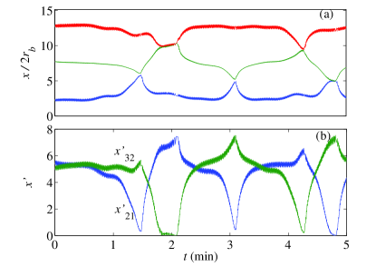
Figure 10: (Color online) (a) Chaotic particle trajectories for an experiment with $\omega=8.79$ rad/s. Recall that we cannot distinguish the spheres from one another, so that by definition $x_{3}\geq x_{2}\geq x_{1}$. (b) The same trajectories in reduced coordinates. The minima in these simplified trajectories indicate points where particle pairs approach one another.

As shown in Fig. 10, there are certain configurations in which the system spends more time, and other configurations that are only visited briefly. Configurations with the three beads well separated appear to be most common, while situations where the beads are close together are shorter-lived. To quantify this, we plot a two dimensional histogram of the configurations, which gives us a way to visualize the relative amount of time each particle spends in various regions of phase space. Histograms are plotted with a logarithmic intensity, so rare events can still be identified. In each experiment, we visually inspect the data set and remove any obvious initial transient behavior manually before analysis. For example, the analysis of a triplet data set only includes the time after the three beads have lined up.

Figure 11 shows an example of one of these histograms for the same experiment shown in Fig. 10. Notice that the darkest red region is in the area around $x^{\prime}_{21}\approx x^{\prime}_{32}\approx 5-6$, corresponding to a configuration where the three beads are spread far apart, and spaced roughly equidistantly. There are also small clusters at $x^{\prime}_{21}\sim 7.5$ and $x^{\prime}_{32}\sim 0$, and its mirror $x^{\prime}_{21}\sim 0$ and $x^{\prime}_{32}\sim 7.5$, which correspond to configurations where two beads are close together, and the third bead is far away. Finally, there is another faint cluster at $x^{\prime}_{21}\sim 0$ and $x^{\prime}_{32}\sim 0$, corresponding to a state where all three beads are grouped together. The faintness of this cluster implies that very little time is spent in this configuration.

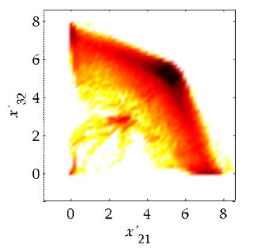
Figure 11: (Color online) A typical two dimensional histogram for a chaotic trajectory at $\omega=8.79$ rad/s. The axes represent the distances between the pairs of particles, normalized by the particle diameter, and color represents the number of points that were counted in each bin. Darker colors indicate more prevalent configurations. This experiment has a calculated entropy $S=6.33$.

The histograms show how the different phases of the system explore phase space. Figure 12(a) shows a schematic of typical histograms for periodic, doublet, and triplet trajectories. Periodic trajectories have well-separated beads and thus the weight of the histogram stays concentrated at point 1. Doublet states have a histogram with points clustered tightly near one of the locations marked 2; for example, if beads 2 and 3 are together in the doublet state, then $x^{\prime}_{23}=0$. In the triplet state, the three beads coincide in their $x$ coordinates and thus the histogram is at the origin, where point 3 is shown. Figure 12(b) shows a biased chaotic trajectory, where the beads spend time in the same region of phase space as the periodic state, but also wander chaotically in the $x$ direction, smearing the histogram in the direction of the bias (in this case, beads 2 and 3 come close together). In Fig. 12(c) we see a chaotic trajectory. The beads explore the phase space around the locations of periodic, doublet, and triplet states [points 1, 2, and 3 in Fig. 12(a)]. Time is also spent in an intermediate configuration ($x^{\prime}_{12}\approx x^{\prime}_{23}\approx 3.5$) where the three beads are closer together than in the periodic trajectory, but not clustered like in the triplet state. This is in contrast to the chaotic state shown in Fig. 12(d), where the beads spend the bulk of their time well-separated, as in the periodic state, with occasional doublet-like collisions. The fact that these states occur at rotation rates which are very similar ($\omega=9.25,9.36$ rad/s) illustrates how sensitive the experiment is to the rotation rate.

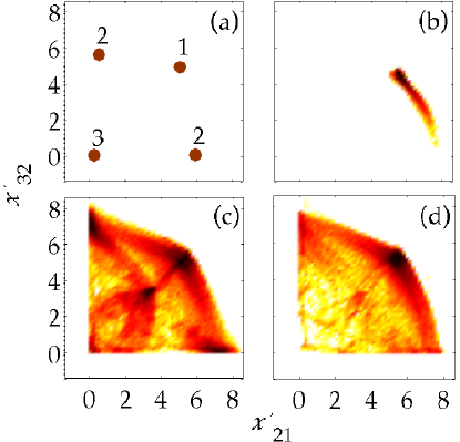
Figure 12: (Color online) Histograms for each phase of behavior clearly illustrate the amount of phase space they explore. (a) Schematic of typical areas occupied by the the non-chaotic trajectories. “Periodic” trajectories such as shown in Fig. 4(a) appear as a tight cluster of points near position 1. “Doublet” trajectories reside at one of the two locations marked as position 2. “Triplet” trajectories have all the particles at the same $x$ position, and thus the histogram for these states is a tight collection of points near the origin, marked as position 3. (b) A histogram for a biased chaotic trajectory at $\omega=6.05$ rad/s. For this state, the entropy $S=3.52$. (c,d) Histograms for chaotic trajectories at $\omega=9.25,9.36$ rad/s, respectively. The entropies of these states are $S=6.82,6.49$.

III.6 Entropy

To quantitatively study the extent to which a given trajectory explores phase space, we define a configurational entropy based on these histograms. If we first normalize a given histogram so that the sum of all bin values is equal to unity, the histogram will represent a probability distribution $P$ with matrix elements $P_{ij}$. We then define the entropy

$$S=-k\sum_{ij}P_{ij}\text{ln}P_{ij}\hskip 7.22743pt,\hskip 7.22743pt\text{with}\ k\equiv 1.$$ (7)

This entropy value is calculated for each individual trajectory and plotted versus rotation rate in Fig. 13. The triplet states have the lowest entropy, followed by the periodic, doublet, biased chaotic, and finally the fully chaotic states with the highest entropy. To quantify error in entropy measurements we split each trajectory into two halves, and calculate the entropies $S_{1}$ and $S_{2}$ for each half independently. Then the error can by defined as:

$$\sigma_{S}=|S_{1}-S_{2}|,$$ (8)

yielding the error bars shown in Fig. 13.

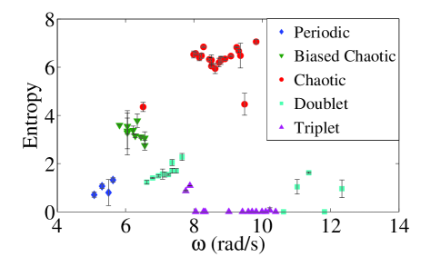
Figure 13: (Color online) The entropy for each rotation rate, calculated from the 2-D histograms.

As could be expected, the entropy is lowest in the simplest states: the triplet, doublet, and periodic states. Nonzero values for the entropy correspond to slight wobbling of the particles around their mean positions in each state. At values of $\omega$ corresponding to transitions between states, Fig. 13 shows sharp changes in the entropy. For example, the biased chaotic state has entropy values markedly higher than the adjacent doublet states. The fully chaotic states have the highest entropy. Within each regime, there can be moderate fluctuations of the entropy values, with little systematic dependence on $\omega$.

Much as the histograms provide a visual indication of the degree to which a trajectory explores phase space, these entropy values provide a qualitative measure of that exploration. Low entropy periodic, triplet, and doublet regimes do not explore phase space much, as expected. Chaotic behaviors, on the other hand, have large entropies, corresponding to extensive exploration of phase space. These entropies vary little by comparison to the large jumps between regimes, indicating that the amount of phase space explored by chaotic behaviors does not vary much with rotation rate.

The magnitude of these entropy values varies with the size of bins used for the histograms. We divide each axis into $60$ divisions, giving a total of $60^{2}$ bins, with each bin having a width $w\sim r_{b}/3$. The qualitative results are unchanged with $40^{2}$ or $80^{2}$ bins.

IV Summary

We have studied a geometrically simple system containing three particles moving within a fluid-filled rotating drum which yields a rich and varied set of behaviors. The phase diagram for this system showed five types of behavior. The first is a periodic regime where the beads simply cascade in the $y-z$ plane. The second is a previously unreported biased chaotic regime where two of the beads wander chaotically in the horizontal $x$ direction and collide with one another. The third is a doublet regime, where two beads pair up and cascade on top of one another while leaving the third bead behind. There is also is a mixed chaotic regime spanning a wide range of rotation rates, where the beads wander chaotically in the horizontal direction, with all three beads interacting and mixing. Within this mixed regime, there are small windows of rotation rates which result in triplet behavior, where all three beads will line up and cascade on top of one another. Finally, we find a regime where triplet behavior is the only type of trajectory seen.

The question of transient behavior deserves significant attention and exploration. We find chaotic states that are persistent over many hours. However, based on similarities between the chaotic states and the transient behavior of the triplet states, it is possible that the chaotic states could eventually fall into a stable triplet state. Our “fastest” observed chaotic states have mean collision times of approximately 0.6 min, and our longest observations are up to 360 min, so at most we have 600 collisions observed in chaotic states without a transition to a triplet state, thus at least showing that if these are transients that they are very long-lived.

Another interesting question is that of dependence on initial conditions. Due to the way the particles were positioned within the drum, it was difficult to control their exact starting positions. However, the long-term statistics of the system’s behavior were reproducible, within the limits of motor drift and transients.

We have also tried preliminary experiments with a longer drum (thus larger aspect ratio), and find that particles prefer doublet or triplet states; we do not see long-lived chaotic states in longer drums. This suggests that a key to the chaotic states is indeed the finite drum size that forces the beads to interact with each other. Overall, we have demonstrated a simple system with complex and chaotic behavior, and furthermore shown that within the previously observed chaotic regime (Ref. drumchaos ) there is a richness of behavior with the “degree” of chaos changing dramatically with only slight changes of rotation rate.

- (1) H. Shin & M. R. Maxey. “Chaotic motion of nonspherical particles settling in a cellular flow field.” Phys. Rev. E, 56, 5341–5443 (1997).
- (2) Anil, Satheesh, & T. R. Ramamohan. “Chaotic dynamics of periodically forced spheroids in simple shear flow with potential application to particle sedimentation.” Rheological Acta, 34, 504–511 (1995).
- (3) H. Aref & S. Balachandar. “Chaotic advection in a stokes flow.” Phys. Fluids, 29, 3515–3521 (1986).
- (4) K. Asokan, Anil, J. Dasan, K. Radhakrishnan, Satheesh, & T. R. Ramamohan. “Review of chaos in the dynamics and rheology of suspensions of orientable particles in simple shear flow subject to an external periodic force.” J. Non-Newtonian Fluid Mech., 129, 128–142 (2005).
- (5) T. Mullin, Y. Li, D. C. Pino, & J. Ashmore. “An experimental study of fixed points and chaos in the motion of spheres in a stokes flow.” IMA Journal of Applied Mathematics, 70, 666–676 (2005).
- (6) D. D’Humieres, M. R. Beasley, B. A. Huberman, & A. Libchaber. “Chaotic states and routes to chaos in the forced pendulum.” Phys. Rev. A, 26, 3483 (1982).
- (7) S. J. Van Hook & M. F. Schatz. “Simple demonstrations of pattern formation.” The Physics Teacher, 35, 391–395 (1997).
- (8) P. N. Segrè, E. Herbolzheimer, & P. M. Chaikin. “Long-range correlations in sedimentation.” Phys. Rev. Lett., 79, 2574 (1997).
- (9) K. O. L. F. Jayaweera, B. J. Mason, & G. W. Slack. “Behavior of small clusters of spheres falling in a viscous fluid.” J. Fluid Mech, 20, 121 (1964).
- (10) I. M. Jánosi, T. Tél, D. E. Wolf, & J. A. Gallas. “Chaotic particle dynamics in viscous flows: The three-particle stokeslet problem.” Phys. Rev. E, 56, 2858 (1997).
- (11) M. Tirumkudulu, A. Tripathi, & A. Acrivos. “Particle segregation in monodisperse sheared suspensions.” Phys. Fluids, 11, 507–509 (1999).
- (12) M. Tirumkudulu, A. Tripathi, & A. Acrivos. “Erratum: “particle segregation in monodisperse sheared suspensions” [phys. fluids [bold 11], 507 (1999)].” Phys. Fluids, 11, 1962 (1999).
- (13) K. Choo, T. C. A. Molteno, & S. W. Morris. “Traveling granular segregation patterns in a long drum mixer.” Phys. Rev. Lett., 79, 2975–2978 (1997).
- (14) K. Choo, M. W. Baker, T. C. A. Molteno, & S. W. Morris. “Dynamics of granular segregation patterns in a long drum mixer.” Phys. Rev. E, 58, 6115–6123 (1998).
- (15) J. Williams. “The segregation of particulate materials. a review.” Powder Technology, 15, 245–251 (1976).
- (16) J. Bridgwater. “Fundamental powder mixing mechanisms.” Powder Technology, 15, 215–236 (1976).
- (17) K. M. Hill & J. Kakalios. “Reversible axial segregation of binary mixtures of granular materials.” Phys. Rev. E, 49, R3610–R3613 (1994).
- (18) K. M. Hill, A. Caprihan, & J. Kakalios. “Bulk segregation in rotated granular material measured by magnetic resonance imaging.” Phys. Rev. Lett., 78, 50–53 (1997).
- (19) P. N. Shankar & M. Kumar. “Experimental determination of the kinematic viscosity of glycerol-water mixtures.” Royal Society of London Proceedings Series A, 444, 573–581 (1994).
- (20) E. R. Benton & A. Clark. “Spin-up.” Annual Review of Fluid Mechanics, 8061, 257–279 (1974).
- (21) H. D. Baehr & K. Stephan. Heat and Mass Transfer (Springer) (2006).