Liquid polymorphism, order-disorder transitions and anomalous behavior:
a Monte Carlo study of the Bell-Lavis model for water

Abstract

The Bell-Lavis model for liquid water is investigated through numerical simulations. The lattice-gas model on a triangular lattice presents orientational states and is known to present a highly bonded low density phase and a loosely bonded high density phase. We show that the model liquid-liquid transition is continuous, in contradiction with mean-field results on the Husimi cactus and from the cluster variational method. We define an order parameter which allows interpretation of the transition as an order-disorder transition of the bond-network. Our results indicate that the order-disorder transition is in the Ising universality class. Previous proposal of an Ehrenfest second order transition is discarded. A detailed investigation of anomalous properties has also been undertaken. The line of density maxima in the HDL phase is stabilized by fluctuations, absent in the mean-field solution.

I Introduction

Water is probably the most familiar substance in nature, due to its abundance and relevance for the existence of life. It exhibits sixty-six thermodynamic, dynamic and structural properties recognized to be anomalous URL , that is, unusual when compared with the behavior of other substances. The most familiar anomaly is the increase of density with temperature, at ambient pressure, up to $4^{\rm o}{\rm C}$. Above this temperature water behaves as a normal liquid and density decreases as temperature rises. Experiments for water allow to locate the line of temperatures of maximum density (TMD), below which the density decreases with decreasing temperature, differently from the behavior of the majority of fluids, for which density increases on lowering temperature An76 .

In order to explain the thermodynamic anomalies, it has been proposed that these anomalies could be related to a second critical point at the end of a coexistence line between two liquid phases, a low density liquid (LDL) and a high density liquid (HDL) Po92 . In spite of its experimental inaccessibility, due to its localization beyond the line of homogeneous nucleation, in the supercooled region, the experimental indication of the presence of polymorphism in the same region and results from numerical experiments on realistic water models have maintained the idea of a second critical point alive.

Water, however, is not an isolated case. There are also other examples of tetrahedrally bonded molecular liquids such as phosphorus Ka00 ; Mo03 and amorphous silica La00 that are other good candidates for having two liquid phases. Moreover, other materials such as liquid metals Cu81 and graphite To97 also exhibit thermodynamic anomalies. Unfortunately a coherent and general interpretation of the low density and high density liquid phases is still missing. Despite the lack of consensus concerning the origin of water-like anomalies, it is widely believed that they are related to the hydrogen bond. The tetrahedral structure of ice is a consequence of hydrogen bonding which is responsible for ice being less dense than the liquid phase. By increasing temperature, latent heat is used up to disrupt hydrogen bonds which allows molecules to get closer. Thus density increases as temperature rises, up to the temperature of maximum density (TMD). As temperature rises further, most of the hydrogen bonds are broken and water behaves as a normal fluid, i.e., the density decreases by increasing temperature.

A variety of statistical models have been proposed in order to reproduce the main features of liquid water, and specially its anomalies. From a general point of view, statistical models can be classified into isotropic and orientational models. The first class of models has focalized on the density anomaly and its possible relation to the existence of two characteristic lengths with an usual attractive interaction and a soft repulsive interaction. The competition between these lengths gives rise to anomalies Ol06a ; Ol06b ; Wi01 ; He70 ; Ja99a ; Ca03 ; Ku05 ; Ne06 ; Ba04 ; Ol05 . Another class of isotropic models is that in which the particles are represented by lattice gas variables and each particle has bonding variables represented by Potts-like states. The density anomaly is introduced ad hoc by the addition to the free energy of a volume term proportional to a Potts order parameterSa93 ; Sa96 ; Fr03 .

One example of orientational model, studied both in two Pa99 and three Ro96 dimensions also has bonds represented by Potts variables but the number of bonds is limited by an energy penalty when a neighbor site to a bond is occupied. This is also the mechanism for introducing the density anomaly in this model. The second class of orientational model emphasizes the fixed orientation of the hydrogen bond. One example of this type of model was introduced by Bell and and collaborators Be70 ; La73 ; Yo79 ; So80 and imposes a fixed number of possible arm states. Further work on analogous 3-d orientational models revealed the possibility of a density anomaly Be94 . More recently, Henriques and Barbosa introduced a lattice model in two He05a ; He05b and three dimensions Gi07 where water molecules have four bonding and two inert arms (2-d) and four inert arms (3-d). The anomalies appear due to the presence of two competing interactions: hydrogen bonds and isotropic repulsive van der Waals forces. In the spirit of water interactions, the presence of nonbonding neighbors is punished by an increase of energy.

Although all models mentioned above are able to reproduce water-like anomalies, the understanding of the role played by directionality is still missing. While in water and other tetrahedral liquids directionality seems to play a relevant role, it is not required to reproduce the thermodynamic and dynamic anomalies displayed in the case of isotropic potentials. It was also shown that the for the presence of the anomalies it is not relevant the distinction between the acceptor and donor arm in the hydrogen bond Ba07 .

Which would be the contribution of the directionality in these models? In order to answer this question in this paper we explore thoroughly the properties of the Bell-Lavis model Be70 . The model is the only 2d orientational model known to us which does not require an energy penalty in order to present a density anomaly. It is a triangular lattice gas model in which water molecules are represented by three symmetric bonding arms and interact through van der Waals and hydrogen bonds.

The phase-diagram of this model has been previously explored by means of mean-field approximations Be70 ; La73 , real space renormalization group analysis Yo79 ; So80 and, more recently, through the cluster variation method Br02 and from Bethe calculations for the Husimi cactus Ba08 . Some Monte Carlo simulations have also been presented by Patrykiejew and co-workers Pa99 . Besides the gas-liquid transition, an open bonded network is exhibited by the model, at lower pressures and temperatures (the low density liquid or open phase), which gives way to a dense poorly bonded network (the high density liquid or full phase). Consensus is lacking on the order of the liquid-liquid transition. The mean-field studies predict a weak first-order transition, whereas the renormalization group and the Monte Carlo simulations suggest a critical transition. The latter also argues for a second order transition of the Ehrenfest type. As to thermodynamic anomalies, these have not been investigated through simulations, and Bethe calculations Ba08 have shown the density anomaly to be metastable.

We also undertake a thorough investigation of the model thermodynamics in order to ascertain the order of the transition, its universality class and the definition of an order parameter. In addition we check for the presence of a stable density anomalous region of the phase-diagram.

This paper is organized as follows: In Sec. II the model is described and the ground state analysis is presented, in Sec. III the simulation results for the model thermodynamics are presented and in Sec IV final comments close the paper.

II The Bell-Lavis model and ground state analysis

The Bell-Lavis model is a two dimensional triangular lattice gas. Particles are represented by occupational variables $\eta_{i}$, with $\eta_{i}=0,1$ for empty or occupied sites, respectively. Each water particle has two orientational states, as can be seen in Fig 1a. Orientation may be described in terms of bonding and non-bonding ”arms”. The latter are represented through variables $\tau_{i}^{ij}$ for the arm of particle $i$ which points to particle $j$. An arm may be non-bonding if $\tau_{i}=0$, or bonding, for $\tau_{i}=1$ (see Fig. 1a and Fig. 1b).

a) b)

Figure 1: Bell-Lavis water model interactions. (a) Two orientations of the water particles: pair interaction energy is $-\epsilon_{vdw}$; (b) water molecules form a hydrogen bond: pair interaction energy is $-(\epsilon_{vdw}+\epsilon_{hb})$

Two next neighbor molecules are considered to interact via van der Waals forces and hydrogen bonds. The model may be described by the following effective Hamiltonian in the grand-canonical ensemble:

$${\cal H}=-\sum_{(i,j)}\eta_{i}\eta_{j}(\epsilon_{hb}\tau_{i}^{ij}\tau_{j}^{ij}+\epsilon_{vdw})-\mu\sum_{i}\eta_{i},$$ (1)

where $\epsilon_{hb}$ is the energy associated with the formation of a hydrogen bond, in case two bonding arms point to each other (see Fig 1b), $\epsilon_{vdw}$ is the van der Waals interaction energy (vdW) and $\mu$ represents the chemical potential. The hydrogen bond interaction tends to make the particle density $\rho$ smaller, in order to make hydrogen bond density larger. This can be seen by inspection of hydrogen bonding on the lattice: the system is fully hydrogen-bonded if the particle arms are oriented such as to form a honey-comb-like structure (see Fig 2a). In this case, particle density is $\rho=2/3$, and the number of hydrogen bonds per particle is $\rho_{hb}=3/2$. On the other hand, the van der Waals interaction and the chemical potential field tend to fill up the lattice. However, if the lattice is fully occupied, $\rho=1$, the number of hydrogen bonds per particle is reduced to $\rho_{hb}=1$ (see Fig 2b). This competition between the van der Waals and the hydrogen-bond interactions yields the possibility of the appearance of two dense phases, with densities $\rho=2/3$ and $\rho=1$, respectively, at low temperatures.

(a) Example of the configuration that represents the LDL phase. Note that it is ordered and presents, in contrast to the HDL phase, only one configuration.

(b) Example of a possible configuration of the HDL phase.

Figure 2: Liquid phases at zero temperature for the BL model.

The existence of two dense phases depends on the relative intensity of the two interactions, $\zeta\equiv\epsilon_{vdw}/\epsilon_{hb}$. At zero temperature, in addition to the gas phase, with $\rho=0$, two dense phases have been proposed for the model system, if $\zeta=\epsilon_{vdw}/\epsilon_{hb}<1/3$: a high density liquid phase, HDL, with $\rho=1$ and a low density liquid phase, LDL, with $\rho=2/3$ Pa99 ; Ba08 . The two phases are illustrated in Fig.2 (a) and (b).

Stability of the three phases can be investigated from analysis of the grand potential. At $T=0$, the reduced grand potential free energy density, $\phi\equiv\Phi/V\epsilon_{hb}$, is obtained from $\Phi=\langle\cal{H}\rangle$. ¿From inspection of the number of nearest neighbors and of hydrogen bonds for each phase (see Fig. 2 ), one may write down the reduced grand potential for the three possible phases as:

$$\phi_{gas}=0$$ (2)

$$\phi_{LDL}=-1-\zeta-\frac{2}{3}\overline{\mu}\;$$ (3)

$$\phi_{HDL}=-1-3\zeta-\overline{\mu};$$ (4)

where $\overline{\mu}=\mu/\epsilon_{hb}$.

As expected, at very low and negative chemical potentials the gas phase dominates. As the chemical potential is increased, the low density liquid phase (LDL) becomes stable, whereas at still larger chemical potentials the high density liquid (HDL) corresponds to the stable phase.

The first phase transition, between the gas and the low density liquid, takes place at chemical potential given by

$$\overline{\mu}_{\scriptscriptstyle{gas-LDL}}=-\frac{3}{2}(1+\zeta),$$ (5)

which is obtained through equating the grand potentials, or pressures, of the two phases, $\phi_{gas}=\phi_{LDL}$. The second phase transition, between LDL and HDL, occurs at $\phi_{LDL}=\phi_{HDL}$, which makes the chemical potential at the transition

$$\overline{\mu}_{\scriptscriptstyle{LDL-HDL}}=-6\zeta.$$ (6)

In the next section we present our simulation studies of the model system properties for finite temperatures. Our interest lies in model parameters which may yield a density anomaly, and we thus look for systems with two dense phases, which implies taking the interaction strength of the hydrogen bond dominating over that of the van der Waals parameter, i.e. $\zeta<1/3$. We have thus focused on two cases, $\zeta=1/4$ and $\zeta=1/10$, which describe, respectively, weaker and stronger hydrogen-bonding with respect to van der Waals, respectively and which we discuss below.

III Thermodynamics: Monte Carlo simulations

Model thermodynamic properties were obtained through careful Monte Carlo simulations.

The microscopic configurations were generated through randomly selected exclusion, insertion or rotation of particles in a grand-canonical ensemble, i.e., for fixed values of temperature and chemical potential. Acceptance rates are those of the usual Metropolis algorithm in the grand-canonical ensemble: transitions between two microstates are accepted according to $\min\{1,\exp(-\beta\Delta{\cal H})\}$, where $\Delta{\cal H}$ is the effective energy difference between the two states. Periodic boundary conditions were adopted. Our simulations were carried out for lattice sizes ranging from $L=30$ to $L=90$.

Densities are calculated as averages, as usual. Obtaining fields is a more delicate task, in simulations. Pressure was evaluated in two independent ways. In the first case, the pressure was computed via numerical integration of the Gibbs Duhem equation, $SdT-Vdp+Nd\mu=0$, at fixed temperatures, namely $dp=\rho d\mu$. Integration was carried out from a sufficiently low density value, at which pressure is zero. In the second procedure, the grand potential free energy $\phi$ is obtained from the largest eigenvalue of the transfer matrix using the Hamiltonian Eq. (1). Since the pressure and the grand potential free energy are related through $p=-\Phi/V$, this is an alternative which allows calculating the pressure directly from the simulations and avoids performing an integration. The method is shown in detail in the appendix A.

III.1 Phase Diagrams: two liquids and order-disorder transition

Phase diagrams in the chemical potential vs. temperature plane are displayed in Figs. 3 and 4 for $\zeta=1/10$ and $\zeta=1/4$ respectively. The pressure vs. temperature phase diagram for $\zeta=1/10$ and $\zeta=1/4$ is shown in Fig. 5 and 6, respectively. Reduced model parameters are used: $\overline{T}=T/\epsilon_{hb}$, $\overline{P}=P/\epsilon_{hb}$ and $\overline{\mu}=\mu/\epsilon_{hb}$. Unless otherwise stated, results presented here are for lattice size $L=42$.

For both interaction parameters analyzed, at low chemical potential and temperature, the system is constrained to the gas phase. By increasing chemical potential for a fixed low temperature, a first order phase transition between the gas and the $LDL$ phase occurs. By increasing further the chemical potential at fixed low temperature a second order phase transition from the $LDL$ to the $HDL$ phase takes place.

At $\overline{T}=0$, the gas-LDL phase transitions take place at $\overline{\mu}_{\scriptscriptstyle{gas-LDL}}=-1.65$ and $-1.875$, for $\zeta=1/10$ and $1/4$, respectively (see Eq. (5)). As to the LDL-HDL phase transition, the corresponding points are $\overline{\mu}_{\scriptscriptstyle{LDL-HDL}}=-0.60$ and $-1.5$, respectively (see Eq. (6)).

The first-order line between the gas and the LDL phases was investigated by means of histograms of density, as shown in Figs. 7 and 8, for smaller and larger vdW strength interactions, respectively. At phase coexistence, one has a bimodal distribution for the density $\rho$: the two peaks correspond to the gas and to the liquid densities. Figs. 7 and 8 present the density distributions near the end of the coexistence lines, and most probable densities are away from ground state densities $\rho_{gas}=0$ and $\rho_{LDL}=2/3$ and $\rho_{gas}=0$ and $\rho_{HDL}\approx 0.80$, respectively. The end of first order line is characterized by a single peak in the density histogram, thus suggesting criticality. For $\zeta=1/10$, the gas-LDL coexistence line ends at $\overline{T}_{t}=0.435(1)$ and $\overline{\mu}_{t}=-1.6375(1)$. For $\zeta=1/4$, the stronger van der Waals interaction extends the gas-liquid coexistence line to higher temperatures, and the single peaked histogram is attained at temperature $\overline{T}_{c}=0.47$ and chemical potential $\overline{\mu}_{c}=-2.0095(5)$.

The phase transition between the $LDL$ and $HDL$ phases presents no density discontinuity. It may be identified from susceptibilities, as shown in Fig. 11 and corresponds to a second order transition. The terminus of the coexistence line is therefore very different in the two cases: in the strong bond case, $\zeta=1/10$, the critical LDL-HDL line meets the gas-LDL coexistence line at a tricritical point (TCP), whereas for the weak bond case, $\zeta=1/4$, the critical HDL-LDL line meets the coexistence line at a critical endpoint (CE). In the latter case, the gas-liquid coexistence line ends at a critical point.

Figure 3: Phase diagram for the Bell-Lavis model in the space of reduced chemical potential $\overline{\mu}$ vs. reduced temperature $\overline{T}$ for $\zeta=1/10$. Stars, circles and triangles denote the phase transition between gas-$LDL$, $LDL-HDL$ phases and TMD line, respectively.

Figure 4: Phase diagram for the Bell-Lavis model in the space of reduced chemical potential $\overline{\mu}$ versus reduced temperature $\overline{T}$ for $\zeta=1/4$. Stars, circles and triangles denote the phase transition between gas-$LDL$, $LDL-HDL$ phases and TMD line, respectively.

Figure 5: Phase diagram for the Bell-Lavis model in the space of reduced pressure $\overline{P}$ vs. reduced temperature $\overline{T}$ for $\zeta=1/10$. Stars denotes the first-order phase transition between the gas-$LDL$, circles the continuous second-order phase transition between the $LDL-HDL$ phases and triangles denotes the TMD. The first-order phase transition between gas-$LDL$ meets the continuous transition at the tricritical point $t$.

Figure 6: Phase diagram for the Bell-Lavis model in the space of reduced pressure $\overline{P}$ vs. reduced temperature $\overline{T}$ for $\zeta=1/4$. Stars denotes the first-order phase transition between gas-$LDL$, circles the continuous second-order phase transition between the $LDL-HDL$ phases and triangles denotes the TMD. The continuous phase transition between $LDL-HDL$ phases ends at the first-order phase boundary between the gas-$LDL$ at a critical endpoint $e$.

Figure 7: Histogram of the density of molecules $\rho$ for the first order line between the gas and $LDL$ phases for $\zeta=1/10$, $\overline{\mu}=-1.6472(3)$ and $\overline{T}=0.42$.

Figure 8: Histogram of the density of molecules $\rho$ for the coexistence phase between the gas and $HDL$ phases for $\zeta=1/4$, $\overline{\mu}=-1.99850(3)$ and $\overline{T}=0.45$.

The differences between the phase diagrams can be rationalized as follows: stronger bonds relative to van der Waals interactions, $\zeta=1/10$, lead to a larger LDL phase, whereas stronger van der Waals interactions with respect to bond interactions, $\zeta=1/4$, stabilize gas-liquid coexistence at higher temperatures. Extension of the liquid-gas coexistence line together with contraction of the LDL phase transform the tricritical point into a critical end point.

It may also be noted that the phase diagram displays reentrant behavior of the LDL-HDL line: the HDL phase is the lower entropy phase at low temperatures, whereas at higher temperatures, the LDL phase becomes of lower entropy with respect to the HDL phase.

Our phase diagrams must be compared to some results present in the literature. The exact solution on a Husimi cactus Ba08 for the same model parameters, $\zeta=1/10$ and $\zeta=1/4$ has yielded weak first-order LDL-HDL transitions. A previous study by Bruscolini et al. Br02 with the cluster variational method of the $\zeta=1/4$ case led to the same conclusion. On the other hand, Patrykiejew and co-workers Pa99 obtain through Monte Carlo simulations a continuous liquid-liquid transition line for the $\zeta=1/4$ case, in accordance with our results. Thus the first-order liquid-liquid transition seems to be an artifact of the Bethe-like solutions.

However, on a global look, the Husimi cactus solution Ba08 produces phase diagrams qualitatively similar to our own: for the stronger bond $\zeta=1/10$ case, the critical point, present for the weaker bond case, $\zeta=1/4$, disappears, and the gas-liquid line joins smoothly the liquid-liquid line.

III.2 Two liquids and order-disorder transition

Now a question may be posed: the absence of a density gap indicates that the model does not display liquid-liquid coexistence, so what distinguishes the two phases?

A previous study on the mapping of the BL model on an anisotropic spin-one antiferromagnetic model Ba08 suggested sublattice ordering, corresponding to non-frustrated antiferromagnetic ordering on the triangular lattice. We have thus examined the model sublattice properties. In order to proceed, we have divided the triangular lattice into three sublattices named $A$, $B$ and $C$, as illustrated in Fig.(9). We have measured sublattice average density and molecular orientational state.

In Fig. 10(a), we plot the density per site $\rho_{i}$ on each sublattice, for low strength van der Waals, $\zeta=1/10$. It can be seen that as temperature is lowered two sublattices (A and B) are filled with particles while the third sublattice (C) becomes empty. This occurs rather abruptly in the same range of temperatures of the specific heat peak ($\overline{T}\approx 0.5$). This suggests using an order parameter $\psi$ given by

$$\psi=\rho_{i}-\rho_{j},$$ (7)

with $i,j=A,B$ or $C$. At $\overline{T}=0$, $|\psi|=1$ or $0$, depending on the pair of sublattices chosen, whereas at high temperatures, $\psi=0$, for any two pair of sublattices.

We have also compared molecular orientation on sublattices. We call the two orientational states presented in Fig. 1(a) as $m=-1$ and $m=+1$ states, respectively. Fig. 10(b) presents the average value of the variable $m$ as a function of temperature, for each sublattice. At low temperatures, the high-density sublattice A presents molecules in one of the orientational states, $m\approx+1$, whereas the second high-density sublattice, B, presents particles mostly in the opposite orientational state, with $m\approx-1$. In the low density sublattice, C, molecules present no preferential orientation, and we have $m\approx 0$. As the specific heat peak position ($\overline{T}\approx 0.5$) is approached, molecule average orientation becomes random. Therefore, the LDL-HDL transition may then be characterized as an order-disorder transition. Positional as well as orientational order disappear at the transition.

III.3 Critical line

In order to give a more precise definition of the continuous order-disorder transition line, the second moment of the order parameter $\psi$ has been investigated. We have computed the isothermal susceptibility given by

$$\chi_{\scriptscriptstyle{T}}=\frac{V}{T}(\langle\psi^{2}\rangle-\langle\psi\rangle^{2}).$$ (8)

This susceptibility is shown in Fig. 11 as a function of temperature, for $\zeta=1/10$, at $\overline{\mu}=-1.40$. The peak in the susceptibility grows with $L$, suggesting that the system undergoes a phase transition at $\overline{\mu}=-1.40$ and $\overline{T}\approx 0.48$. Analogous measurements for different chemical potentials were undertaken in order to build the LDL-HDL transition line in the phase diagram of Figs. 3 and 4. The corresponding line is a line of susceptibility maxima.

Figure 9: Three sublattices on the triangular lattice, named A B C.

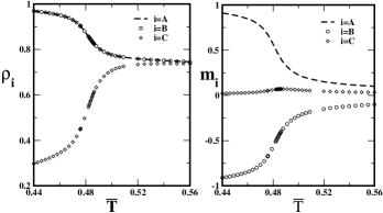
Figure 10: Graph $(a)$ presents the plot of sublattices densities $\rho_{i}$, with $i=A,B,C$ vs reduced temperature $\overline{T}$. In graph $(b)$, we have average particle orientation $m_{i}$ on each sublattice vs $\overline{T}$. In both cases, $\mu=-1.40$ and $\zeta=1/10$.

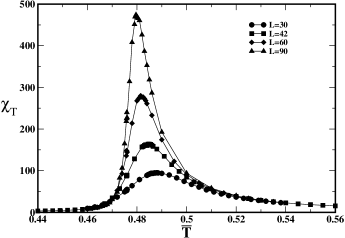
Figure 11: Isothermal susceptibility $\chi_{\scriptscriptstyle{T}}$ vs. reduced temperature $\overline{T}$ for $\zeta=1/10$ and $\overline{\mu}=-1.40$ and different lattice sizes $L$.

In order to check the location of the critical line, the fourth-order cumulant for the order parameter

$$U_{4}=1-\frac{\langle\psi^{4}\rangle}{3\langle\psi^{2}\rangle^{2}}\;,$$ (9)

was computed for different lattice sizes. The results are shown in Fig. 15 for $\zeta=1/10$, $\overline{\mu}=-1.40$ and lattice sizes $L=30,42,60,90$. The crossing of the lines representing different lattice sizes at a single point confirm the presence of criticality. Computed cumulants for other values of the chemical potential display analogous behavior, lending confidence to the interpretation of criticality.

But to what universality class does the critical order-disorder line belong? In order to answer this question we have analyzed the value of the cumulant at the crossing point as well as the order parameter scaling with size.

The cumulant $U_{4}$ displays different regimes at low and high temperatures: for low temperatures, it approaches the value $2/3$, while for high temperatures it approaches $0$. At the phase transition temperature, $\overline{T}_{c}=0.4760(2)$, it displays a non trivial value $0.610(5)$ for all lattice sizes. The non-trivial value of the cumulant $U_{4}\approx 0.610$ at the criticality is characteristic of systems belonging to the Ising universality class.

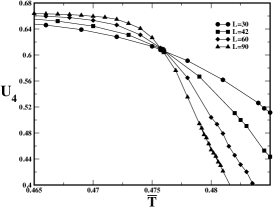
Figure 12: Fourth-order cumulant versus reduced temperature $\overline{T}$ for $\overline{\mu}=-1.40$, $\zeta=1/10$ and different lattice sizes $L$.

Next we examine the scaling of the order parameter. According to the finite size scaling theory Bi92 , at the critical point the order parameter decreases algebraically with the system size through the relation $\psi\sim L^{-\beta/\nu}$, where $\beta/\nu$ is the associated critical exponent. The critical exponent $\nu$ describes the spatial length correlation $\xi$ which diverges at the critical point according to the law $\xi\sim{\bar{t}}^{-\nu}$, where ${\bar{t}}=\overline{T}-\overline{T}_{c}$. For finite systems, it leads to the expression $\overline{T}_{L}-\overline{T}^{\prime\prime}_{c}\sim L^{-1/\nu}$ Bi92 , where $\overline{T}_{L}$ is the pseudo critical temperature, obtained by a maximum in “some susceptibility”. Therefore, log-log plots of $\psi$ and $\overline{T}_{L}-\overline{T}_{\infty}$ vs. $L$ yield the exponents $\beta/\nu$ and $\nu$, respectively. Fig. 13 (a) and (b) illustrate such plots for $\zeta=1/10$ and $\overline{\mu}=-1.40$. From the plots we obtain $\beta/\nu=0.124(3)$ and $\nu=1.03(2)$. These values are in excellent agreement with exact values for the Ising model $\beta=1/8$ and $\nu=1$, thus classifying the order-disorder transition of the BL model in the Ising universality class.

Figure 13: In the graphs $(a)$ and $(b)$ we have a log-log plot of the $\overline{T}^{*}\equiv\overline{T}_{L}-\overline{T}_{\infty}$ and $\psi$ vs. $L$ for $\zeta=1/10$ and $\overline{\mu}=-1.40$. The continuous lines have slope $1.03(2)$ and $0.124(3)$, respectively.

This conclusion is in contrast to the suggestion of Patrykiejew Pa99 and co-workers for the continuous liquid-liquid line. They propose that it would be an example of a second-order phase transition in the Ehrenfest classification, as demonstrated by discontinuity of the specific heat at constant volume $C_{V}$ at the transition. In Fig. 14 we show the dependence of $c_{V}=C_{v}/V$ and $c_{P}=C_{P}/V$ versus the reduced chemical potential $\overline{\mu}$ for $\overline{T}=0.35$. The constant volume and constant pressure specific heats were calculated from simulation data at constant chemical potential through expressions Al87

$$C_{V}=\frac{1}{k_{B}T^{2}}(\langle\delta{\cal H}^{2}\rangle_{\mu VT}-\frac{\langle\delta{\cal H}\delta N\rangle^{2}_{\mu VT}}{\langle\delta N^{2}\rangle_{\mu VT}}),$$ (10)

and

$$C_{P}=C_{V}+TV\alpha_{P}^{2}/{k_{T}},$$ (11)

where $k_{T}=K_{T}/V$, $K_{T}=\frac{V}{N^{2}k_{B}T}\langle\delta N^{2}\rangle_{\mu VT}$ and

$$\alpha_{P}=\frac{PK_{T}}{T}-\frac{\langle\delta{\cal H}\delta N\rangle_{\mu VT}}{Nk_{B}T^{2}}+\frac{\langle{\cal H}\rangle_{\mu VT}\langle\delta N^{2}\rangle_{\mu VT}}{N^{2}k_{B}T^{2}},$$ (12)

where $N=\sum_{i=1}^{V}\eta_{i}$ and $\delta X=X-\langle X\rangle$ with $X={\cal H}$ and $N$. Our results show that the constant volume specific heat $c_{V}$ displays a discontinuity at $\overline{\mu}=-1.98$, close to the gas-liquid transition line (see Fig. 6), and a small peak close to $\overline{\mu}=-1.74$, that increases by increasing $L$, which is in consistency with the transition point in the corresponding phase diagram (Fig. 6) obtained by means of the isothermal susceptibility analysis. In Ref.Pa99 the authors might have been misled by the absence of a phase diagram in the chemical potential vs. temperature plane. The specific heat presented in Ref.Pa99 corresponds to our temperature $\overline{T}=0.175$ footnote . At this temperature, the gas-liquid transition is near $\overline{\mu}=-7.4$, in their units, whereas the liquid-liquid transition is near $\overline{\mu}=-5.7$, in the same units. The discontinuity presented in the paper is near $\overline{\mu}=-7.3$, and thus must correspond to the gas-liquid transition. Ranges below $\overline{\mu}=-6$ are absent from their figure, so the liquid-liquid transition peak is not shown.

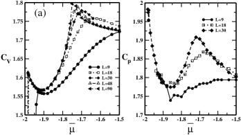
Figure 14: Specific heat at constant volume $c_{V}$ and at constant pressure $c_{P}$ versus $\overline{\mu}$ for $\overline{T}=0.35$ for the BL model and $\zeta=1/4$.

III.4 Anomalous Properties

In this section we present data for the model particle and H-bond densities, and for model entropy.

The presence of a low density liquid suggests that a line of maxima of densities exists. Such maxima were looked for both at constant chemical potential and constant pressure and displayed in the model phase diagrams as TMD lines (see Figs. 3 and 4). Note that the TMD crosses the LDL-HDL critical line in the case of strong bonds ($\zeta=1/10$): the anomaly is inside the LDL phase at low pressures and migrates to the HDL phase at higher pressures. In the case of weaker bonds ($\zeta=1/4$), the anomaly is present only in the HDL phase.

However, as discussed in the previous subsection, correlations between system density and hydrogen-bond density per particle seem to be of some importance. We therefore compare the behavior of the two densities with temperature, for both strong and weak bonds. Figs. 15 (a) and (b) show data for the density $\rho$ vs. $\overline{T}$, for different fixed pressures $P$. For low pressures, the density presents a maximum. In contrast, for higher pressures $P$, the density is a decreasing function of temperature. Particle density behavior is closely accompanied by hydrogen-bond density behavior (Fig. 15 (c) and (d)). For the lower pressures, for which densities present a maximum, hydrogen bond densities decrease with temperature. For the lowest pressure, at which a density maximum is clearly seen, an inflection point of the H-bond density occurs is present at the same temperature. On the other hand, for the higher pressures, for which density is a decreasing function of temperature, hydrogen bond densities increase mildly, at low temperatures. The low pressure behavior coincides with the qualitative picture which has been ascribed to water for a long time: density increases while the hydrogen-bond network distorts, implying a decreasing H-bond density. On the other hand, the increasing H-bond density at higher pressures, low temperatures, suggests that the appearance of empty sites allows for more bonding.

Figure 15: Dependence of the quantities $\rho$, $\rho_{hb}$ and $s$ versus $\overline{T}$ for several values of pressure $p$ for the BL model. The graphs $(a),(c),(e)$ and $(b),(d),(f)$ restrict to the regimes $\zeta=1/10$ and $\zeta=1/4$, respectively.

Finally, entropy per site is shown in Fig. 15 (e) and (f). For the strong bond case, $\zeta=1/10$, the degeneracy of the HDL ground state is clearly seen (for $\overline{P}=0.8$ and $\overline{P}=1.2$). Moreover, the thermodynamic identity $\delta S/\delta P=-\delta V/\delta T$ allows interpretation of entropy behavior as complementary to density behavior (Fig. 15 (a) and (b)). Note the inversion of the relative position of entropies at different pressures, at fixed temperature, before and after the curves cross: at low temperatures, the low pressure curves, which present increasing density as a function of temperature, display lower entropy than the higher pressure entropies, associated with monotonic decreasing density, as function of temperature. At higher temperatures, the situation is opposite: the lower pressure entropies are higher than the higher pressure entropies. Thus the anomalous density behavior is accompanied by an ”anomalous” entropy behavior, in which entropy increases with pressure. Differently from normal liquids, this can be rationalized in terms of disordering of bonds: entropy increases because bond disordering dominates over positional ordering, as density is increased with pressure.

IV Final Comments

We have investigated the Bell-Lavis model for liquid water through numerical simulations in order to shade some light in the role played by the orientational degrees of freedom of this model in the liquid-liquid transition. Our study has allowed the clarification of the nature of the liquid-liquid transition. Previous careful mean-field studies, such as calculations on the Bethe lattice Ba08 or through the cluster variation method Br02 yielded liquid-liquid coexistence with a small density gap. The Monte Carlo simulations demonstrate that the transition is continuous. Moreover, our finite scaling analyses indicate that the transition is in the Ising universality class.

In the absence of a density gap, characterization of the transition requires establishing an order parameter. Inspired on the mapping on the antiferromagnetic spin model, we propose an order parameter based on the difference in sublattice densities, associated to the highly bonded configurations. This order parameter presents a divergent susceptibility at the critical temperature. On the other hand, we have also shown that positional order on sublattices is accompanied by orientational order. Thus the ordered LDL phase presents both positional and orientational order which disappear in the HDL phase.

In the analysis of the thermodynamic variables we were able to accompany number and H-bond densities as well as entropy per particle. The latter is calculated directly from simulations through a transfer matrix representation of the model Hamiltonian. Comparison of the behavior of the three densities with temperature shows that the density anomaly is accompanied by inflection points both in hydrogen bond density as well as in entropy per particle. Such behavior was suggested in the mean-field approach Ba08 , but is made much more clear in the simulation data.

In relation to the density anomaly, it must be pointed out that the line of density maxima (TMD) which was located in the metastable HDL phase for the Bethe lattice, is turned stable through fluctuations present in the Monte Carlo procedure.

As a final remark, we should say that a real liquid-liquid transition would not be continuous transition, since liquid polymorphism is understood do imply discontinuity in density across the transition. Could the transition become first-order in three dimensions? This is a point to be cleared. However, the Bell-Lavis model has no trivial extension to three dimensions. Nonetheless, the feature that makes it an interesting model is the fact that it is an orientational model with attractive van der Waals interactions. This is not the case for every other orientational model in the literature that we know of. Thus it remains to be cleared whether orientational models with attractive isotropic interactions are able to yield liquid-liquid coexistence.

Acknowledgments

C.E.F acknowledges the partial financial support by FAPESP, under grant 06/51286-8 and CNPq.

Appendix A Pressure Calculation

In this appendix the pressure is obtained from the grand potential free energy Sa95 . In order to describe the method briefly, let us consider a triangular lattice with $V$ sites divided in $N$ successive layers $S_{i}\equiv(\eta_{1,i},\eta_{2,i},...,\eta_{N,i})$ with $L$ sites, $V=L\times N$. The Hamiltonian may be decomposed in the following way

$${\cal H}=\sum_{k=1}^{N}{\cal H}(S_{k},S_{k+1}),$$ (13)

where due to the periodic boundary conditions $S_{N+1}=S_{1}$.

The probability $P(S_{1},S_{2},...,S_{N})$ of a given configuration of the system is given by

$$P(S_{1},S_{2},...,S_{N})=\frac{1}{\Xi}T(S_{1},S_{2})T(S_{2},S_{3})...T(S_{N},S_{1}),$$ (14)

where $T(S_{k},S_{k+1})\equiv\exp(-\beta{\cal H}(S_{k},S_{k+1}))$ is an element of the transfer matrix $T$ and

$$\Xi=\rm Tr(\it{T^{N}}),$$ (15)

where $\Xi$ is the Grand-Canonical partition function. By using the spectral expansion of the matrix $T$ it is possible to show Sa95 that

$$\lambda_{0}=\frac{<T(S_{1},S_{1})>}{<\delta_{S_{1},S_{2}}>},$$ (16)

where $\lambda_{0}$ denotes the largest eigenvalue, which is evaluated from averages $<T(S_{1},S_{1})>$ and $<\delta_{S_{1},S_{2}}>$. The quantity $T(S_{1},S_{1})$ is obtained from $T(S_{k},S_{k+1})$ by taking $S_{k}=S_{k+1}$, where

$$T(S_{k},S_{k+1})=\exp\{\sum_{i=1}^{L}[\eta_{i,k}(\eta_{i,k+1}+\eta_{i+1,k}+\eta_{i+1,k+1})$$ (17)

$$(\epsilon_{vdw}+\epsilon_{hb}\tau_{i,k}(\tau_{i,k+1}+\tau_{i+1,k}+\tau_{i+1,k+1})+\mu\eta_{i,k})]\},$$

and $\delta_{S_{1},S_{2}}=1$ when layers $S_{1}$ and $S_{2}$ are equal and zero otherwise. Finally, the free energy is evaluated from the largest eigenvalue through the relation

$$\frac{\Phi}{V}=-\frac{1}{\beta V}\ln\lambda_{0}=-P$$ (18)

where $V$ is the volume (number of sites in the lattice) and $\Phi$ is the grand potential free energy. The entropy per site is evaluated from the grand potential through the formula

$$s=\frac{u-\phi}{T},$$ (19)

where $u=U/V$ and $\phi=\Phi/V$.

References

- (1) M. Chaplin, Sixty-three anomalies of water, http://www.lsbu.ac.uk/water/anmlies.html, 2006.
- (2) C. A. Angell, E. D. Finch, and P. Bach, J. Chem. Phys. 65, 3065 (1976).
- (3) P. H. Poole, F. Sciortino, U. Essmann, and H. E. Stanley, Nature (London) 360, 324 (1992).
- (4) Y. Katayama, T. Mizutani, W. Utsumi, O. Shimomura, M. Yamakata, and K. Funakoshi, Nature (London) 403, 170 (2000).
- (5) G. Monaco, F. S., W. A. Crichton, and M. Mezouar, Phys. Rev. Lett. 90, 255701 (2003).
- (6) D. J. Lacks, Phys. Rev. Lett. 84, 4629 (2000).
- (7) P. T. Cummings and G. Stell, Mol. Phys. 43, 1267 (1981).
- (8) M. Togaya, Phys. Rev. Lett. 79, 2474 (1997).
- (9) A. B. de Oliveira, P. A. Netz, T. Colla, and M. C. Barbosa, J. Chem. Phys. 124, 084505 (2006).
- (10) A. B. de Oliveira, P. A. Netz, T. Colla, and M. C. Barbosa, J. Chem. Phys. 125, 124503 (2006).
- (11) M. C. Wilding and P. F. McMillan, J. Non-Cryst. Solids 293, 357 (2001).
- (12) P. C. Hemmer and G. Stell, Phys. Rev. Lett. 24, 1284 (1970).
- (13) E. A. Jagla, J. Chem. Phys. 110, 451 (1999).
- (14) P. J. Camp, Phys. Rev. E 68, 061506 (2003).
- (15) P. Kumar, S. V. Buldyrev, F. Sciortino, E. Zaccarelli, and H. E. Stanley, Phys. Rev. E 72, 021501 (2005).
- (16) P. A. Netz, S. Buldyrev, M. C. Barbosa, and H. E. Stanley, Physical Review E 73, 061504 (2006).
- (17) A. Balladares and M. C. Barbosa, J. Phys.: Cond. Matter 16, 8811 (2004).
- (18) A. B. de Oliveira and M. C. Barbosa, J. Phys.: Cond. Matter 17, 399 (2005).
- (19) S. Sastry, F. Sciortino, and H. E. Stanley, Journal of Chem. Phys. 98, 9863 (1993).
- (20) S. Sastry, P. G. Debenedetti, F. Sciortino, and H. E. Stanley, Phys. Rev. E 53, 6144 (1996).
- (21) G. Franzese, M. I. Marques, and H. E. Stanley, Phys. Rev. E 67, 011103 (2003).
- (22) A. Patrykiejew, O. Pizio, and S. Sokolowski, Phys. Rev. Lett 83, 3442 (1999).
- (23) C. J. Roberts and P. G. Debenedetti, Journal of Chem. Phys. 105, 658 (1996).
- (24) G. M. Bell and D. A. Lavis, Journal of Phys. A 3, 568 (1970).
- (25) D. A. Lavis, J. Phys. C 6, 1530 (1973).
- (26) A. P. Young and D. A. Lavis, J. Phys. A 12, 229 (1979).
- (27) B. W. Southern and D. A. Lavis, J. Phys. A 13, 251 (1980).
- (28) N. A. M. Besseling and J. Lykema, J. Phys. Chem 98, 11610 (1994).
- (29) V. B. Henriques and M. C. Barbosa, Phys. Rev. E 71, 031504 (2005).
- (30) V. B. Henriques, N. Guisoni, M. A. Barbosa, M. Thielo, and M. C. Barbosa, Mol. Phys. 103, 3001 (2005).
- (31) M. Girardi, A. L. Balladares, V. Henriques, and M. C. Barbosa, Journal of Chem. Phys. 126, 064503 (2007).
- (32) A. L. Balladares, V. Henriques, and M. C. Barbosa, J. Phys.: Condens. Matter 19, 116105 (2007).
- (33) P. P. Bruscolini, A. Pelizzola, and L. Casetti, Phys. Rev. Lett 88, 089601 (2002).
- (34) M. A. A. Barbosa and V. B. Henriques, Phys. Rev. E 77, 051204 (2008).
- (35) K. Binder and D. W. Heermann, Monte Carlo Simulation in Statistical Physics, Springer-Verlag, New York, 1992.
- (36) M. P. Allen and D. J. Tildesley, Computer Simulations of Liquids, Clarendon, Oxford, 1987.
- (37) all their reduced values have a factor , since they have considered reduced unities in terms of the van der Waals energy .
- (38) R. A. Sauerwein and M. J. de Oliveira, Phys. Rev. B 52, 3060 (1995).