The C+N+O abundances and the splitting of the subgiant branch in the Globular Cluster NGC 1851

Abstract

Among the newly discovered features of multiple stellar populations in Globular Clusters, the cluster NGC 1851 harbours a double subgiant branch, that can be explained in terms of two stellar generations, only slightly differing in age, the younger one having an increased total C+N+O abundance. Thanks to this difference in the chemistry, a fit can be made to the subgiant branches, roughly consistent with the C+N+O abundance variations already discovered two decades ago, and confirmed by recent spectroscopic data. We compute theoretical isochrones for the main sequence turnoff, by adopting four chemical mixtures for the opacities and nuclear reaction rates. The standard mixture has Z=10^-3 and [$\alpha$/Fe]=0.4, the others have C+N+O respectively equal to 2, 3 and 5 times the standard mixture, according to the element abundance distribution described in the text. We compare tracks and isochrones, and show how the results depend on the total CNO abundance. We notice that different initial CNO abundances between two clusters, otherwise similar in metallicity and age, may lead to differences in the turnoff morphology that can be easily attributed to an age difference. We simulate the main sequence and subgiant branch data for NGC 1851 and show that an increase of C+N+O by a factor $\sim$3 best reproduces the shift between the subgiant branches. According to spectroscopic data by Yong et al., the C+N+O abundance in this cluster appears correlated with the abundance of s-process elements, Na and Al, and this makes massive AGBs the best progenitors of the C+N+O enriched population. We compare the main sequence width in the color m_F336W-m_F814W with models, and find that the maximum helium abundance compatible with the data is Y$\simeq$0.29. We consider the result in the framework of the formation of the second stellar generation in globular clusters, for the bulk of which we estimate a helium abundance of Y$\lower 2.15277pt\hbox{$\;\buildrel<\over{\sim}\;$}0.26$. The precise value depends on which are the AGB masses from which the C+N+O enriched matter originates, and on the amount of dilution with the pristine gas.

1 Introduction

Figure 1: Variation with temperature of the opacity of the mixtures used in the present investigation. At the top of the figures, the value of R=density/temperature³ and of the hydrogen mass fraction X are labelled. Upper panel: opacity values for the standard (solid track), $\alpha-$ enhanced case, and for the mixtures with CNO abundances increased by a factor 3 (dotted) and 5 (dashed), corresponding to a total metallicity Z=0.00235 and Z=0.00350. For the two latter cases we plot the values for three total metallicities Z=1, 2, and 4$\times 10^{-3}$ (from left to right). Lower panel: opacities in the low-temperature regime, for the mixtures with CNO enhancements of 2 (solid), 3 (dotted), and 5 (dashed).

The observations of Globular Cluster (GC) stars still need to be interpreted in a fully consistent frame. Nevertheless, a general consensus is emerging on the fact that most GCs can not be considered any longer simple stellar populations, and that “self–enrichment” is a common feature among them. The first suspicions originated from the well known “chemical anomalies”, already noted in the seventies (such as the Na–O and Mg–Al anticorrelations). Recently observed to be present at the turnoff (TO) and among the subgiants (e.g. Gratton et al., 2001; Briley et al., 2002, 2004), they must be attributed to some process of self–enrichment occurring at the first stages of the cluster life. A decisive feature indicating the presence of more than one population in GCs has been the observation of multiple, well separated sequences. Multiple main sequences have been found in $\omega$ Cen (Bedin et al., 2004; Piotto et al., 2005) and NGC 2808 (D’Antona et al., 2005; Piotto et al., 2007). Besides, multiple subgiant branches have been observed in NGC 1851 (Milone et al., 2008) and other clusters, among which NGC 6388 (Piotto, 2009). The former phenomenon can only be interpreted in terms of populations with different helium content (D’Antona et al., 2002; Norris, 2004). The latter may be discussed in terms of a difference in age (Milone et al., 2008), or in total CNO abundance (Cassisi et al., 2008), and is the subject of the present work. In both cases, we are left with the difficulty of finding a consistent origin for these populations. We can speculate that there was a first epoch of star formation, that gave origin to the “normal” (first generation, hereinafter FG) stars, with CNO and other abundances similar to Population II field stars of the same metallicity. Afterwards, there must have been some other epoch of star formation (second generation, hereinafter SG), including material heavily processed through the hot CNO cycle in the progenitors, belonging to the FG, but not enriched in the heavy elements expected in supernova ejecta. This material either comes entirely from the stars belonging to the first stellar generation, or it is a mixture of processed gas and pristine matter of the initial star forming cloud.

The SG in most clusters is a high fraction of the total number of stars (Carretta et al., 2008; D’Antona & Caloi, 2008). In order to have enough CNO processed material available, it is necessary that “self–enrichment” is a result of pollution from an initial stellar population much larger than the stellar content of today’s GCs. This is generally attributed either to the dynamic loss of a great fraction of the clusters’ FG stars in the early evolutionary phases (D’Ercole et al., 2008), or to the formation of the GC within a much larger stellar environment, such as a dwarf galaxy, where the polluting matter is supplied by the surrounding stars (Bekki & Norris, 2006).

One of the important constraints for the progenitors was usually considered to be that their matter must have been processed through the hot CNO cycle, and not, or only marginally, through the helium burning phases, since the sum of CNO elements is the same within observational errors in the “normal” and in the anomalous stars (Cohen & Meléndez, 2005; Ivans et al., 1999). If the polluting matter is identified with the envelopes of asymptotic giant branch (AGB) stars (Ventura et al., 2001, 2002), these AGBs must be very massive, so that their evolution is only scarcely affected by the third dredge up, that acts to increase the surface abundance of the primary carbon formed in the helium intershell during the thermal pulses, and then partially mixed into the external envelope (e.g. Iben & Renzini, 1983). Otherwhise, pollution must come from a totally different kind of objects, such as the envelopes of fast rotating massive stars during the core H–burning phase (Meynet et al., 2006; Decressin et al., 2007), and in this case we do not expect any C+N+O enhancement at all, as mentioned before.

Recently, the constancy of C+N+O has been challenged by the discovery that the cluster NGC 1851 displays a double subgiant branch (SGB) (Milone et al., 2008). No such splitting is present in the main sequence of NGC 1851, indicating a normal —or close to normal (see Sect.4)— helium content for both SGBs. This has been interpreted by Milone et al. (2008) as due to a $\sim$1Gyr age difference between the two SGB populations. This age difference is much larger than generally believed possible for a GC (e.g. D’Ercole et al., 2008). An alternative interpretation has been given by Cassisi et al. (2008): they were able to reproduce the splitting by assuming that stars in the faint SGB (fSGB) have a larger C+N+O abundance and similar age of the bright SGB (bSGB). At the same time, Yong & Grundahl (2008) have shown that this cluster harbors a star-to-star abundance variation in the s-process elements Zr and La and that the abundances of these elements were correlated with the abundances of Na and Al, and anticorrelated with O. Furthermore, within the small sample of 8 giants examined, there was a hint that the abundances of the s-process elements is bimodal. Most recently, Yong et al. (2009) have determined the C, N, and O abundances in four red giants, selected to span the range of Na, Al and s–process abundances, and found that indeed the sum of C+N+O exhibits a range of 0.6dex, a factor 4, and that the light elements abundances, s–process and total C+N+O abundances are correlated. These observations support indeed the AGB stars as progenitors of the stars populating the fSGB in NGC 1851, as suggested by Cassisi et al. (2008). Signs of a milder C+N+O enrichment in other clusters have been noticed by Carretta et al. (2005) in NGC 6397 and NGC 6752, but NGC 1851 is to date the most prominent example (see Piotto, 2009, for further examples). As we have noticed, in most GCs the (possible) AGB progenitors of the SG must be so massive that the chemistry of the ejecta is scarcely affected by the third dredge up, with only a minor increase in the total C+N+O abundance. But the effects of the third dredge up increase with time: its efficiency increases when the evolving mass decreases (e.g. Ventura & D’Antona, 2008, Table 1). So the observability of a C+N+O increase depends on how long the phase of star formation of the SG stars lasts. Yong et al. (2009) propose that in NGC 1851 this phase lasts long enough that the effect of the third dredge up is evident.

In this work, we consider the evolution of low mass stars evolving at GC ages, with the metallicity of NGC 1851, but considering the effect of an increased C+N+O abundance on the evolution. Cassisi et al. (2008) limited the analysis to a chemistry in which the C+N+O content was approximately doubled with respect to the standard composition, while we consider C+N+O abundances increased by factors 2, 3 and 5. Selection of the individual abundances for C, N and O is explained in Section 2. Inclusion of their effect is considered both in the low temperature and high temperature opacities and in the nuclear reaction network. In Section 3 we present the results, and discuss the time evolution of selected evolutionary tracks, the total mass lost along the RGB, and the relative location of the isochrones in the color magnitude diagram (CMD). In Section 4 we present simulations, in the CMD, of the main sequence and SGB for NGC 1851, under several hypotheses concerning the different compositions necessary to explain the separate SGBs. In Section 5 we discuss the results.

2 Input physics and model computation

All the evolutions presented in this work have been calculated by means of the ATON code for stellar evolution, with the numerical structure described in details in Ventura et al. (1998). Tables of the equation of state are generated in the (gas) pressure-temperature plane, according to the OPAL EOS of the Livermore group (see OPAL webpage, last update in February 2006, Rogers et al., 1996), replaced in the pressure ionization regime by the EOS by Saumon, Chabrier & Van Horn (1995), and extended to the high-density, high-temperature domain according to the treatment by Stoltzmann & Blöcker (2000).

2.1 Standard and non–standard opacities

For the “standard” models we adopt the latest opacities by Ferguson et al. (2005) at temperatures lower than 10000 K and the OPAL opacities in the version documented by Iglesias & Rogers (1996). The mixture adopted is alpha-enhanced, with $[\alpha$/Fe$]=0.4$ (Grevesse & Sauval 1998). Electron conduction opacities were taken from the WEB site of Potekhin (see the web page http://www.ioffe.rssi.ru/astro/conduct/ dated 2006) and correspond to the Potekhin et al. (1999) treatment. The electron opacities are harmonically added to the radiative opacities. For this project we select three different mixtures of elements, having the C, N and O abundances varied with respect to the standard mixture. For the abundances of C, N and O we adopt the values in Table 2 in Ventura & D’Antona (2008), corresponding to the yields of the models with 5, 4.5 and 4$\,{M}_{\odot}$ and metallicity Z=10^-3. These abundances are reported in Table 1. As we see, in the 5$\,{M}_{\odot}$ ejecta Oxygen is depleted by 0.46 dex (the original [O/Fe] is +0.4 in the standard mixture), Carbon is enhanced by 0.13 dex and Nitrogen is enhanced by 1.7 dex. The total C+N+O is a factor 2.1 larger than in the standard mixture. The 4.5$\,{M}_{\odot}$ total CNO content is 3.1 times the standard one, and the 4$\,{M}_{\odot}$ one is a factor 4.9 larger. We remarked that the 4 red giants of NGC 1851 examined by Yong et al. (2009) show a maximum variation of $\sim$4 in C+N+O. Individually, carbon and oxygen vary up to about a factor 3 and nitrogen by a factor 7. With our present choices, we are then enhancing the nitrogen increase with respect to these few observational data. More observations and new models may be useful in future analyses. The total ”metallicity” Z in mass fraction for the three CNO–enhanced mixtures is listed in Table 1.

Table 1: Chemistry of the models

Name	Z	total CNO	[C/Fe]	[N/Fe]	[O/Fe]	Y	M/M⊙(AGB)	age (Myr)
CNOx1 (standard)	0.00100	1	0.00	0.00	0.40	0.240	-	-
CNOx2	0.00185	2.1	0.13	1.70	-0.06	0.324	5.0	103
CNOx3	0.00235	3.1	0.12	1.89	0.19	0.310	4.5	128
CNOx5	0.00350	4.9	0.14	2.02	0.44	0.281	4.0	166

The radiative opacities for these CNO enhanced mixtures have been computed on purpose for this work. For temperatures above 10000 K we utilized the online computations from the OPAL group found at http://physci.llnl.gov/Research/OPAL/opal.html; for lower temperatures we computed opacities with the Ferguson et al. (2005) code for the Z mixtures listed in table 1. Figure 1 shows the differences among the opacities of the various mixtures in the high– and low–temperature regime. In the upper panel we see that the largest differences are found in the ioniziation region of the CNO elements, around $\log T\sim 6$. The lower panel of Fig. 1 shows the low temperature opacities for the three enhanced computations. Above $\log T\sim$3.5 few differences are noted as the opacity is dominated by hydrogen. However, at lower temperatures the opacity significantly deviates for each run from the standard. This deviation is due to more and more O available (due to the CNO enhancements) for the formation of molecular water at these temperatures. The low temperature opacities do not affect the structure of the models we are considering, while at the larger temperatures of the stellar interiors some differences appear. In addition, the CNO total abundance affects the time evolution as soon as the stars begin evolving at the turnoff, where the CN cycle becomes important.

2.2 Color –T_eff conversions

Our aim is to compare the theoretical predictions with the data by Milone et al. (2008) for NGC 1851, obtained in the HST Advanced Camera for Surveys (ACS) filters F814W and F606W. Therefore we convert our L,T_eff values into these magnitudes by using the transformations for ACS bands by Bedin et al. (2005), based on the solar scaled models by Cassisi et al. (2004). We note that the $\alpha$–enhanced versus solar–scaled transformations, for the metallicity and colors we are using, do not differ for T_eff$\;\buildrel>\over{\sim}\;$5000K. On the other hand, we are also dealing with CNO enhanced mixtures, and in principle the use of the same transformations could not be adequate. However, we refer to Pietrinferni et al. (2009), who widely discuss this issue, and conclude that, in broadband filters not bluer than the Johnson V band, the effect of this inconsistency should be very small, since at least the color - T_eff transformations are largely independent on the metals and their distribution (see Alonso et al., 1996, 1999; Cassisi et al., 2004). This statement luckily applies to our case, as we are dealing with red and near infrared bands. Possible differences in the conversions due to the enhanced CNO may of course change the quantitative conclusions of our analysis, so that we raise the problem of the computation of proper color–T_eff conversions for CNO enhanced mixtures.

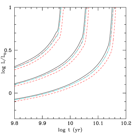
Figure 2: Luminosity versus time evolution for the masses 0.8, 0.85 and 0.9$\,{M}_{\odot}$(from right to left) as a function of the CNO enhancement. The full (black) lines are the CNOx1 evolution. The CNOx2, CNOx3 and CNOx5 tracks are located progressively at smaller luminosity.

Figure 3: Comparison between the HR diagram of the standard CNOx1 track of 0.85$\,{M}_{\odot}$(full line) and of the CNOx3 track (dotted line), with the evolution of the same mass, obtained by assuming the opacities of the standard track, but the CNO abundances of the CNOx3 track (dashed line).

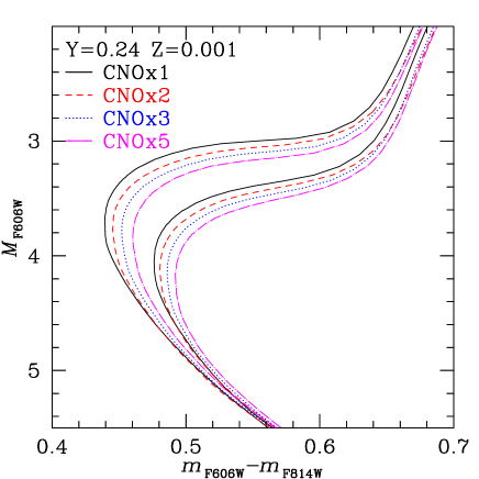
Figure 4: Isochrones in the plane $M_{\rm F606W}$ vs. the color $M_{\rm F606W}-M_{\rm F814W}$. The top group of lines refers to an age of 9Gyr, the lower set are for an age of 13Gyr. The isochrone luminosity decreases as a function of the CNO enhancement.

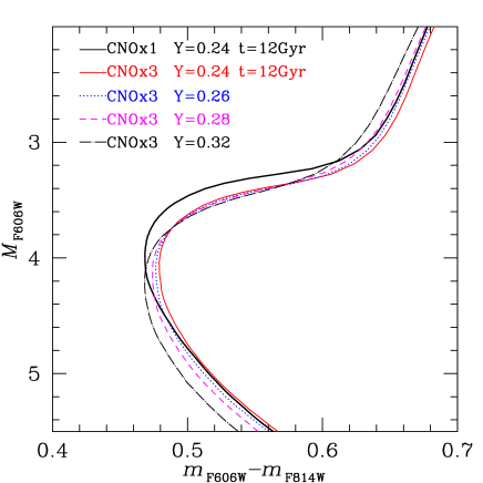
Figure 5: Isochrones in the plane $M_{\rm F606W}$ vs. $m_{\rm F606W}-m_{\rm F814W}$. The standard Y=0.24 CNOx1 t=12Gyr isochrone is the upper line. The lower lines are for the same age and different helium content. The SGB luminosity is only slightly altered for Y=0.32.

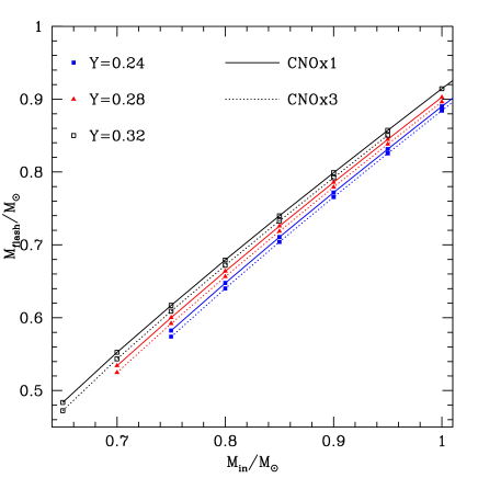
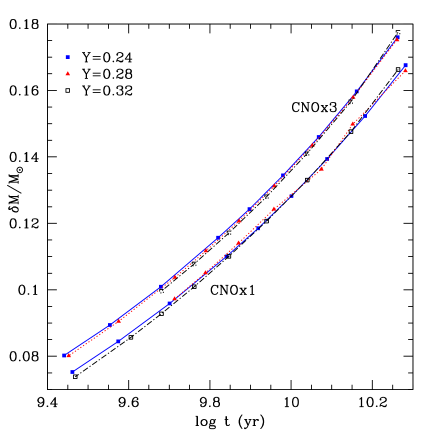
Figure 6: The top panel shows the mass at the helium flash, M_flash as a function of the total stellar mass, for the three labelled helium contents and for the standard tracks. The dotted lines show the same for the CNOx3 tracks. Although for a fixed mass there is a dependence of M_flash on Y and CNO, the bottom panel shows that the mass lost along the RGB ($\delta$M) practically does not depend on the helium content at a fixed epoch. On the contrary, at a given age, $\delta$M is $\sim 0.01$$\,{M}_{\odot}$ larger for the CNO enhanced isochrones. We plot in the figure only the CNOx1 and the CNOx3 cases, the other two cases are practically superimposed to the CNOx3 lines.

2.3 Synthetic CMD Simulations

For a better comparison of the models with the data, we use simulations for the main sequence and subgiant branch(es). These are obtained by extracting random each star location along a specified isochrone, according to a choice of the initial mass function (IMF). We assume a power law IMF with exponent –1.5 (where Salpeter’s is –2.3). The exact choice of the IMF is inconsequential, as the comparison of the SGBs involves a very small mass interval (see Sect. 4). Gaussian errors consistent with the observational errors on colors and magnitudes close to the turnoff are attached to each extraction. For the double stellar population of NGC 1851, we use a standard isochrone of CNOx1 for 55% of the sample, while the rest is extracted from the isochrone having the same age and enhanced CNO. These percentages are based on the observational analysis by Milone et al. (2009), and are confirmed in the analysis of the subgiant branches made in Sect. 4, describing the comparison between the simulations and data.

3 Model results

3.1 The isochrone location: dating GCs with the same metallicity and different CNO

Figure 2 shows the luminosity versus time evolution of masses 0.8, 0.85 and 0.9$\,{M}_{\odot}$ for different CNO enhancement. The CNOx1 standard tracks have the fastest evolution, because the CNO enhanced tracks lie at progressively lower main sequence luminosity. In order to understand better the different roles of the opacities and nuclear reaction rates, we show in Figure 3 the HR diagram location of a track of 0.85$\,{M}_{\odot}$, having the standard CNOx1 opacities, but CNOx3 abundances (in particular the CNOx3 abundances are used in the nuclear network). We see that the main sequence evolution is quite similar to that of the standard CNOx1 track, as burning occurs mainly through the proton–proton chain. The main sequence of the track is just slightly more luminous than for the standard CNOx1 track, and the evolutionary times are consequently barely shorter. The turnoff, however, occurs at a smaller luminosity, as in that case the CNO cycle dominates. Therefore, the lowering of the turnoff luminosity is mainly due to the effect of the abundances on the final phases main sequence burning, while the lenghtening of the evolutionary times is mainly due to the smaller main sequence luminosity of the models with enhanced CNO.

Globally, the isochrones show a monotonic shift in luminosity and color with increasing CNO. Figure 4 shows that the subgiant location for the same age is fainter for higher CNO, so that these models can in principle reproduce the splitting of the SGBs in NGC 1851, if the two sequences have different CNO content. Figure 5 shows the comparison between the standard SGB for Y=0.24 and the SGBs of the models CNOx3 with different helium contents (Y=0.24, 0.26, 0.28 and 0.32). We see that the SGB shift does not depend on the helium content, at least for this metallicity, while the main sequence location and the red giants become bluer when Y increases (see also Sect. 5).

Considering Fig. 4, we observe that any age determination for a GC can not ignore what is the total C+N+O abundance in its stars. While this is a well known theoretical aspect of evolution (e.g. Simoda & Iben, 1970; Bazzano et al., 1982), it is worth recalling it in this context, now that we have interesting evidence of its possible role. In fact, the interpretation of NGC 1851 data shows this (Cassisi et al., 2008), and we also have other cases where it may be of relevance (Piotto, 2009). The total CNO abundance in the giants of M4 (NGC 6121) is larger than the total CNO of those stars, in NGC 1851, that can be considered “normal” for what concerns the abundances of CNO, s-process elements, Na and Al (see Figure 3 in Yong et al., 2009). Therefore, should we compare these two clusters, their relative age determination should include the dependence on the CNO abundance. In this context, it is worth recalling the large spread in N abundance in all the clusters surveyed (Grundahl et al., 1999), together with the dichotomy between CN strong and CN weak stars in so many GCs. The giants in NGC 6752 present a star-to-star abundance variation in N of 1.95dex (Yong et al., 2008), and a similar spread is present also in the main sequence (Pasquini et al., 2008; Carretta et al., 2005). Variations in C abundance may compensate, but some spread in luminosity at the turn-off of this cluster should be present (Bazzano et al., 1982).

3.2 The mass lost along the red giant branch

All models are evolved by assuming a mass loss rate following Reimers’ (1977) prescription $\dot{M}_{R}=4\cdot 10^{-13}\eta_{R}{LT\over M}$ where the parameter $\eta_{R}$ has been fixed to 0.3 for all the computations. This allows us to find the dependence of the mass lost in the giant phase on the helium and CNO content of the tracks. Of course the results are of some significance only if Reimers’ rate is actually a good description of the mass loss. In a relative sense, the results may be similar for other mass loss rates, if they depend explicitly only on the stellar parameters luminosity and gravity, and do not depend, e.g., on the CNO content. Some results are shown in Fig. 6. In the top panel we see that mass at the helium flash, for a fixed initial mass, increases with Y and decreases with the CNO enhancement. We plot the CNOx1 and CNOx3 case, but the results for the other CNO rich models are similar. However, what matters is the mass lost at fixed age, shown in the bottom panel of Fig. 6. This actually does not depend at all on Y (see also D’Antona & Caloi, 2008), while, for a fixed age, all the CNO enhanced models predict $\sim$0.01$\,{M}_{\odot}$ more mass loss, as shown for the case of the CNOx3 models. These indications are important to predict the horizontal branch (HB) location of stars with different CNO and/or helium content. Cassisi et al. (2008) have shown that the T_eff location of HB models is affected by their enhanced CNO, due to the different relative efficiency of the shell–hydrogen– and core–helium– burning (see their Figure 1, but see also Castellani & Tornambe (1977)).

4 Comparisons

Figure 7 shows the HR diagram of NGC 1851 based on 5 images of 350s in F606W and 5 images of 350s in F814W from the ACS survey by Anderson et al. (2008). Thes exposure are saturated at the basis of the RGB, so the photometry of the RGB comes from two low exposure images (one 20s image in F606W and one 20s image in F814W) and has larger errors. The data in Fig.7 are compared with the isochrones. Distance and reddening are chosen to fit isochrones of ages respectively 9 and 12Gyr in the two panels.

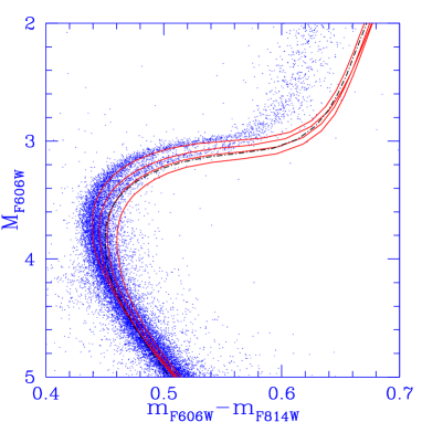
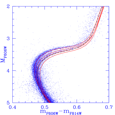
Figure 7: Comparison of isochrones of ages 9 Gyr (top panel) and 12 Gyr (bottom panel) with the HR diagram of NGC 1851. We apply to the data a distance modulus and dereddening in order to fit the “standard” top isochrone to the bSGB. The dashed line (black) is the CNOx3 isochrone of Y=0.26. Distance moduli and reddenings respectively: ($m_{\rm F606W}$–$M_{\rm F606W}$)= 15.72, $\delta$color=0.05mag for the top panel (9Gyr isochrones) and 15.44mag, 0.02mag for the bottom panel (12Gyr isochrones). The continuous (red) lines, starting from the top to the bottom one, are the isochrones for Y=0.24 and respctively CNOx1, CNOx2, CNOx3 and CNOx5.

We see that the giant branch location agrees better with the 12Gyr isochrones, but it is difficult to attribute to this feature a predictive value for the age, as the giant branch location depends on the adopted convection model.

This comparison immediately shows that the fSGB in the cluster lies in between the isochrones corresponding to CNOx2 and CNOx3. This finding is strengthened when we make use of the simulations built up as described in Sect. 2.3. Figure 8 compares the observed HR diagram with simulations for an age of 12 Gyr. The bSGB is reproduced with a standard CNOx1 population, while the fSGB is reproduced assuming a second population with CNOx2 (top), CNOx3 (middle) and CNOx5 (bottom panel).

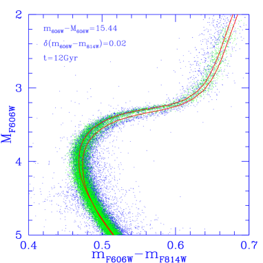
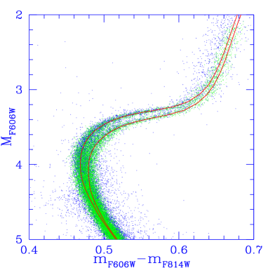
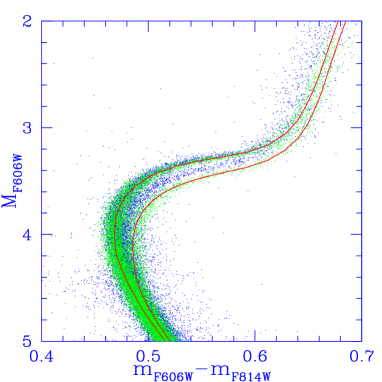
Figure 8: Comparison of NGC 1851 data (blue dots) with simulations (green) for an age of 12 Gyr. Distance modulus and assumed reddening are labelled. The bSGB is simulated with a population having normal (CNOx1) CNO, the fSGB corresponds to a population with CNOx2 (top), CNOx3 (middle) and CNOx5 (bottom panel). The corresponding isochrones of 12 Gyr are also shown. The helium abundance is assumed to be Y=0.24 for both populations.

It is evident, looking at the bottom panel of Fig. 8, that the CNOx5 isochrones are not adequate to describe the splitting of the SGBs: such a CNO enhancement would produce a splitting much larger than observed. The CNOx2 isochrones produce a very small splitting, the CNOx3 isochrones are the closest to the observations.

For a quantitative comparison of observed and simulated HR diagrams we go through a procedure already used by Milone et al. (2009). Fig. 9 illustrates this three-step procedure for the observed ACS/WFC data. We selected by hand two points on the fSGB ($P_{1,f}$,$P_{2,f}$) and two points on the bSGB ($P_{1,b}$,$P_{2,B}$) with the aim of delimiting the SGB region where the split is most evident. These points define the two lines in panel (a), and only stars contained in the region between these lines were used in the following analysis. In panel (b) we have transformed the CMD linearly into a reference frame where: the origin corresponds to $P_{1,b}$; $P_{1,f}$ has unit abscissa, and both $P_{2,b}$ and $P_{2,f}$ have unit ordinate. For convenience, in the following, we indicate as ‘abscissa’ and ‘ordinate’ the abscissa and the ordinate of this reference frame. The dashed green line is the fiducial of the bSGB. We drew it by marking several points on the bSGB, and interpolating a line through them by means of a spline fit. In panel (c) we have calculated the difference between the ‘abscissa’ of each star and the ‘abscissa’ of the fiducial line ($\Delta$ ‘abscissa’).

The histograms in Fig. 10 are the normalized distributions in $\Delta$ ‘abscissa’ for stars in four $\Delta$ ‘ordinate’ intervals. In the three panels of this figure we compare the distribution of the observed data (grey histograms) and the simulations (black histograms). The bSGB corresponds to the population with normal CNO, the fainter SGB corresponds to the CNO $\times$ 2 (left), CNO $\times$ 3 (middle), and CNO $\times$ 5 (right).

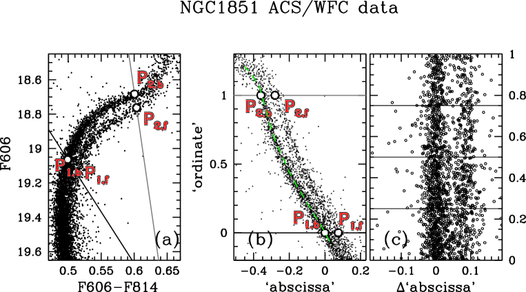
Figure 9: This figure illustrates the procedure for the comparison of the observed data and the simulation. Panel (a) is a zoom of the observed ACS/WFC HR diagram. The two lines delimit the portion of the HR diagram where the split is most evident. Only stars from this region are used to measure the population ratio. In Panel (b) we have linearly transformed the reference frame of Panel (a). The green dashed line is the fiducial of the region around the bSGB. In Panel (c) we plotted stars between the two lines but after the subtraction of the ‘abscissa’.

Figure 10: The histograms show the $\Delta$‘abscissa’ distribution for stars in four $\Delta$‘ordinate’ bins. We compare the distribution of the observed data (grey histograms) and the simulations (black histograms).

If we use slightly helium enriched isochrones (up to Y$\sim$0.28) for the simulation of the fSGB, the results do not change for what concerns the SGB splitting (see Fig. 4). Notice however that the HB observations pose a constraint on the maximum helium abundance of the SG in this cluster: Salaris et al. (2008) were not able to reproduce the HB morphology attributing to the whole blue HB side (probably corresponding to the same population of the fSGB) with models having helium content as high as Y=0.28 (and for larger Y the situation is worse). From the width of the MS, however, we can derive an independent upper limit to the helium abundance of the SG stars, by comparing it with models having different Y.

Figure 11 shows such a comparison for eight magnitude bins of the MS in the color ${\it m}_{\rm F336W}-{\it m}_{\rm F814W}$. From the mean of the eight Y extimates, we derive an upper limit for the He spread in NGC 1851. We find $\Delta Y$=$0.043\pm 0.003$. If the FG has Y=0.24, the maximum possible helium abundance value is Y=0.290$\pm 0.003$.

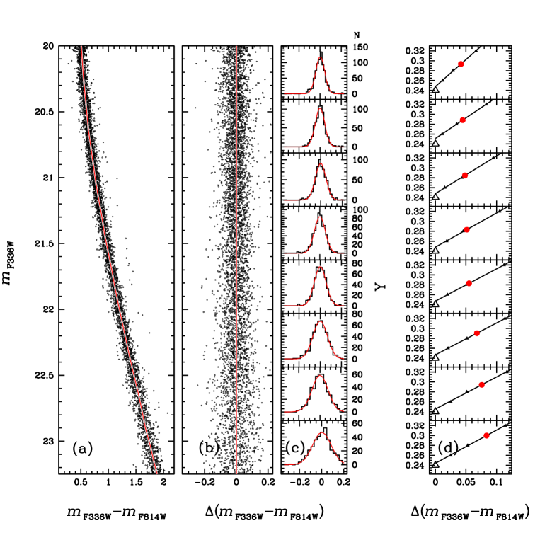
Figure 11: Panel $a$ shows the ${\it m}_{\rm F336W}$ vs. ${\it m}_{\rm F336W}-{\it m}_{\rm F814W}$ CMD already presented in Milone et al.  (2008) with the fiducial line overimposed. Panel $b$ shows the same CMD, after subtracting from each star the color of the fiducial line appropriate for its ${\it m}_{\rm F336W}$ magnitude. The histograms of the color distribution in eight magnitude bins are plotted in panel $c$. In panel $d$ we show the helium content Y as a function of the color distribution in each bin. The three black triangles indicate the MS spread predicted by teoretical models for a SG with CNOx3 and Y=0.26, 0.28, and 0.32, and are used to derive the straight line by means of a least squares fit. The open triangles corresponds to the case where the SG has CNOx1 and Y=0.24. Red circles indicate the Y value corresponding to the observed MS color spread.

5 Discussion

The computed models and the comparison with the data show that the CNO ehnancement required to explain the double SGB in NGC 1851 is of about a factor three. This confirms and puts on a more quantitative basis Cassisi et al. (2008) results. (In the following discussion, anyway, keep in mind that the quantitative conclusions of our analysis are based on the use of the same color–T_eff relations both for CNO normal and CNO enhanced mixtures). So, in this cluster, we need CNO enhancement to fit the HR diagram features. If we add the spectroscopic information from Yong & Grundahl (2008) and Yong et al. (2009), on the presence of s–process enhancement and of a global CNO spread among the cluster giants, we may conclude that massive AGB pollutors are the only reasonable candidates to form the SG stars in the fSGB in NGC 1851.

It is possible to better quantify this statement by looking at Table 1. We choose our compositions, for the elemental abundances and opacity computation, from the pure ejecta of our AGB models of Z=10^-3 (Ventura & D’Antona, 2008). In the table we see that a factor three in CNO is reached in the matter expelled by the 4.5$\,{M}_{\odot}$ stars. If, however, the matter forming the SG stars comes from pure ejecta only, these stars should have a helium content of Y$\sim$0.31. Indeed such a large helium content is to be excluded, based 1) on the main sequence, as it does not show the width required by such a large Y spread (see, Figure 5 and the discussion in Sect. 4); and 2) on the HB morphology, both because the HB lacks very hot stars, and because the blue side of the RR Lyr region is not particularly overluminous (e.g. Salaris et al., 2008).

A possible solution is that the AGB ejecta have been diluted with pristine matter while forming the SG stars. If, e.g., the matter comes preferentially from the 4$\,{M}_{\odot}$, the ejecta would have 5 times the standard CNO, as listed in Table 1. Dilution with 50% of pristine matter gives the required CNO enhancement by a factor 3. In this case, the starting helium abundance in the ejecta was Y=0.28. Diluting it with 50% of matter at Y=0.24, the helium content of the SG stars have Y=0.26, a value not in contradiction with what required by the HB morphology.

It remains to be understood why the SG took such a long time to be formed (according to Table 1, 166Myr is the age at which the 4$\,{M}_{\odot}$ has evolved and ejected its CNO enriched matter into the cluster), while in most other clusters it seems to be formed much earlier, within at most 100 Myr. In fact, Table 1 shows that the masses contributing to the SG must be larger than $\sim$5$\,{M}_{\odot}$, if the total CNO content has to be kept within a factor two of the FG value (Cohen & Meléndez, 2005; Ivans et al., 1999). In addition, the very high helium subpopulations found in a few very massive clusters (Piotto, 2009) require that, in these clusters, part of the SG has been formed by the ejecta of the most massive super–AGB stars (Pumo et al., 2008; D’Ercole et al., 2008), evolving at ages $\sim 30-40$Myr.

The necessity of a C+N+O enhancement in the SG of NGC 1851 is further established with our analysis, following the Cassisi et al. (2008) discussion, and has at least an initial observational basis in the Yong et al. (2009) data. The above detailed formation scenario for this cluster, however, relies on the yields from the models by Ventura & D’Antona (2008) that have been employed in this discussion. Different models, e.g. the set by Karakas & Lattanzio (2007), provide stronger effect of the third dredge up at larger initial masses, mainly because these models adopt of a less efficient convection description (see the discussion in Ventura & D’Antona, 2005a). The Karakas & Lattanzio (2007) yields do not favour the AGB interpretation of observational data for most clusters, namely the quasi–constancy of C+N+O and the shape of the anticorrelation O–Na (Fenner et al., 2004). A possible escape is that the whole range of pollutor masses for the SG is shifted to the super–AGB range, but, to our knowledge, no such models are available by now. However, yields close to those by Karakas & Lattanzio (2007) would change our conclusions on the timescale of formation of an SG, just because the stronger effect of the third dredge up —limited, anyway, to a factor $\sim$3 increase in C+N+O— would be obtained at larger evolving masses ($\sim 6$$\,{M}_{\odot}$) and much shorter evolutionary times.

6 Conclusions

We computed the evolution of standard $\alpha$–enhanced low mass stellar models of metallicity Z=10^-3, and of models with the same [Fe/H], in which the total CNO abundance is larger by factors 2, 3 and 5, according to the elemental distribution expected from the intermediate mass AGB ejecta that can be progenitors of SG stars in Globular Clusters. Our aim is to derive quantitative information about the C+N+O difference required to explain the splitting of the subgiant branch in the GC NGC 1851. Comparison of the models with the data quantifies the necessity of C+N+O enhancement in the fSGB. The amount of total CNO required is a factor of about three larger than the total CNO adopted for the bSGB. We incidentally warn that a difference in total CNO between clusters having the same metallicity may simulate a non negligible age difference. We try to interpret the data on the basis of the massive AGB scenario for the formation of the fSGB, showing the presence of an SG. The ejecta of the AGBs that formed the SG must have a total CNO abundance increased by a factor three at least. Though, if these pure ejecta have formed the SG, its helium abundance would be as high as Y=0.31, incompatible with both the MS color width and the morphology of the HB. We propose that the CNO enrichment in the ejecta was a factor at least 5 larger than the initial CNO, and that the ejecta have been diluted with pristine gas by 50%. In this case, the abundance of helium in the SG comes down to a much more reasonable value of Y=0.26 or less, but we must explain why the SG formation was delayed to a total age of more than 150Myr in this cluster and not in others. Finally, we remember that the quantitative conclusions of our analysis are based on the use of the same color–T_eff relations both for CNO normal and CNO enhanced mixtures. Although this seems reasonable for the red bands we are using (Pietrinferni et al., 2009), the possibility that appropriate color–T_eff relations, when available, may modify the CNO enahncement required to fit the two SGBs in this cluster must be kept in mind.

7 Acknowledgments

This work has been supported through PRIN MIUR 2007 “Multiple stellar populations in globular clusters: census, characterization and origin”. We thank S. Cassisi for useful comments. We also warmly thank the anonymous referee for his careful reading of the first version of the manuscript, and for forcing us to clarify a number of important points.

References

- Alonso et al. (1996) Alonso, A., Arribas, S., & Martinez-Roger, C. 1996, A&A, 313, 873
- Alonso et al. (1999) Alonso, A., Arribas, S., & Martínez-Roger, C. 1999, A&AS, 140, 261
- Anderson et al. (2008) Anderson, J., et al. 2008, AJ, 135, 2055
- Bazzano et al. (1982) Bazzano, A., Caputo, F., Sestili, M., & Castellani, V. 1982, A&A, 111, 312
- Bedin et al. (2004) Bedin, L. R., Piotto, G., Anderson, J., Cassisi, S., King, I. R., Momany, Y., & Carraro, G. 2004, ApJ Letters, 605, L125
- Bedin et al. (2005) Bedin, L. R., Cassisi, S., Castelli, F., Piotto, G., Anderson, J., Salaris, M., Momany, Y., & Pietrinferni, A. 2005, MNRAS, 357, 1038
- Bekki & Norris (2006) Bekki, K., & Norris, J. E. 2006, ApJ Letters, 637, L109
- Briley et al. (2002) Briley, M., Cohen, J. G., & Stetson, P. B. 2002, ApJ, 579, L17
- Briley et al. (2004) Briley, M. M., Harbeck, D., Smith, G. H., & Grebel, E. K. 2004, AJ, 127, 1588
- Carretta et al. (2005) Carretta, E., Gratton, R. G., Lucatello, S., Bragaglia, A., & Bonifacio, P. 2005, A&A, 433, 597
- Carretta et al. (2008) Carretta, E., Bragaglia, A., Gratton, R. G., & Lucatello, S. 2008, arXiv:0811.3591
- Cassisi et al. (2004) Cassisi, S., Salaris, M., Castelli, F., & Pietrinferni, A. 2004, ApJ, 616, 498
- Cassisi et al. (2008) Cassisi, S., Salaris, M., Pietrinferni, A., Piotto, G., Milone, A. P., Bedin, L. R., & Anderson, J. 2008, ApJ, 672, L115
- Castellani & Tornambe (1977) Castellani, V., & Tornambe, A. 1977, A&A, 61, 427
- Cohen & Meléndez (2005) Cohen, J. G., & Meléndez, J. 2005, AJ, 129, 303
- D’Antona et al. (2002) D’Antona, F., Caloi, V., Montalbán, J., Ventura, P., & Gratton, R. 2002, A&A, 395, 69
- D’Antona et al. (2005) D’Antona, F., Bellazzini, M., Caloi, V., Fusi Pecci, F., Galleti, S., & Rood, R. T. 2005, ApJ, 631, 868
- D’Antona & Caloi (2008) D’Antona, F., & Caloi, V. 2008, MNRAS, 390, 693
- Decressin et al. (2007) Decressin, T., Meynet, G., Charbonnel, C., Prantzos, N., & Ekström, S. 2007, A&A, 464, 1029
- D’Ercole et al. (2008) D’Ercole, A., Vesperini, E., D’Antona, F., McMillan, S. L. W., & Recchi, S. 2008, MNRAS, 391, 825
- Fenner et al. (2004) Fenner,Y., Campbell, S., Karakas, A.I., Lattanzio, J.C. & Gibson, B.K. 2004, MNRAS, 353, 789
- Ferguson et al. (2005) Ferguson J. W., Alexander D. R., Allard F. et al., 2005, ApJ, 623, 585
- Gratton et al. (2001) Gratton, R. G., Bonifacio, P., Bragaglia, A., et al. 2001, A&A, 369, 87
- Grevesse & Sauval (1998) Grevesse, N., & Sauval, A.J. 1998, SSRv, 85, 161
- Grundahl et al. (1999) Grundahl, F., Catelan, M., Landsman, W. B., Stetson, P. B., & Andersen, M. I. 1999, ApJ, 524, 242
- Iben & Renzini (1983) Iben, I., Jr., & Renzini, A. 1983, ARA&A, 21, 271
- Iglesias & Rogers (1996) Iglesias C. A. & Rogers F. J., 1996, ApJ, 464, 943
- Ivans et al. (1999) Ivans, I.I., Sneden, C., Kraft, R.P., et al., 1999, AJ, 118, 1273
- Karakas & Lattanzio (2007) Karakas, A., & Lattanzio, J. C. 2007, Publications of the Astronomical Society of Australia, 24, 103
- Lee et al. (2009) Lee, J.-W., Lee, J., Kang, Y.-W., Lee, Y.-W., Han, S.-I., Joo, S.-J., Rey, S.-C., & Yong, D. 2009, ApJ, 695, L78
- Meynet et al. (2006) Meynet, G., Ekström, S., & Maeder, A. 2006, A&A, 447, 623
- Milone et al. (2008) Milone, A. P., et al. 2008, ApJ, 673, 241
- Milone et al. (2009) Milone at al. (2009), arXiv:0810.2558
- Norris (2004) Norris, J. E. 2004, ApJ Letters, 612, L25
- Pasquini et al. (2008) Pasquini, L., Ecuvillon, A., Bonifacio, P., & Wolff, B. 2008, A&A, 489, 315
- Pietrinferni et al. (2009) Pietrinferni, A., Cassisi, S., Salaris, M., Percival, S., & Ferguson, J. W. 2009, ApJ, 697, 275
- Piotto et al. (2005) Piotto, G., et al. 2005, ApJ, 621, 777
- Piotto et al. (2007) Piotto, G., et al. 2007, ApJL, 661, L53
- Piotto (2009) Piotto, G. 2009, arXiv:0902.1422, to appear in the proceedings of ”the Ages of Stars”, IAU Symposium No 258
- Potekhin et al. (1999) Potekhin, A. Y.; Baiko, D. A.; Haensel, P.; Yakovlev, D. G., 1999, A&A, 346, 345P
- Pumo et al. (2008) Pumo, M. L., D’Antona, F., & Ventura, P. 2008, ApJ, 672, L25
- Reimers (1977) Reimers, D. 1977, A&A, 61, 217
- Rogers et al. (1996) Rogers, F. J., Swenson, F. J., & Iglesias, C. A. 1996, ApJ, 456, 902
- Salaris et al. (2008) Salaris, M., Cassisi, S., & Pietrinferni, A. 2008, ApJ, 678, L25
- Saumon, Chabrier & van Horn (1995) Saumon, D., Chabrier, G., van Horn H.M., 1995, ApJS 99, 713
- Simoda & Iben (1970) Simoda, M., & Iben, I. J. 1970, ApJS, 22, 81
- Stolzmann & Blöcker (2000) Stolzmann W., Blöcker T., 2000, A&A, 361, 1152
- Ventura et al. (1998) Ventura, P., Zeppieri, A., Mazzitelli, I., & D’Antona, F. 1998, A&A, 334, 953
- Ventura et al. (2001) Ventura, P., D’Antona, F., Mazzitelli, I., & Gratton, R. 2001, ApJ Letters, 550, L65
- Ventura et al. (2002) Ventura, P., D’Antona, F., & Mazzitelli, I. 2002, A&A, 393, 215
- Ventura & D’Antona (2005a) Ventura, P., & D’Antona, F. 2005a, A&A, 431, 279
- Ventura & D’Antona (2008) Ventura, P., & D’Antona, F. 2008A, A&A, 479, 805
- Yong & Grundahl (2008) Yong, D., & Grundahl, F. 2008, ApJ, 672, L29
- Yong et al. (2008) Yong, D., Grundahl, F., Johnson, J. A., & Asplund, M. 2008, ApJ, 684, 1159
- Yong et al. (2009) Yong, D., Grundahl, F., D’Antona, F., Karakas, A.I., Lattanzio, J.C., & Norris, J.E. 2009, ApJL, in press