Efficient compression of quantum information

Abstract

We propose a scheme for an exact efficient transformation of a tensor product state of many identical qubits into a state of an exponentially small number of qubits. Using a quadratic number of elementary quantum gates we transform $N$ identically prepared qubits into a state, which is nontrivial only on the first $\left\lceil\log(N+1)\right\rceil$ qubits. This procedure might be useful for quantum memories, as only a small portion of the original qubits has to be stored. A second possible application is in communicating a direction encoded in a set of quantum states, as the compressed state provides a high-effective method for such an encoding.

I Introduction

Product states of many identical copies of a one-qubit state are a specific type of symmetric states. Having only two parameters, they span the symmetric subspace with linear dimension $N+1$ (when $N$ is the number of the copies). On the other hand, this subspace is exponentially small in comparison to the whole Hilbert space of all qubits, which has dimension $2^{N}$. Thus, one may ask if (and how) it would be possible to “compress” information encoded in an $N$-fold product state of a single qubit state into a smaller number of qubits, prepared in a complicated, possibly entangled state. Comparing the dimensions of the Hilbert space of symmetric states of $N$ qubits ($N+1$) with the whole Hilbert space of a smaller number $n$ of qubits ($2^{n}$) one can immediately see that the number of qubits needed to store the compressed state is $n=\left\lceil\log(N+1)\right\rceil$.

Gisin and Popescu Gisin (1) showed that two qubits in antiparallel states provide a better encoding of a direction than two copies of the same qubit. In a sense, one might see even these two antiparallel spins as a compressed state, representing a higher (though not natural) number of copies of a single qubit. In Massar (2) it was proved that sending of a direction of one qubit is optimally performed by sending two antiparallel states. The proof is relying on the fact that the sender and receiver should not share a common reference frame. More general research on this topic was performed later in Bagan (3).

However, if we relax the condition of not sharing a reference frame between communicating parties, it is expectable that we can communicate the direction in a more effective way. In this case the possible encoding and decoding procedures may include basis-dependent operations and thus allow for a more effective communication. A possible scenario is to compress identical one-qubit states (pointing into the desired direction) and communicate only the compressed state. The other party can decompress the state and perform state-tomography on an exponentially higher number of qubits.

An other possible scenario for utilizing the compression procedure is a quantum memory. Both the encoding and the decoding will be done by the same party, so the correct reference frame will always be available. Having a-priori information about the fact that a set of qubits is prepared in a symmetric state, we can reduce the resources needed by storing just the compressed state.

However, any compression algorithm will be of possible practical use only in the case it can be performed in reasonable time, using reasonable resources. Such a condition is usually understood as performing at most a polynomial number of elementary (local) operations with respect to the number of qubits. If we allow a small error $\epsilon$ in the compressing operation, then methods to design circuits to perform the Schur transform are known even for qudits Schur (5). These circuits are polynomial in the dimension $d$ of the qudits, the number $N$ of qudits and $\log(\epsilon^{-1})$.

The situation changes if we insist on performing the unitary transformation exactly, not allowing any errors. In this case we cannot utilize the Solovay-Kitaev theorem Nielsen (4), which implies the existence of effective quantum circuits, containing operations only from a discrete set, and approximating any unitary in an effective way. Instead of this, we will work with the standard gate library Kniznica (6), consisting of the Control NOT gate (as a single two-qubit gate) and a continuous set of single-qubit gates. With gates from this library, it is possible to exactly perform any unitary transformation. However this requires in general an exponential number of gates to be used. Contrary to the general case, our circuit uses only a polynomial (quadratic) number of elementary gates.

In the scenario of using the compression procedure for quantum memories the fact of not having classical information about the state of the qubits is important. If one only knows the fact that a set of qubits is prepared in a separable symmetric state (i.e. all qubits are in identical state) without any classical knowledge about the state of individual qubits itself, unitary operations have to be used to compress (and decompress) the overall state. Contrary, knowing the state of the qubits classically, one is able to calculate the amplitudes of the compressed state classically and prepare the state directly on $n=\left\lceil\log(N+1)\right\rceil$ qubits.

For decompression procedure, which is just the inverse operation of the compression, the assumption of not having the classical information about the compressed state is well justified in both scenarios. In case of sending a direction the set of qubits sent shall be the sole resource available (except of shared reference frame); the same holds for quantum memory.

Similar research was performed by Phillip Kaye and Michele Mosca. In Kaye1 (7) they suggest an algorithm for effective entanglement concentration. However, before applying their algorithm, they perform a POVM on their states. Such method is competent in cases, where we wish to utilize only some quality of the states (say entanglement), but is not suitable if we need to store all of the parameters of the unknown state. In Kaye2 (8), the authors suggest an effective algorithm for preparation of (classically) known states, which is a conceptually different problem, leading to a different solution.

The paper is organized as follows: in Section II we define symmetric states and computational states, which are specific states written in the computational basis. In Section III we describe the transformation procedure of symmetric states into computational states, including an example for three qubits. In Section IV we describe the final procedure, which transforms computational states into states non-trivially occupying only the subspace of the first $\left\lceil\log(N+1)\right\rceil$ qubits. Finally, in Section V we discuss possible further optimization of the scheme and suggest possible applications.

II Symmetric states

Any symmetric state of $N$ qubits exhibits the property

$$\left|\Psi\right\rangle_{123...N} =\left|\Psi\right\rangle_{\sigma(123...N)},]$$ (1)

where $\sigma(.)$ denotes a permutation of the individual qubit systems. A basis for the set of symmetric states can be chosen so, that every basis state has a definite number of excitations (qubits in the state $\left|1\right\rangle$) and respective basis states can be labelled by this number

$$\left|N;k\right\rangle=\binom{N}{k}^{-\frac{1}{2}}{\displaystyle\sum\limits_{\sigma}}\sigma\left(\left|1\right\rangle^{\otimes k}\otimes\left|0\right\rangle^{\otimes(N-k)}\right).$$ (2)

The basis states are perpendicular to each other and normalized

$$\left|\langle N;k\left|N;l\right\rangle\right|=\delta_{kl},$$ (3)

where the sum runs through all permutations of the qubit systems, having $\binom{N}{k}$ terms. We suggest a transformation which takes the symmetric states (2) into a subset of computational basis vectors. This subset is formed by the vector $\left|0\right\rangle^{\otimes N}$ and all vectors having a single excitation. It occupies the Hilbert space of the same dimension as symmetric states and is defined as

$$\left|C\right\rangle_{k} =\left|0\right\rangle^{\otimes(k-1)}\otimes\left|1\right\rangle\otimes\left|0\right\rangle^{\otimes(N-k)}$$ (4)

$$\left|C\right\rangle_{0} =\left|0\right\rangle^{\otimes N}.$$

This subset is very accessible for the computation for two reasons:

• It is easy to change a state, as only a two qubit operation is needed to take one basis state to an other one.

• It acts as a control very easy, as every basis state is defined just by a position of a single excitation, which can act as a control qubit.

III Transformation

We suggest a transformation $U$ in the form

$$U\left(\left|N;k\right\rangle\right)=\left|C\right\rangle_{k}.$$ (5)

This transformation is not defined on the whole Hilbert space, which leaves some possibilities for further optimization. However, even without any optimization we will show that it is possible to implement (5) with $O(N^{2})$ elementary gates. Let us examine the cases of few qubits first.

III.1 One qubit

For one qubit the situation is rather trivial and no transformation is needed,

$$\left|0\right\rangle \longrightarrow\left|0\right\rangle$$ (6)

$$\left|1\right\rangle \longrightarrow\left|1\right\rangle.$$

III.2 Two qubits

Here we need to perform a transformation only on a part of the whole Hilbert space:

$$\left|00\right\rangle \longrightarrow\left|00\right\rangle$$ (7)

$$\left|01\right\rangle+\left|10\right\rangle \longrightarrow\sqrt{2}\left|10\right\rangle$$

$$\left|11\right\rangle \longrightarrow\left|01\right\rangle.$$

In the second row of (7) the symmetric combination of two states possessing a single excitation is combined to the state $\left|10\right\rangle$. The state $\left|1\right\rangle$ is on the first position, encoding a single excitation of the original state. In the third row the state $\left|11\right\rangle$ is transformed into $\left|01\right\rangle$, encoding two original excitations into excitation on the second position.

For two qubits, only a single state is not defined by this transformation allowing one parameter for further optimization

$$\frac{1}{\sqrt{2}}\left(\left|01\right\rangle-\left|01\right\rangle\right)\longrightarrow e^{i\phi}\left|11\right\rangle.$$ (8)

In general (as a two qubit operation) it is realizable by at most three CNOT gates in combination with single-qubit operations.

III.3 Three qubits

From eight independent basis states of the three qubits Hilbert space the operation $U$ defines only four states:

$$\left|000\right\rangle \longrightarrow\left|000\right\rangle$$ (9)

$$\frac{1}{\sqrt{3}}\left(\left|001\right\rangle+\left|010\right\rangle+\left|100\right\rangle\right) \longrightarrow\left|100\right\rangle$$

$$\frac{1}{\sqrt{3}}\left(\left|011\right\rangle+\left|101\right\rangle+\left|110\right\rangle\right) \longrightarrow\left|010\right\rangle$$

$$\left|111\right\rangle \longrightarrow\left|001\right\rangle$$

Similar to the case of two qubits, there is a simple logic behind this operation. We need to combine all states having the same number of excitations, taken with equal weights and equal phases, into one single state with a single excitation on the proper position. This can be clearly seen in the second and third row of the definition (9).

In this case there are four more basis states, for which the operation is undefined, leaving us with $12$ free parameters. Even without utilization of this option one needs at most $22$ C-NOT gates to perform (any) three-qubit operation Cosin (9).

III.4 More qubits.

For more qubits, the number of C-NOT gates needed to perform a general operation grows exponentially and is not known exactly. Attempts to perform a general optimizations have been made in several papers Cosin (9, 10, 11) with only partial success. Here we suggest a sequence of small (three qubit) operations, which follows the logic displayed on the two and three qubit cases and guarantees a quadratic number of C-NOT gates and local operations with respect to the number of qubits. Moreover, the free parameters in operations used allow further optimization of this scheme.

We will define the scheme on the basis states of symmetric subspace of the $N$-qubit Hilbert space. Due to linearity, if the scheme performs operation $U$ on basis states, it does so on any symmetric state. For non-symmetric states (which occupy the substantial portion of Hilbert space of many qubits) the action of the operation may be arbitrary.

Let us start with a basis state $\left|N;k\right\rangle$. The number of qubits $N$ is supposed to be known and the operation may and will depend on it. On the contrary, the number of excitations $k$ must not be part of the definition of the operation itself, as the operation is applied on a superposition of states with a fixed $N$, but different $k$s.

As the first step we perform the operation (7) on the first two qubits of the state:

$$\left|N;k\right\rangle =\binom{N}{k}^{-\frac{1}{2}}{\displaystyle\sum\limits_{\sigma}}\sigma\left(\left|1\right\rangle^{\otimes k}\otimes\left|0\right\rangle^{\otimes(N-k)}\right)$$ (10)

$$\longrightarrow\left|00\right\rangle\binom{N-2}{k}^{-\frac{1}{2}}{\displaystyle\sum\limits_{\binom{N-2}{k}}}P\left(\left|1\right\rangle^{\otimes k}\otimes\left|0\right\rangle^{\otimes(N-2-k)}\right)$$

$$+\sqrt{2}\left|10\right\rangle\binom{N-2}{k-1}^{-\frac{1}{2}}{\displaystyle\sum\limits_{\binom{N-2}{k-1}}}P\left(\left|1\right\rangle^{\otimes k-1}\otimes\left|0\right\rangle^{\otimes(N-1-k)}\right)$$

$$+\left|01\right\rangle\binom{N-2}{k-2}^{-\frac{1}{2}}{\displaystyle\sum\limits_{\binom{N-2}{k-2}}}P\left(\left|1\right\rangle^{\otimes k-2}\otimes\left|0\right\rangle^{\otimes(N-k)}\right).$$

For this operation one needs no more than three C-NOT gates. The $\sqrt{2}$ in the third row of the definition (10) comes from the fact that the state beginning with $\left|10\right\rangle$ contains two original states (both beginning with $\left|10\right\rangle$ and $\left|01\right\rangle$).

Now we have virtually divided the state of $N$ qubits into two parts. In the first part (two qubits) the logic of the output basis is implemented, where the position of the excitation encodes the number of excitations originally contained in the first part of the state. The second part of the state is in its original form, symmetric with respect to the permutation of qubits within this part.

We will proceed with the transformation to gradually enlarge the transformed part of the state. To do this, we will take the first qubit (let us denote this qubit as the $a$th qubit) of the non-transformed part of the state. We will perform specific three qubit operations on this qubit and any neighboring pair of qubits in the transformed part of the state. This operations will perform following actions:

1. If the $a$th qubit is in the state $\left|0\right\rangle$, no change needs to be done to the transformed part of the state, as the excitation is on the proper position also including the $a$th qubit into the transformed part of the state

2. If the $a$th qubit is in the state $\left|1\right\rangle$, the sequence of operations will ”scan” the transformed state and shift the excitation by one position to the right and remove the excitation from the $a$th qubit

3. Specifically, if the $a$th qubit is in the state $\left|1\right\rangle$ and there was no excitation so far in the transformed part of the state, the operation will switch the first qubit to the state $\left|1\right\rangle$ and remove the excitation from the $a$th qubit at the same time

4. Specifically, if the $a$th qubit is in the state $\left|1\right\rangle$ and the excitation in the transformed part of the string is on the last position (qubit $a-1$), the operation will remove this excitation, but will keep the excitation on the $a$th qubit.

Written in mathematical terms, omitting the part of the state starting with the qubit $a+1$, we will perform the operation $U(a)$ as follows:

$$\left|\psi\right\rangle\left|0\right\rangle_{a} \longrightarrow\left|\psi\right\rangle\left|0\right\rangle_{a}$$ (11)

$$\left|0...0\right\rangle\left|1\right\rangle_{b}\left|0...0\right\rangle\left|1\right\rangle_{a} \longrightarrow\left|0...0\right\rangle\left|1\right\rangle_{b+1}\left|0...0\right\rangle\left|0\right\rangle_{a}$$

$$\left|0...0\right\rangle\left|1\right\rangle_{a} \longrightarrow\left|1\right\rangle\left|0...0\right\rangle\left|0\right\rangle_{a}$$

$$\left|0...0\right\rangle\left|1\right\rangle\left|1\right\rangle_{a} \longrightarrow\left|0...0\right\rangle\left|1\right\rangle_{a}.$$

To perform this transformation, we need to apply a three qubit operation $U(a,b)$ on qubits on the positions $b$, $b+1$ and $a$, for every $b$ running from $1$ to $a-2$:

$$\left|00\right\rangle_{b}\left|0\right\rangle_{a} \longrightarrow\left|00\right\rangle_{b}\left|0\right\rangle_{a}$$ (12)

$$\left|10\right\rangle_{b}\left|0\right\rangle_{a} \longrightarrow\left|10\right\rangle_{b}\left|0\right\rangle_{a}$$

$$\left|00\right\rangle_{b}\left|1\right\rangle_{a} \longrightarrow\left|00\right\rangle_{b}\left|1\right\rangle_{a}$$

$$\left|01\right\rangle_{b}\left|1\right\rangle_{a} \longrightarrow\left|01\right\rangle_{b}\left|1\right\rangle_{a}$$

$$\alpha_{101}\left|10\right\rangle_{b}\left|1\right\rangle_{a}+\alpha_{010}\left|01\right\rangle_{b}\left|0\right\rangle_{a} \longrightarrow\beta_{010}\left|01\right\rangle_{b}\left|0\right\rangle_{a},$$

where

$$\alpha_{101}=\sqrt{\binom{a-1}{b}}$$

$$\alpha_{010}=\sqrt{\binom{a-1}{b+1}}$$

$$\beta_{010}=\sqrt{\binom{a}{b+1}}$$

and

$$\left|00\right\rangle_{b}=\left|0\right\rangle_{b}\left|0\right\rangle_{b+1}.$$ (13)

The first two rows of the operation (12) obey the first condition posed on the transformation - if the $a$th qubit is not excited, the string should not be changed. The third and fourth row are part of the ”scanning” process, where we need to find the excitation in the transformed string and push it by one position. In the third row we did not find the excitation, so no action is performed. In the fourth row the excitation was found, but should be transformed to the position $b+2$, which is not part of the transformation, so here is no action required again. The crucial part of the transformation is in the fifth row.

The state $\left|01\right\rangle_{b}\left|0\right\rangle_{a}$ should not be transformed obeying the first condition, as the state of the $a$th qubit is $\left|0\right\rangle$. However, the state $\left|10\right\rangle_{b}\left|1\right\rangle_{a}$ should be transformed to $\left|01\right\rangle_{b}\left|0\right\rangle_{a}$ obeying the second condition. This can not be done separately, as this would induce a non unitary operation (two perpendicular states would result into two identical states). What can be done is to transform a specific linear combination of these two states.

Let us change the normalization till the end of this section and suppose that all states that formed the original state $\left|N;k\right\rangle$ (written in computational basis) had norm $1$ (this would result in the norm $\binom{N}{k}$ of the state $\left|N;k\right\rangle$). Then the partially transformed state containing $\left|10\right\rangle_{b}\left|1\right\rangle_{a}$ will have the amplitude $\sqrt{\binom{a-1}{b}}$, which comes from the fact that there are already combined all states which contained $b$ excitations within $a-1$ positions. The same holds for the state $\left|01\right\rangle_{b}\left|0\right\rangle_{a}$, where the amplitude is $\sqrt{\binom{a-1}{b+1}}$. For the state $\left|01\right\rangle_{b}\left|0\right\rangle_{a}$ after transformation the amplitude is $\sqrt{\binom{a}{b+1}}$, as we have $b+1$ excitations within $a$ qubits. Preservation of the norm by the transformation can be seen very easily, taking the squares of amplitudes we get combinatorial numbers forming a small edge-down triangle in the Pascal triangle, where a rule applies that the number on a specific position is given by the sum of two numbers above it, e.g.

$$\binom{a}{b+1}=\binom{a-1}{b}+\binom{a-1}{b+1}.$$ (14)

To successfully conclude the operation $U(a)$ (11) for a specific $a$, we still need to apply the last two conditions, dealing with the specific cases of $0$ and $a$ excitations in the transformed string. To do that, we will perform an operation acting on the first qubit and on the pair of qubits on the positions $a-1$ and $a\,$:

$$\left|0\right\rangle_{1}\left|00\right\rangle_{a-1} \longrightarrow\left|0\right\rangle_{1}\left|00\right\rangle_{a-1}$$ (15)

$$\left|0\right\rangle_{1}\left|10\right\rangle_{a-1} \longrightarrow\left|0\right\rangle_{1}\left|10\right\rangle_{a-1}$$

$$\left|0\right\rangle_{1}\left|11\right\rangle_{a-1} \longrightarrow\left|0\right\rangle_{1}\left|01\right\rangle_{a-1}$$

$$\alpha_{001}\left|0\right\rangle_{1}\left|01\right\rangle_{a-1} +\alpha_{100}\left|1\right\rangle_{1}\left|00\right\rangle_{a-1}\longrightarrow\beta_{100}\left|1\right\rangle_{1}\left|00\right\rangle_{a-1},$$

where

$$\alpha_{001}=1;\alpha_{100}=\sqrt{a-1};\beta_{100}=\sqrt{a}.$$

Here the first two rows of the operation obey the first condition that for no excitation on the $a$th position no action is required. The third row applies the fourth condition; if $a-1$ excitations were in the original non-transformed state (resulting in the excitation of the position $a-1$ in the transformed state) and $a$th qubit is excited, it should remain excited but the excitation of the qubit on the position $a-1$ has to be removed. The last row of (15) similarly to the situation in (12) combines two states in a specific superposition. The state $\left|0\right\rangle_{1}\left|01\right\rangle_{a}$ has a unit norm, as it was not combined till now with any other state. State $\left|1\right\rangle_{1}\left|00\right\rangle_{a}$ before transformation has the amplitude $\sqrt{a-1}$ (one excitation among $a-1$ possible positions) and the state $\left|1\right\rangle_{1}\left|00\right\rangle_{a}$ after transformation has the amplitude $\sqrt{a}$ (one excitation among $a$ possible positions).

For every $a$ from $3$ to $N$ we have to perform $a-2$ operations of the type (11) and one operation of the type (15). This results in altogether

$${\displaystyle\sum\limits_{3}^{N}}\left(a-2\right)+\left(N-2\right)=\frac{(N+1)(N-2)}{2}$$ (16)

three-qubit operations, plus a two-qubit operation from the very first step. As any three-qubit operation can be realized by at most $21$ C-NOT gates (plus local transformations) and any two-qubit operation by at most $3$ CNOT gates (plus local transformations), we get as the upper bound

$$n(N)=\frac{21}{2}\left(N^{2}-N-2\right)+3,$$ (17)

a quadratic dependence on the number of qubits. This is far better than any optimization method can perform in a general case and causes an exponential speed-up in comparison to any known general decomposition. Moreover, the open parameters in the definition of the operations (12) and (15) may allow for further optimization. Also optimization of the final configuration may result in further decrease of the number of CNOTs needed, however most probably by keeping the quadratic dependence on the number of qubits.

III.5 Five qubits example

As the above described procedure is rather complicated and not easy to understand, we present an example of five qubits. In this case, the input state has the form

$$\left|\Psi\right\rangle =\left|\psi\right\rangle^{\otimes 5}=\left(\alpha\left|0\right\rangle+\beta\left|1\right\rangle\right)^{\otimes 5}$$ (18)

$$=\alpha^{5}\left|00000\right\rangle+\sqrt{5}\alpha^{4}\beta\left|5;1\right\rangle$$

$$+\sqrt{10}\alpha^{3}\beta^{2}\left|5;2\right\rangle+\sqrt{10}\alpha^{2}\beta^{3}\left|5;3\right\rangle$$

$$+\sqrt{5}\alpha\beta^{4}\left|5;4\right\rangle+\beta^{5}\left|11111\right\rangle.$$

Let us now apply the transformation step by step on one of components of the state (18), e.g. on $\left|5;3\right\rangle$. In further steps we omit the amplitude of the state in the original state $\left|\Psi\right\rangle$ given by $\alpha$ and $\beta$, but keep the norm factor $\sqrt{10}$ for simplicity. As the first operation we apply (10) on the first two qubits. This results in the state

$$\sqrt{10}\left|5;3\right\rangle\rightarrow\left|00\right\rangle\left|111\right\rangle+\sqrt{6}\left|10\right\rangle\left|3;2\right\rangle+\sqrt{3}\left|01\right\rangle\left|3;1\right\rangle.$$ (19)

Now we apply the operation (12); Indices $a$ and $b$ run from $3$ to $5$ and from $1$ to $a-2$ respectively. Graphical representation of the circuit is depicted in the Figure 1 and results of the operations after each step are shown in the Table 1.

$a$	$b$	Result after transformation
$3$	$1$	$\sqrt{3}\left|100\right\rangle\left|11\right\rangle+\sqrt{6}\left|010\right\rangle\left|2;1\right\rangle+\left|001\right\rangle\left|00\right\rangle$
$4$	$1$	$\sqrt{6}\left|0100\right\rangle\left|1\right\rangle+\sqrt{3}\left|010\right\rangle\left|10\right\rangle+\left|001\right\rangle\left|00\right\rangle$
$4$	$2$	$\sqrt{6}\left|0100\right\rangle\left|1\right\rangle+\sqrt{4}\left|0010\right\rangle\left|0\right\rangle$
$5$	$1$	$\sqrt{6}\left|0100\right\rangle\left|1\right\rangle+\sqrt{4}\left|0010\right\rangle\left|0\right\rangle$
$5$	$2$	$\sqrt{10}\left|00100\right\rangle$
$5$	$3$	$\sqrt{10}\left|00100\right\rangle$

Table 1: The resulting state after partial transformation $U(a,b)$ is displayed for the special case of transformation of the state $\left|5;3\right\rangle$.

The state $\sqrt{10}\left|5;3\right\rangle$ was transformed to the state $\sqrt{10}\left|00100\right\rangle$, i.e. the number of excitations in the state was transformed into the position of a single excitation. In every step of the operation (in the state (19) and in every row of the Table 1) the position of the excitation in the ”processed” part of the state (denoted as the first ket) plus the number of excitations in the ”unprocessed” part of the system (denoted as the second ket) sum to three, the number of excitations in the untransformed state.

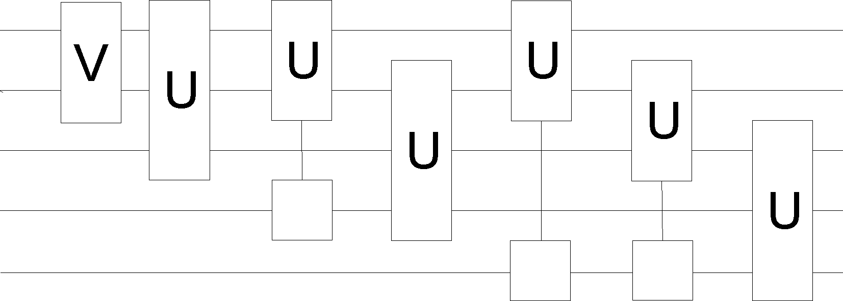
Figure 1: Sequence of gates of compression transformation in the five-qubits example. Operation $V$ represents the starting two-qubit transformation (10) and operations $U$ represent relevant $U(a,b)$ operations (12).

IV Final step

As a final step of the procedure, we need to perform a transformation

$$\left|C\right\rangle_{k}\longrightarrow\left|B\right\rangle_{k},$$ (20)

where $\left|B\right\rangle_{k}$ is a set of $N+1$ states occupying nontrivially only the subspace of $\left\lceil\log(N+1)\right\rceil$ qubits. As a natural suggestion we define the states as binary notation of the number $k$. E.g. for every $k$, the state $\left|B\right\rangle_{k}$ will have excited those qubits, which stand on positions, on which in the binary notation of the number $k$ is a $1$. On all other positions the qubits will be in the ground state. The state $\left|B\right\rangle_{k}$ will have the form

$$\left|B\right\rangle_{k}=\left|0\right\rangle^{\otimes(N-\left\lceil\log(N+1)\right\rceil)}\left|b\right\rangle_{k},$$ (21)

where $\left|b\right\rangle_{k}$ is a state of $\left\lceil\log(N+1)\right\rceil$ qubits. After the whole procedure, we can simply discard most of the qubits and keep only a logarithmic number of them, still keeping the whole information.

Now the main task is to perform the transformation efficiently, e.g. with at most polynomial number of elementary gates. This seems not to be a crucial problem, as we will work strictly in the computational basis, i.e. perform only transformations from one basis state to other basis state. Similarly to the previous transformation, we will perform it consecutively from the first to the last qubit. First of all, let us remark that for $k<3$ the transformation is trivial and no action is needed. The first non-trivial number is $k=3$ where we need to transform $\left|0\right\rangle^{\otimes(N-3)}\left|100\right\rangle\longrightarrow\left|0\right\rangle^{\otimes(N-3)}\left|011\right\rangle.$ This can be done easily by performing two C-NOT gates with the third qubit as control and the first and second qubit as targets. After that, we can perform a Toffoli gate with the first and second qubits as controls and third qubit as target. Obviously, these gates will act nontrivially only on the desired state, as all other states $\left|C\right\rangle_{k}$ with $k\neq 3$ have $\left|0\right\rangle$ on the third position. All states with $k\neq 3$ do not have $\left|1\right\rangle$ both on first and second position.

For $k>3$ we will perform similar operations. For every $k$ we will perform C-NOT gates with the $k$th qubit as control and those qubits as targets, which represent the number $k$ in binary notation. At the end we will perform a single Toffoli gate with all these (target) qubits as control, all other qubits on positions smaller than $k$ as reversed controls (initiating the operation if in the state $\left|0\right\rangle$) and the $k$th qubit as target. If we perform these operations subsequently from smaller to bigger $k$ (from $3$ to $N$), they will always act nontrivially only on the relevant state $\left|C\right\rangle_{k}$.

For every $k$, we will need to perform at most $\log(k)$ C-NOT gates and one Toffoli gate with $\log(k)$ controls. Such a Toffoli gate can always be performed with quadratic number of C-NOT gates Kniznica (6) with respect to the number of control qubits. So, for every $k$, we need roughly $\log^{2}(k)$ C-NOT gates. Thus for the whole transformation we will need no more gates that in the order of

$$\sum_{k=3}^{N}\log^{2}(k)<\sum_{k=3}^{N}\log^{2}(N)<N\log^{2}(N)$$

C-NOT gates.

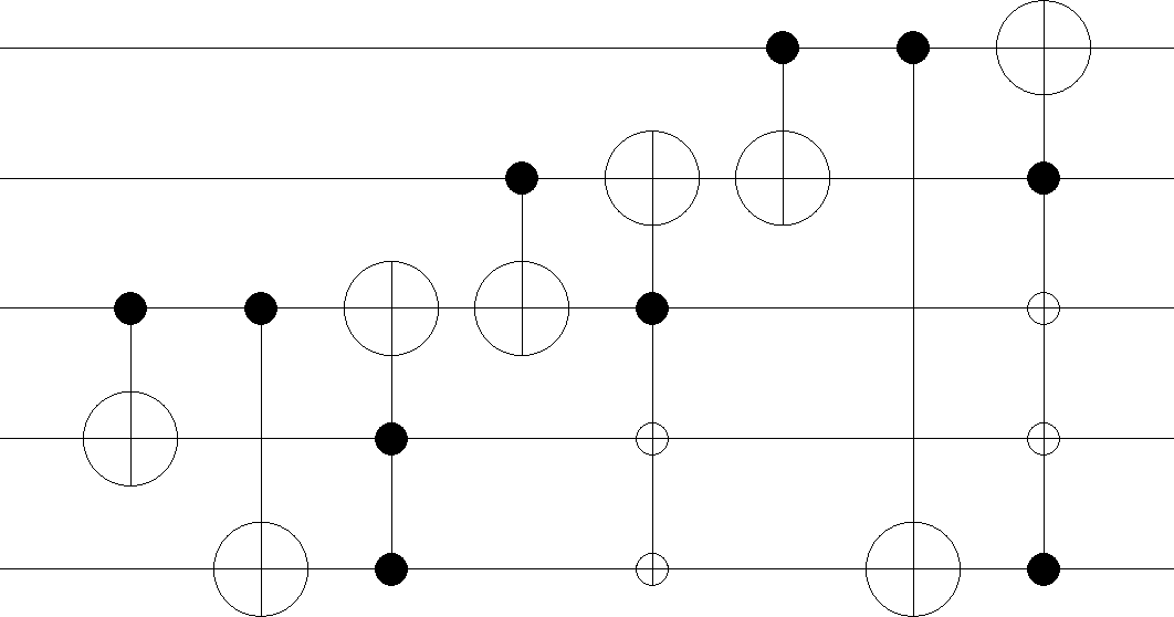
Figure 2: Sequence of gates for the final step operation in the five-qubit example.

V Noise analysis

To show the capabilities of compressed state to resist to specific noise, we have performed analysis on a specific noise model. Within this model, every qubit is unitarily rotated by a specific angle $\phi$ around a defined axis on the Bloch sphere. Such noise can be imagined to be active, e.g. a magnetic field causing precession of the stored (or sent) qubits. In the same way a passive ”noise” can be imagined, causing rotation or misalignment of the reference frames.

We consider two scenarios. In first scenario, all $N$ qubits are stored without compression and noise is acting an all the qubits. In second scenario we first compress the $N$ qubits and store only the non/trivial part of the state. The noise is acting now only on the stored qubits. At the end we add qubits in the state $\left|0\right\rangle$ and decompress the state.

The decompression procedure is fully defined only for $N=2^{k}-1$ for every $k>0$. In other cases, the Hilbert space of the compressed system has dimensions not used for storing information, the unperturbed compressed state has zero amplitudes within this dimensions. However, the noise can rotate the compressed state such that also these dimension are used and in such a case one would have to define the decompressing operation further to cover the whole Hilbert space of compressed state.

V.1 Global state fidelity

Fidelity of the global state (1) between the original, unperturbed state with the state after action of noise an all qubits is compared to the fidelity of state after compression, action of noise and decompression. We average over all possible input states of qubits and over all axis of rotation of the noise. The results for $\phi=0.1rad$ and different number of qubits are shown in the Figure (3). In this case the dimensions of the Hilbert space of compressed state not used for storing information will never contribute the the fidelity and therefore we do not have to further define the decompression operation.

On the figure a clear structure is seen for the compressed state with maximums of fidelities for specific number of qubits (3,7,15). These are numbers for which the whole Hilbert space of compressed state is used to store information. By increasing the number of qubits, a sudden drop of fidelity appears due to increase of the number of qubits of the compressed state, which are subject to the action of noise. In any situation the fidelity of the state after compression-decompression procedure is higher than in the naive scenario of storing all qubits.

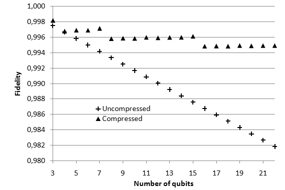
Figure 3: Fidelity of global state after the action of noise with and without compression and decompression. The fidelity of the compressed state is clearly higher than the fidelity of the uncompressed one.

V.2 Single qubit fidelity

Here the fidelity of the single qubit state is examined under the scenarios described above (with and without compression). In this case the unused dimensions in the Hilbert space of compressed state play may contribute to the result, therefore we examined a specific case of $N=7$, where this is not the case. The symmetry of the operation as well as of the errors guarantee the symmetry of the resulting state. In general the state after decompression will be entangled, resulting in mixed one qubit states, but still all of them identical.

The results o the calculations are shown in the Figure 4) for different values of $\phi$. Results are averaged through all input states. For uncompressed state the resulting fidelity is not dependent on the axis of rotation of the error. However, this is not the case for the compressed state, therefor results for three specific axes of rotation, as well as the result after averaging over all possible axes is shown.

We can conclude that in general the modelled type of noise is more harmful to stored qubits. However, as only a small amount of qubits is stored in the compressing scenario in comparison the naive scenario, one can expect the ability to guarantee smaller average errors. Even with the same error rate, we can obtain better fidelity in the compressing scenario. If we have a prediction about one more-stable axis, we can choose this to be the $z$ axis of the compression-decompression operation (defining the computational base and C-NOT operation). For errors causing rotation around this axis the compressed state is more stable then the uncompressed one.

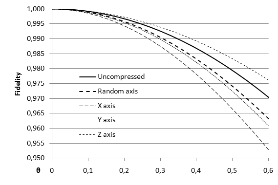
Figure 4: Fidelity of one qubit state after the action of noise with and without compression and decompression. For compression scenario, results for noise acting around $x$, $y$ and $z$ axes, as well as for noise averaged through all axes are shown.

VI Conclusions

In this paper we have suggested a quantum compression scheme for transformation of an $N$-fold product state of a single qubit state into a state, which is non-trivial only on $\left\lceil\log(N+1)\right\rceil$ qubits. The same procedure also describes the inverse operation (decompression). Both of these are effective in a sense that only $O(N^{2})$ C-NOT gates are needed to perform the operations.

Possible use of the scheme is a quantum memory. Having more copies of a single-qubit state, it might be very reasonable to compress them into a state of only a few qubits, which will be more easily protected against decoherence. If the copies are needed again, we perform the decompression transformation.

In fact, if the stored state is exposed to errors causing a rotation of the basis, a loss of fidelity is observed. If we compare the scenario of storing uncompressed qubit states with the scenario of storing the compressed state, the error (expressed in the loss of fidelity) is significantly smaller in the latter case Errors (12). This is true even for big errors, where standard error-correcting procedures fail.

The scenario of storing quantum information is imaginable e.g. in a case when a single-qubit state is a result of a stage of quantum computation and is needed as an input for a following stage of the computation. If some stages of the computation can not be performed immediately after each other (they may use the same “hardware” which needs to be adjusted etc.), the $N$-fold symmetric state of a single-qubit state (obtained after $N$ runs of the computation) may be compressed and stored effectively, e.g. with exponentially smaller memory demands and lower error rate, in the meantime.

Another possible application is the sending of information about a direction using quantum states. In cases when two communicating parties share a reference frame, states resulting from the suggested compression are very effective in communicating the direction. If the sender has an option to send at most $n$ qubits, he prepares a $2^{(n-1)}$-fold symmetric state of a single-qubit state pointing in the desired direction. After compression, the resulting compressed state will span the Hilbert space of exactly $n$ qubits and can be sent to the receiver. He will now decompress it back into $2^{(n-1)}$-fold symmetric state of a single-qubit state and perform standard state tomography.

To compare the power of the suggested compression scheme with known procedures, fidelities of sending of a direction via a quantum channel using a small number of qubits are presented in the Table 2. For big number of qubits, the fidelity of our procedure grows as $F=1-\frac{1}{2^{n}+2}$, which is exponentially faster than $F\sim 1-\frac{\xi}{n^{2}}$ for the scheme presented in Bagan (3) or for the case of sending simple copies of the qubit state, where $F=$ $1-\frac{1}{n+2}$ Fidelity (13). Thus by utilizing a shared reference frame between communicating parties and paying the cost of it we can gain an exponential decrease of fidelity loss.

n	1	2	3	4	5	6
$\left|\psi\right\rangle^{\otimes n}$	$0.666$	$0.750$	$0.800$	$0.833$	$0.855$	$0.875$
EB	$0.666$	$0.789$	$0.845$	$0.911$	$0.931$	$0.943$
PB	$0.666$	$0.800$	$0.889$	$0.941$	$0.970$	$0.992$

Table 2: The comparison of fidelities of transfer of a direction using quantum states in cases of a naïve scenario – transfer of multiple copies of a single qubit, the Bagan et. al. scheme [3] (EB) and our compression scheme (PB).

Acknowledgments. This work was supported by the Slovak Research and Development agency project APVV-0673-07. We thank Michal Sedlák for helpful discussions and Marcela Hrdá for numerical analysis. MP would like to thank Action Austria-Slovakia for support.

References

- (1) N. Gisin and S. Popescu, PRL 83, 432 (1999)
- (2) S. Massar, PRA 62, 040101(R), (2000)
- (3) E. Bagan, M. Baig, A. Brey, R. Munoz-Tapia, R. Tarrach, PRL 85, 5230 (2000)
- (4) M. A. Nielsen, I. L. Chuang, Quantum Computation and Quantum Information, Cambridge university press (2000)
- (5) D. Bacon, I. L Chuang, A. W. Harrow, quant-ph/0601001 (2006) and references therein
- (6) A. Barenco et.al., PRA 52, 3457 (1995)
- (7) P. Kaye and M. Mosca, quant-ph/0101009 (2001)
- (8) P. Kaye and M. Mosca, quant-ph/0407102 (2004)
- (9) V. Shende, S. Bullock and I. Markov, IEEE Transactions on Computer-Aided Design 25 no. 6, 1000 (2006)
- (10) V. Bergholm, J. Vartiainen, M. Mottonen and M.Salomaa, Phys. Rev. A 71, 052330 (2005)
- (11) M. Sedlak and M. Plesch, CEJP, 6(1) 2008, 128-134 (2008)
- (12) M. Plesch and M. Hrda, in preparation
- (13) S. Massar and S Popescu, PRL 77, 1259 (1999)