Boltzmann equation and hydrodynamic fluctuations

Abstract

We apply the method of invariant manifolds to derive equations of generalized hydrodynamics from the linearized Boltzmann equation and determine exact transport coefficients, obeying Green-Kubo formulas. Numerical calculations are performed in the special case of Maxwell molecules. We investigate, through the comparison with experimental data and former approaches, the spectrum of density fluctuations and address the regime of finite Knudsen numbers and finite frequencies hydrodynamics.

I Introduction

The Boltzmann equation (BE) lies at the basis of classical and quantum kinetic theory of gases. It provides a detailed picture of the time evolution of a dilute gas towards a thermal equilibrium state, which constitutes the essence of the H-theorem. This celebrated result gave rise, historically, to the first clear insurgence of irreversibility into deterministic equations of motion. The nonlinear integro-differential nature of the BE prevented, so far, an exact solution. Perturbative methods and kinetic toy models have been devised such to get partial answers. The Chapman-Enskog expansion (CE) was, in particular, the first important success in this direction chapman , as it allowed to consistently derive hydrodynamics laws from their microscopic counterpart and to obtain rigorous expressions for transport coefficients. The CE method is based upon a perturbative expansion of the distribution function in terms of the Knudsen number $\varepsilon$, defined as the ratio between the mean free-path and a macroscopic hydrodynamic length. This is supposed to be a “smallness” parameter, in that the series converges only for $\varepsilon\rightarrow 0$. By increasing the order of the expansion one should not expect to capture larger extents of the “true” solution of the BE, since, as it was pointed out by Bobylev Bobylev82 , one has to face divergencies of the acoustic modes in the dispersion relation, which are inherently related to the procedure of truncation. In order to tackle this unphysical feature of post-Navier Stokes hydrodynamics, some regularization methods were borrowed from functional analysis in order to restore the H-Theorem Bobylev06 . Another route, which attempts a non–perturbative approach to solve the BE, is based upon the notion of Invariant Manifold karlinbook . Through this method, one assumes a priori a separation of the hydrodynamic time scale and the kinetic time scale and postulates the existence of a stable Invariant Manifold (IM) in the space of distribution functions, which is parameterized with the values of the hydrodynamic fields: particle number, velocity, and temperature. In this paper we address the study of the spectrum of hydrodynamic excitations in a Maxwell gas, employing the latter non–perturbative approach, which will allow to find exact transport coefficients at arbitrary length scales. The paper is organized as follows: in Sec. II we review the eigenvalue problem associated with the linearized Boltzmann equation and recall that hydrodynamic modes at finite wavevector can be obtained as eigenvalues of a perturbed linear operator. Next, in Sec. III, we motivate and derive the invariance equations (details collected in Appendix A) and consider the case of Maxwell molecules (Sec. III.1), whose associated eigenvalue problem for the unperturbed operator is analytically solvable (Appendix B). Postulating the existence of an IM, we solve the eigenvalue problem for arbitrary wavevectors and find generalized transport coefficients which recover the Green-Kubo formulas in Sec. III.2. Further, in Section IV, we determine the spectrum of density fluctuations and formulate a hypothesis about the features of finite wavelengths hydrodynamics. Conclusions are drawn in Sec. V.

II Eigenvalue problems for the Boltzmann equation and hydrodynamics

The dynamics of the fluctuations of hydrodynamic fields (particle number, momentum, temperature) as induced by the properties of the underlying microscopic or kinetic equation, is an important issue in statistical mechanics which dates back to the seminal work by Onsager Onsager . In this section we focus upon the BE and show in a general setting how it features equilibration through some generalized frequencies (inverse of characteristic collision times). The way how these generalized frequencies give rise and affect the decay rates of some collective fluctuations (hydrodynamic modes) of the macroscopic fields, is still an issue which lacks a rigorous foundation. The reason is that the hydrodynamic equations, as derived from the BE, are not closed and hence, some (semi-phenomenological) approximations for higher order moments need to be included. In particular, the celebrated Navier-Stokes-Fourier (NSF) approximation was the first historically relevant attempt in this direction. We start by reviewing some results formerly obtained by Resibois resibois . He shed some preliminary light upon the connection between the generalized frequencies and the hydrodynamic modes by solving, via perturbation theory, the eigenvalue problems associated independently to the BE and to the NSF equations of hydrodynamics.

II.1 The Boltzmann equation

The BE reads:

$$\partial_{t}f=-\textbf{v}\cdot\nabla f+Q[f,f],$$ (1)

where $Q$ denotes a non-linear integral collision operator. We introduce the thermal velocity $v_{T}=\sqrt{2k_{B}T_{0}/m}$, the dimensionless peculiar velocity $\textbf{c}=(\textbf{v}-\textbf{u}_{0})/v_{T}$ and the equilibrium values of macroscopic fields: equilibrium particle number $n_{0}$, equilibrium mean velocity $\textbf{u}_{0}=\textbf{0}$, and equilibrium temperature $T_{0}$. The global Maxwellian is defined as: $f^{\textrm{GM}}=(n_{0}/v_{T}^{3})f_{0}(c)$ where $f_{0}(c)=\pi^{-3/2}e^{-c^{2}}$ denotes a Gaussian in velocity space ($c\equiv|\textbf{c}|$). We consider only small disturbances from the global equilibrium. After passing over to Fourier space, we write the distribution function (cf. also Tab. 1) as:

$$f(\textbf{k},\textbf{c},t)=f^{\textrm{LM}}+\delta f,$$ (2)

where $f^{\textrm{LM}}$ denotes the local Maxwellian to be made precise in Sec. III, and $\delta f$ the deviation from local equilibrium. An alternative notation is introduced via $\delta f=f^{\textrm{GM}}\delta\varphi$. Considering a co-moving reference frame and linearizing the collision operator around global equilibrium, one obtains from (1)

$$\frac{1}{v_{T}}\partial_{t}f=-i\textbf{k}\cdot\textbf{c}f+\hat{L}\delta f,\qquad\hat{L}=\frac{1}{v_{T}}L,$$ (3)

where we made use of the fact that $Lf^{\textrm{LM}}=0$. The linearized Boltzmann collision operator, $L$, assumes the form

$$L\delta f = \int\int d\Omega d\textbf{c}_{1}\sigma(\Omega,g)gf^{\textrm{GM}}(c_{1})\times$$ (4)

$$[\delta\varphi(\textbf{k},\textbf{c})+\delta\varphi(\textbf{k},\textbf{c}_{1})-\delta\varphi(\textbf{k},\textbf{c}^{\prime})-\delta\varphi(\textbf{k},\textbf{c}_{1}^{\prime}].$$

Here, $\sigma(\Omega,g)$ is the scattering cross section, $g\equiv|v-v_{1}|$, and $v$, $v_{1}$ are the velocities of the particles entering the binary collision. In the remainder ot this section, we will focus our attention upon the operator $\mathrm{\Lambda}\equiv\hat{L}-i\textbf{k}\cdot\textbf{c}$, whose spectral properties determine the time evolution of the distribution function. This is readily seen by considering the Laplace time transform of Eq. 3 (to be further discussed in Sec. IV) and by inspection of the inverse transform, which reads as:

$$f(\textbf{k},\textbf{c},t)=\frac{1}{2\pi i}\oint\frac{e^{zt}}{(z-\mathrm{\Lambda})}dzf(\textbf{k},\textbf{c},0),\\$$ (5)

where the closed path encircles all the poles of the integrand function. Through the Spectral Theorem, we regard these poles as coinciding with the spectrum of the operator $\mathrm{\Lambda}$. The investigation of the spectral properties of such an operator is, in fact, a longstanding issue in kinetic theory Blatt . In order to study the eigenvalue problem associated with $\Lambda$, we introduce the Fourier time transform of the distribution function $f(\textbf{k},\textbf{c},\omega)=\int_{-\infty}^{\infty}e^{-\omega t}f(\textbf{k},\textbf{c},t)dt$, where $\omega$ defines a complex valued quantity. Then, (3) reduces to:

$$\Lambda f=\omega f,$$ (6)

which constitutes the starting point of our analysis.

In the present paper, functions $f_{\mu}=f^{\textrm{GM}}\varphi_{\mu}$ will be regarded as vectors in a Hilbert space, whose scalar product is defined by:

$$\langle f_{1}|f_{2}\rangle=\frac{1}{n_{0}}\int(f^{\textrm{GM}})^{-1}f_{1}(\textbf{c})f_{2}(\textbf{c})d^{3}v.$$ (7)

The spectrum of $\Lambda$ is analytic in $k=0$ and it can be shown to contain a $D+2$–fold degeneracy at the origin, corresponding to local conserved quantities. In order to solve the eigenvalue problem associated with (6), it is worth first to attempt the analysis of the long-wavelength limit $k\rightarrow 0$:

$$\hat{L}\Psi_{i}(\textbf{c})=\lambda_{i}\Psi_{i}(\textbf{c}).$$ (8)

The operator $\hat{L}$ is found to be symmetric and negative semidefinite with respect to the scalar product (7), hence eigenfunctions are orthogonal and form a complete set. In particular, a subset of them, which spans a $(D+2)$–dimensional subspace of the Hilbert space can be found corresponding to the degenerate zero eigenvalue. These are the collision invariants $f^{\textrm{GM}}{\bf X}^{0}$, with ${\bf X}^{0}$ denoting a set of lower order Sonine (or associated Laguerre) polynomials:

$${\bf X}^{0}=\left[1,2\textbf{c},\left(c^{2}-\frac{3}{2}\right)\right]$$ (9)

(see also Eq. 41a). A perturbative approach is followed in order to extract those eigenvalues, denoted hereafter by $\omega_{\textrm{hydro}}$, which reduce to zero in the long wavelength limit, from the full spectrum of $\Lambda$. The yet unknown eigenfunctions and eigenvalues are expanded in powers of the wavevector k:

$$|\Psi_{\alpha}\rangle = |\Psi_{\alpha}^{(0)}\rangle+k|\Psi_{\alpha}^{(1)}\rangle+k^{2}|\Psi_{\alpha}^{(2)}\rangle+\dots,$$

$$\omega_{\alpha} = \omega_{\alpha}^{(0)}+k\omega_{\alpha}^{(1)}+k^{2}\omega_{\alpha}^{(2)}+\dots,$$ (10)

where $|\Psi_{\alpha}^{(0)}\rangle$ denotes a linear combination of the eigenfunctions of the unperturbed system. The result of this standard procedure is a polynomial expression for the set $\{\omega_{\alpha}\}$ of hydrodynamic modes, up to second order:

$$\omega_{1} = ic_{0}k-k^{2}\langle\Psi_{1}^{(0)}|(c_{x}-c_{0})\frac{1}{\hat{L}}(c_{x}-c_{0})|\Psi_{1}^{(0)}\rangle,$$

$$\omega_{2} = -ic_{0}k-k^{2}\langle\Psi_{2}^{(0)}|(c_{x}+c_{0})\frac{1}{\hat{L}}(c_{x}+c_{0})|\Psi_{2}^{(0)}\rangle,$$

$$\omega_{3} = -k^{2}\langle\Psi_{3}^{(0)}|c_{x}\frac{1}{\hat{L}}c_{x}|\Psi_{3}^{(0)}\rangle,$$

$$\omega_{4} = -k^{2}\langle\Psi_{4}^{(0)}|c_{x}\frac{1}{\hat{L}}c_{x}|\Psi_{4}^{(0)}\rangle,$$

$$\omega_{5} = -k^{2}\langle\Psi_{5}^{(0)}|c_{x}\frac{1}{\hat{L}}c_{x}|\Psi_{5}^{(0)}\rangle,$$ (11)

where $c_{0}=(5k_{B}T_{0}/3m)^{\frac{1}{2}}$ is the speed of sound of an ideal gas.

$f$	=	$f^{\textrm{LM}}$			+	$\delta f$
		$\overbrace{\hskip 99.58464pt}$
	=	$f^{\textrm{GM}}$	+	$f^{\textrm{GM}}\varphi_{0}$	+	$f^{\textrm{GM}}\delta\varphi$
	=	$f^{\textrm{GM}}$	$+$	$f^{\textrm{GM}}{\bf X}^{0}\cdot\textbf{x}$	+	$f^{\textrm{GM}}\delta{\bf X}\cdot\textbf{x}$
				$\underbrace{\hskip 136.5733pt}$
	=	$f^{\textrm{GM}}$	$+$	$f^{\textrm{GM}}\triangle{\bf X}\cdot\textbf{x}$
	=	$f^{\textrm{GM}}$	$+$		$\triangle f$

Table 1: Notation used in this manuscript. Terms have been grouped and abbreviated as depicted in this table. $f^{\textrm{GM}}$ and $f^{\textrm{LM}}$ denote global and local maxwellian, respectively, and $\triangle f$ and $\delta f$ their “distance” from $f$. The third row informs about the closure discussed in this manuscript, while x is a set of lower order moments of $f$.

II.2 Linear Hydrodynamics

We denote by $[n_{k},\mathbf{u}_{k},T_{k}]$ the Fourier transforms of the hydrodynamics fields, for instance: $n_{k}=\int_{-\infty}^{\infty}dt\int_{-\infty}^{+\infty}d\mathbf{r}e^{-\omega t-i\mathbf{k}\cdot\mathbf{r}}\delta n(\mathbf{r},t)$, where $\delta n(\mathbf{r},t)$ is the fluctuation at time $t$ and point $\mathbf{r}$ of the local particle number. The equations of hydrodynamics considered in resibois , are the linearized Navier-Stokes-Fourier (NSF) equations, which represent balance equations for particle number density, momentum and kinetic energy endowed with specific constitutive equations for the stress tensor and heat flux:

$$\omega n_{k}(\omega) = -in_{0}\mathbf{k}\cdot\mathbf{u}_{k}(\omega),$$ (12a)

$$\omega\mathbf{u}_{k}(\omega) = -i\frac{\mathbf{k}}{n_{0}}\left(\frac{\partial P}{\partial n}\right)_{T}n_{k}(\omega)-i\frac{\mathbf{k}}{n_{0}}\left(\frac{\partial P}{\partial T}\right)_{n}T_{k}(\omega)$$ (12b)

$$-\frac{\eta}{n_{0}}k^{2}\mathbf{u}_{k}(\omega)-\frac{\mathbf{k}}{n_{0}}\left(\zeta+\frac{1}{3}\eta\right)\mathbf{k}\cdot\mathbf{u}_{k}(\omega),$$

$$\omega T_{k}(\omega) = -i\frac{1}{n_{0}}\frac{T_{0}}{C_{v}}\mathbf{k}\cdot\mathbf{u}_{k}(\omega)-\frac{\kappa}{C_{v}n_{0}}k^{2}T_{k}(\omega),$$ (12c)

where $\zeta$ and $\eta$ are respectively the bulk and shear viscosity, $C_{v}$ is the specific heat at constant volume and $\kappa$ is the thermal conductivity. Solving the Eqs. (12) amounts to determine the eigenvalues of a $5\times 5$ non Hermitian matrix, which represent the decay rates of the collective excitations. The intuition enlightened in the paper resibois was to put into correspondence the macroscopic eigenvalues with their microscopic counterpart, obtained from (8) by application of perturbation theory. This identification allowed to find an approximate expression for transport coefficients only in terms of the one-body distribution function which turned out to be equivalent to reduced expressions determined by many-body autocorrelation functions. These coefficients properly recover the Chapman-Enskog expressions from classical kinetic theory. Within the above construction it is found that the decay rates of hydrodynamic modes in the NSF approximation are quadratic in the wave vector Re$(\omega)\propto-k^{2}$ and unbounded. The use of a suitable projector, on the other hand, outlined in the next section, allows us to find proper asymptotics and paves the way to solve the eigenvalue equation (6) as well as to determine exact transport coefficients.

III The Invariant Manifold technique

The notion of invariant manifold is a generalization of normal solution in the Hilbert and Chapman-Enskog method. Given a dynamical system

$$\frac{df}{dt}=J(f),$$ (13)

where $J(f)$ is the vector field which induces the motion in the space of distribution functions U. Given bounded and smooth functions $\textbf{x}(\textbf{r},t)$ we define the locally finite-dimensional manifold $\Omega\subset\textit{U}$ as the set of functions $f(\textbf{x}(\textbf{r},t),\textbf{c})$. Hence, we will only consider sets of distribution functions whose dependence upon the space variable r is parameterized through some “moments” $\textbf{x}(\textbf{r},t)$. As it will be discussed in Sec. IV, once we identify such coarse-grained fields $\textbf{x}(\textbf{r},t)$ with the hydrodynamic fields, postulating their existence corresponds to invoking the hypothesis of local thermodynamic equilibrium. Hence, the extent of our predictions is inherently restricted to lenght scales wherein the concept of a field as ensemble average over a statistically significant number of particles is still meaningful. Let us denote by $T_{w}$ the tangent space to the manifold $\Omega$ at the point $w$ of the phase space, and let us introduce a projection operator $P$ which, when acting on $J(f)$, describes the motion of the vector field along the manifold. The dynamics is, hence, splitted into a fast motion on the affine subspace $w+\textrm{ker}[P]$ and a slow motion, which occurs along the tangent space $T_{w}$ karlinbook . The set of eigenvalues $\omega_{\textrm{hydro}}$ is determined as follows:

1. We seek for an invariant manifold $\Omega\subset\textit{U}$ such that the following Invariance Equation (IE) is fulfilled:

   $$(\textbf{1}-P)\Lambda\Delta f=0$$ (14)

   where $\triangle f\equiv f-f^{\textrm{GM}}$ (cf. also Tab. 1).

2. After determining the nonequilibrium distribution function from Eq. (14), we derive equations of linear hydrodynamics via integration of the kinetic equation (3). By construction, the decay rates of the macroscopic excitations then coincide with $\omega_{\textrm{hydro}}$.

Let $\textbf{x}=[\tilde{n},\tilde{\textbf{u}},\tilde{T}]$ denote the set of dimensionless hydrodynamic fluctuations: $\tilde{n}\equiv(n-n_{0})/n_{0}=$ (particle number perturbation), $\tilde{\textbf{u}}\equiv\textbf{u}/v_{T}=$ (velocity perturbation) and $\tilde{T}\equiv(T-T_{0})/T_{0}$ (temperature perturbation). Further, we split the mean velocity $\tilde{\textbf{u}}$ uniquely as $\tilde{\textbf{u}}=u^{\mbox{\tiny$\|$}}{\bf e}_{\mbox{\tiny$\|$}}+u^{\mbox{\tiny$\bot$}}{\bf e}_{\mbox{\tiny$\bot$}}$, where the unit vector ${\bf e}_{\mbox{\tiny$\|$}}$ is parallel to k, and ${\bf e}_{\mbox{\tiny$\bot$}}$ orthonormal to ${\bf e}_{\mbox{\tiny$\|$}}$, i.e., ${\bf e}_{\mbox{\tiny$\bot$}}$ lies in the plane perpendicular to k. Due to isotropy, $u^{\mbox{\tiny$\bot$}}$ alone fully represents the twice degenerated (shear) dynamics. By linearizing around the global equilibrium, we write the local Maxwellian contribution to $f$ in (2) as $f^{\textrm{LM}}=f^{\textrm{GM}}(1+\varphi_{0})$ where $\varphi_{0}$ takes a simple form, $\varphi_{0}={\bf X}^{0}\cdot\textbf{x}$ (linear quasi equilibrium manifold), where ${\bf X}^{0}(\textbf{c})$ was defined in Eq. (9). It is conveniently considered as four–dimensional vector using the four–dimensional version $\textbf{x}=[\tilde{n},u^{\mbox{\tiny$\|$}},\tilde{T},u^{\mbox{\tiny$\bot$}}]$, and is then given by (41a). It proves convenient to introduce a vector of velocity polynomials, $\mbox{\boldmath{$\xi$}}(\textbf{c})$, which is similar to ${\bf X}^{0}$ and defined by (41b), such that $\langle f^{\textrm{GM}}\xi_{\mu}|f^{\textrm{GM}}X^{0}_{\nu}\rangle=\delta_{\mu\nu}$. Hence, the fields x are obtained as $\langle\mbox{\boldmath{$\xi$}}(\textbf{c})\rangle_{f^{LM}}=\textbf{x}$, where averages are defined as:

$$\left\langle\mbox{\boldmath{$\xi$}}(\textbf{c})\right\rangle_{f}=\frac{1}{n_{0}}\int\mbox{\boldmath{$\xi$}}(\textbf{c})f(\textbf{c})d^{3}\textbf{v}=\left\langle f^{\textrm{GM}}\mbox{\boldmath{$\xi$}}(\textbf{c})|f\right\rangle.$$ (15)

We introduce yet unknown fields $\delta{\bf X}({\bf c},\textbf{k})$ which characterize the part $\delta f$ of the distribution function. As long as deviations from the local Maxwellian stay small, we seek for a nonequilibrium manifold which is also linear in the hydrodynamic fields x themselves. Therefore, we set:

$$\delta\varphi=\delta{\bf X}\cdot\textbf{x}.$$ (16)

The “eigen”-closure (16), which formally and very generally addresses the fact that we wish to not include other than hydrodynamic variables, implies a closure between moments of the distribution function, to be worked out in detail below. By using the above form (16) for $\delta f=f^{\textrm{GM}}\delta\varphi$, with $\hat{L}\delta f=f^{\textrm{GM}}L[\delta{\bf X}]\cdot\textbf{x}$, and the canonical abbreviations $\triangle{\bf X}\equiv{\bf X}^{0}(\textbf{c})+\delta{\bf X}(\textbf{c},\textbf{k})$, Eq. (6) reads:

$$\omega f^{\textrm{GM}}\triangle{\bf X}\cdot\textbf{x}=\Lambda\Delta f=-i\textbf{k}\cdot\textbf{c}f^{\textrm{GM}}\triangle{\bf X}\cdot\textbf{x}+f^{\textrm{GM}}\hat{L}\delta{\bf X}\cdot\textbf{x}.$$ (17)

The microscopic projected dynamics is obtained from (14) by introducing the thermodynamic projection operator, defined in karlinbook , which, when acting upon $J(f)=\Lambda\Delta f$, gives:

$$P\Lambda\Delta f=D_{\textbf{x}}\Delta f\cdot\int\mbox{\boldmath{$\xi$}}(\textbf{c})\Lambda\Delta fd^{3}v,$$ (18)

where $D_{\textbf{x}}\Delta f\equiv\partial\Delta f/\partial\textbf{x}$ and the quantity inside the integral in (18) represents the time evolution equations for the moments x. These are readily obtained by integration of the weighted (6) as

$$\omega\langle\mbox{\boldmath{$\xi$}}(\textbf{c})\rangle_{f}=-i\textbf{k}\cdot\langle\mbox{\boldmath{$\xi$}}(\textbf{c})\textbf{c}\rangle_{f}+\langle\mbox{\boldmath{$\xi$}}(\textbf{c})\rangle_{\hat{L}\delta f}.$$ (19)

As shown in Tab. 1 , $D_{\textbf{x}}\Delta f=f^{\textrm{GM}}\triangle{\bf X}$ holds, whereas (19) is linear in x and can be written as $\omega\textbf{x}={\bf M}\cdot\textbf{x}$. Hence, Eq. (18) attains the form:

$$P\Lambda\Delta f=f^{\textrm{GM}}\triangle{\bf X}\cdot{\bf M}\cdot\textbf{x}.$$ (20)

In the derivation of (20), one needs to take into account that $\langle\mbox{\boldmath{$\xi$}}(\textbf{c})\rangle_{\delta f}={\bf 0}$ (as the fields x are defined through the local Maxwellian part of the distribution function only) and that $\langle\mbox{\boldmath{$\xi$}}(\textbf{c})\rangle_{\hat{L}\delta f}={\bf 0}$. The dependence of the matrix elements of $\bf M$ upon moments of $\delta f$ is explicitly given in Tab. 2. Combining (17) and (20), and requiring that the result holds for any x (invariance condition), we obtain a closed, singular integral equation (invariance equation) for complex-valued $\delta{\bf X}$,

$$\Delta{\bf X}\cdot{\bf M}=-i\textbf{k}\cdot\textbf{c}\,\triangle{\bf X}+\hat{L}\delta{\bf X}.$$ (21)

Notice that $\delta{\bf X}=\Delta{\bf X}-{\bf X}^{0}$ vanishes for $k=0$, which implies that the invariant manifold $\Omega_{k\rightarrow 0}$ in that limit is given by the set of local Maxwellians $f^{\textrm{LM}}$. The implicit equation (21) for $\delta{\bf X}$ (or $\Delta{\bf X}$, as ${\bf X}^{0}$ is known) is identical with the eigen-closure (16), and is our main and practically useful result. The Bhatnagar-Gross-Krook (BGK) collision model treated in matteo3 is recovered for $\hat{L}(\delta{\bf X})=-\delta{\bf X}$.

III.1 Solving the Invariance Equation

The invariance equation (21) as well as some symmetry relations for the components $\delta X_{\mu}$ of the nonequilibrium distribution functions (worked out in Appendix B for the interested reader) are exact. Solutions to this equation can be obtained in simple cases. Considering the BGK kinetic equation, for instance, the IE could recently be solved numerically and the spectrum of hydrodynamic modes at arbitrary wavelength has been successfully determined matteo3 . In the present case, our strategy to solve (21) is to confine ourselves with a special kind of interaction potential (Maxwell molecules) and is based upon the results obtained by Chang-Uhlenbeck uhlenbeck . They provided an analytical solution to the eigenvalue problem for the BE with the Maxwell molecules collision operator (i.e.: gas molecules interacting via a potential $V\propto r^{-4}$, see also JSP8 ). Their analysis showed that due to the isotropy of the operator $\hat{L}$ (i.e. it commutes with rotation operators in velocity space), it admits the following set of eigenfunctions $\Psi_{r,l}({\bf c})$,

$$\Psi_{r,l}=\sqrt{\frac{r!(l+\frac{1}{2})\sqrt{\pi}}{(l+r+\frac{1}{2})!}}\,c^{l}P_{l}(z)S_{l+\frac{1}{2}}^{(r)}(c^{2}),$$ (22)

where $P_{l}$ and $S_{l+\frac{1}{2}}$ denote, respectively, Legendre and Sonine polynomials, $c=|{\bf c}|$ and $z={\bf c}\cdot{\bf e}_{\mbox{\tiny$\|$}}/c$ (see also Appendix A). These eigenfuctions are orthonormal with respect to the scalar product (7), with corresponding eigenvalues:

$$\lambda_{r,l}=2\pi\int\sin(\vartheta)F(\vartheta)T_{r,l}(\vartheta)\,d\vartheta,$$ (23)

where the explicit expressions for the $F(\vartheta)$ and $T_{rl}(\vartheta)$ are needed to numerically solve (21) and hence delegated to Appendix A. Whereas the construction outlined in Sec. II deduces the eigenvalues of the perturbed system (8), which vanish in the $k\rightarrow 0$ limit, just from the knowledge of ker$[\hat{L}]$ (i.e., the “ground states” of the unperturbed system), here we attempt a different route. We introduce, first, a decomposition of the microscopic particle velocity, where its components can be expressed through the absolute value of velocity, $c$, and the cosine of the angle between velocity and wave vector, denoted as $z$, see (40). Next, we expand our functions $[{\bf X}^{(0)},\delta{\bf X}]$ in terms of the orthonormal basis $\Psi_{r,l}=\Psi_{r,l}(c,z)$:

$$X_{\mu}^{(0)}(c,z) = \sum_{r,l}^{N}a_{\mu}^{(0)(r,l)}\Psi_{r,l}(c,z),$$ (24a)

$$\delta X_{\mu}(k,c,z) = \sum_{r,l}^{N}a_{\mu}^{(r,l)}(k)\Psi_{r,l}(c,z).$$ (24b)

The equilibrium coefficients $a_{\mu}^{(0)}$ are known, and can be determined, by taking advantage of the orthogonality of the eigenfunctions, as:

$${\bf a}^{(0)(r,l)}=\pi^{-\frac{3}{2}}\int e^{-c^{2}}\Psi_{r,l}(c,z){\bf X}^{(0)}(c,z)\,d^{3}{\bf c}.$$ (25)

Inserting (24) into the IE (21), we obtain the following nonlinear set of algebraic equations for the unknown coefficients $a_{\mu}^{(r,l)}(k)$:

$$\left(a_{\nu}^{(r^{\prime},l^{\prime})}+a_{\nu}^{(0)(r^{\prime},l^{\prime})}\right)M_{\nu\mu}=$$ (26)

$$-i{\bf k}\cdot\sum_{r,l}^{N}\left(a_{\mu}^{(0)(r,l)}+a_{\mu}^{(r,l)}\right)\mbox{\boldmath{$\Omega$}}_{(r,l,r^{\prime},l^{\prime})}+\sum_{r,l}^{N}a_{\mu}^{(r,l)}\mathcal{L}_{(r,l,r^{\prime},l^{\prime})},$$

with:

$$\mathcal{L}_{(r,l,r^{\prime},l^{\prime})} = \langle f^{\textrm{GM}}\Psi_{r^{\prime},l^{\prime}}|\hat{L}|f^{\textrm{GM}}\Psi_{r,l}\rangle,$$ (27a)

$$\mbox{\boldmath{$\Omega$}}_{(r,l,r^{\prime},l^{\prime})} = \langle f^{\textrm{GM}}\Psi_{r,l}|\textbf{c}|f^{\textrm{GM}}\Psi_{r^{\prime},l^{\prime}}\rangle.$$ (27b)

For any order of expansion, the solutions of (26) characterize an invariant manifold in the phase space. The matrix elements $\mathcal{L}_{(r,l,r^{\prime},l^{\prime})}$ can be easily evaluated in few kinetic models, as for the BGK collision operator, hard spheres and Maxwell molecules. In particular, the latter case is recovered by setting:

$$\mathcal{L}^{\textrm{Maxw}}_{(r,l,r^{\prime},l^{\prime})}=\lambda_{r,l}\delta_{r,r^{\prime}}\delta_{l,l^{\prime}}.$$ (28)

Furthermore, the simplest case is BGK where all nonvanishing eigenvalues attain the constant value: $\lambda_{\textrm{BGK}}=-1$.

The calculation of the coefficients ${\bf a}^{(r,l)}$ is central in our derivation. Through these coefficients, the invariant manifold $\Omega\subset U$ is fully characterized: that is, the distribution function is determined and the corresponding matrix M of linear hydrodynamics is made accessible. Generalized transport coefficients such as viscosity and diffusion coefficients, defined in the Table 2, can be expressed in terms of these coefficients and they enter the definition of the stress tensor and heat flux (explicit expressions provided in Appendix A). In the regime of large Knudsen numbers the coefficients ${\bf a}^{(r,l)}$ may be further used to, e.g., directly calculate phoretic accelerations onto moving and rotating convex particles phoretic .

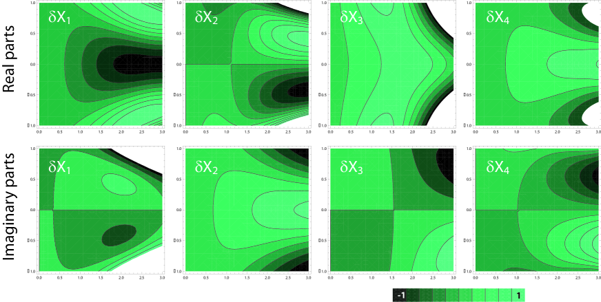
Figure 1: (Color online) All contributions $\delta X_{1-4}({\bf c},{\bf k})$ vs. $c$ (horizontal, $c=|{\bf c}|$) and $z\in[-1,1]$ (vertical axis, $z$ is the cosine of the angle between ${\bf k}$ and peculiar velocity ${\bf c}$) to the nonequilibrium distribution function $\delta f=f^{\textrm{GM}}\delta X_{\mu}x_{\mu}$ (16) at $k=1$, obtained with the fourth order expansion, $N=4$. Shown here are both their real (top) and imaginary parts (bottom row).

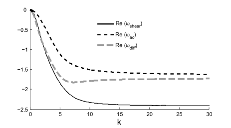
Figure 2: Hydrodynamic modes $\omega$ of the Boltzmann kinetic equation with Maxwell molecules collision operator as a function of wave number $k$. Shown are two complex conjugated acoustic modes $\omega_{\textrm{ac}}$, twice degenerated shear mode $\omega_{\textrm{sh}}$ and a thermal diffusion mode $\omega_{\textrm{diff}}$.

III.2 Hydrodynamic modes and transport coefficients

With ${\bf M}$ at hand, the hydrodynamic modes can finally be obtained from (20). The damping rates of the fluctuations (given by the real part of the hydrodynamic modes) are obtained by truncating the series (24) at the 4th order, and represented in Fig. 2. The first important finding is that, for any finite order of expansion, the modes extend smoothly over all the wavevector domain and, for large $k$, they attain an asymptotic value. This reflects the fact that, below a certain length-scale (more specifically, for lengths less than the mean free path), we reach the free-streaming limit, i.e., the regime in which the collisions cease to occur and particles move along straight lines. Hence, when reducing further the length scale, we may not expect an increase of the damping rate without the “thermalizing” effect of collisions. These physical arguments were already supported by the study of the BGK kinetic equation matteo3 , wherein the hydrodynamic modes, in the limit of small wavelengths, reach all the same value equivalent to the constant eigenvalue of the BGK collision operator. A further indication of the role played by the spectrum of $\hat{L}$ for large $k$ is provided by the observation that, when taking into account all the set of the eigenvalues of $\hat{L}$ which are unbounded below, also the hydrodynamic modes grow unboundedly.

Generalized transport coefficients are obtained by the nontrivial eigenvalues of $-k^{2}\textrm{Re}(\textbf{M})$: $\lambda_{2}=-A$ (elongation viscosity), $\lambda_{3}=-\frac{2}{3}Y$ (thermal diffusivity) and $\lambda_{4}=-D$ (shear viscosity). After some algebra it is possible to recast the expression for the higher order moments in terms of time correlation functions, in order to show the connection with the familiar Green-Kubo expressions. To this aim, we first write the nonequilibrium distribution function at time $\tau$ as:

$$\delta f(\textbf{k},\textbf{c},\tau) = e^{\Lambda\tau}\delta f(\textbf{k},\textbf{c},0).$$ (29)

$\sigma^{\mbox{\tiny$\|$}}_{1}$	$\sigma^{\mbox{\tiny$\|$}}_{2}$	$\sigma^{\mbox{\tiny$\|$}}_{3}$	$\sigma_{4}$
$\langle\lambda^{\mbox{\tiny$\|$}}\delta X_{1}\rangle$	$\langle\lambda^{\mbox{\tiny$\|$}}\delta X_{2}\rangle$	$\langle\lambda^{\mbox{\tiny$\|$}}\delta X_{3}\rangle$	$\langle c_{\mbox{\tiny$\|$}}c_{\phi}\delta Y_{4}\rangle$
$-k^{2}B$	$ikA$	$-k^{2}C$	$ikD$
real, $\oplus$	imag,$\oplus$	real,$\oplus$	imag,$\ominus$
$q^{\mbox{\tiny$\|$}}_{1}$	$q^{\mbox{\tiny$\|$}}_{2}$	$q^{\mbox{\tiny$\|$}}_{3}$	$q_{4}$
$\langle\gamma^{\mbox{\tiny$\|$}}\delta X_{1}\rangle$	$\langle\gamma^{\mbox{\tiny$\|$}}\delta X_{2}\rangle$	$\langle\gamma^{\mbox{\tiny$\|$}}\delta X_{3}\rangle$	$\langle(c^{2}-\frac{5}{2})c_{\phi}\delta Y_{4}\rangle$
$ikX$	$-k^{2}Z$	$ikY$	$-k^{2}U$
imag,$\ominus$	real,$\ominus$	imag,$\ominus$	real,$\oplus$

Table 2: Symmetry adapted components of (nonequilibrium) stress tensor $\sigma$ and heat flux ${\bf q}$, both introduced in (44). Row 2: Microscopic expression of these components (averaging with the global Maxwellian). Short-hand notation used: $\lambda^{\mbox{\tiny$\|$}}=c_{\mbox{\tiny$\|$}}^{2}-\frac{c^{2}}{3}$ and $\gamma^{\mbox{\tiny$\|$}}=(c^{2}-\frac{5}{2})c_{\mbox{\tiny$\|$}}$. Row 3: Expression of the components in terms of (as we show, real-valued) functions $A$–$Z$ (see text). Row 4: Parity with respect to $z$ – symmetric ($\oplus$) or antisymmetric ($\ominus$) – of the part of the corresponding $\delta X$ entering the averaging in row 2, and whether this part is imaginary or real-valued (see Fig. 1). Row 3 is an immediate consequence of row 4.

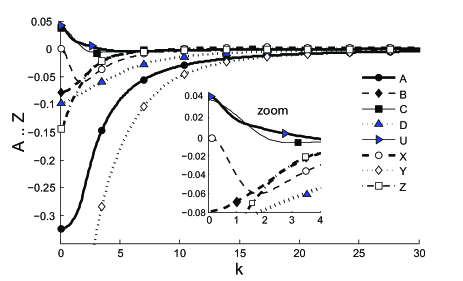
Figure 3: (Color online) Moments $A$-–$Z$ of the distribution function (see Tab. 2 and Eq. 45) vs. wave number $k$ obtained with the solution of (21). Non-triangles (black symbols): Moments entering only the longitudinal component of hydrodynamic equations. Triangles (blue symbols): Moments entering the transverse component of hydrodynamic equations.

Then, due to (24), by integrating both sides of (21), we find:

$$M_{\mu\nu} = \sum_{r,l}^{N}(a_{\nu}^{(0)(r,l)}\!+\!a_{\nu}^{(r)(r,l)})\langle f^{\textrm{GM}}\xi_{\mu}|\Lambda e^{\Lambda\tau}|f^{\textrm{GM}}\Psi_{r,l}\rangle$$ (30)

$$+\sum_{r,l}^{N}a_{\nu}^{(c)(r,l)}\langle f^{\textrm{GM}}\xi_{\mu}|\Lambda e^{\Lambda\tau}|f^{\textrm{GM}}\Psi_{r,l}\rangle,$$

where $a_{\nu}^{(r)(r,l)}$ and $a_{\nu}^{(c)(r,l)}$ are, respectively, real and imaginary–valued coefficients and $\langle f^{\textrm{GM}}\xi_{\mu}|\Lambda e^{\Lambda\tau}|f^{\textrm{GM}}\Psi_{r,l}\rangle=-ik\langle f^{\textrm{GM}}\xi_{\mu}|c_{\mbox{\tiny$\|$}}e^{\Lambda\tau}|f^{\textrm{GM}}\Psi_{r,l}\rangle$ because lower order moments of the collision operator identically vanish. Next, using the operator identity:

$$\Lambda e^{\Lambda\tau}=-\Lambda\left(\int_{\tau}^{\infty}e^{\Lambda t}dt\right)\Lambda,$$ (31)

we find for the real part of the M matrix in (30), for an arbitrary time $\tau=0$:

$${\rm Re}(M_{\mu\nu}) = -\sum_{r,l}^{N}a_{\nu}^{(c)(r,l)}\!\!\int_{0}^{\infty}\!\!dt\langle\dot{\xi}_{\mu}(0)\dot{\Psi}_{r,l}(t)\rangle_{f^{\textrm{GM}}},$$ (32)

where $\dot{\Psi}_{r,l}=\Lambda\Psi_{r,l}$. Equation (32) extends to arbitrary wave vector the Green-Kubo relations for transport coefficients. These relations hold in the hydrodynamic regime, when the system, as a result of many collisions, has reached local equilibrium. The opposite regime ($k\gg 1$) is represented by a simple gas of noninteracting point particles. Importantly, as it is evident from Fig. 3, and as already noticed in alder ; forster , the transport coefficients vanish in the limit of small wavelengths. This is due to the fact that the coefficients $a_{\nu}^{(r)(r,l)}$ and $a_{\nu}^{(c)(r,l)}$, solving (26), vanish in that limit. This vanishing character of transport coefficients (and, hence, of the heat flux and the stress tensor as is evident from Tab. 2) for large $k$, corresponds to Eulerian (inviscid) hydrodynamics. We are led, then, to similar conclusions to those traced when we discussed, in Sec. III, the $k\rightarrow 0$ limit of the invariance equation (14): in the free streaming regime, the local equilibrium manifold (local Maxwellian) becomes an invariant manifold. Let us recall that the Maxwellian distribution constitutes the zero point of the collision integral, in the sense that, in local equilibrium, the net flux of molecules entering and leaving an infinitesimal volume in space, due to the scattering processes, is zero. What we observe here is that, at a sufficiently short length-scale, the distribution function reduces to a Maxwellian, since the contribution from the scattering event, again, vanishes: but now this is because collisions ceased to occur.

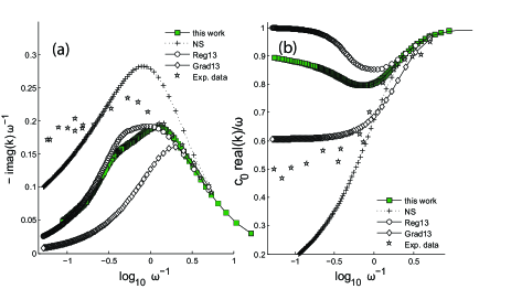
Figure 4: (Color online) (a) Damping spectrum, i.e., the negative imaginary part of $k$ divided by frequency $\omega$ vs. the negative logarithm of $\omega$. Results obtained in this work (by solving Eq. 21, and subsequently Eq. 20 for $w(k)$ with complex-valued $k$ and real-valued $\omega$) are compared with previous approaches including Navier Stokes (NS), regularized 13 moment (Reg13) Struchtrup07 , Grad 13 moment (Grad13), and experimental data presented in exprefmatteo . (b) Phase spectrum, i.e, real part of $k$ times velocity of sound $c_{0}$ and divided by $\omega$ vs. the negative logarithm of $\omega$. Again, we compare with reference results.

IV Finite wavelengths hydrodynamics

We raised the issue of the validity of the notion of invariant manifold for small wavelengths. We were able to show that hydrodynamic modes and the generalized transport coefficients extend smoothly over all the $k$–domain (there is no occurrence of any critical point as in the case of a Grad kinetic system, studied in CKK12 ); hence our approach, here and in matteo3 , tends to predict that the notion of invariant manifold holds also for short length scales. This would be in agreement with the celebrated papers by Alder et al. alder ; alder2 who considered a hard spheres gas and showed that hydrodynamic laws remain valid down to times comparable with the time between collisions, $t_{\textrm{coll}}$, and that the $k$-dependent zero frequency transport coefficients decay until they vanish at short length scales. It would be significant, therefore, to investigate the features of our model at finite frequencies and wavelegths and verify whether the procedure of truncation we introduced in (24) introduces a length scale below which our coarse-grained description breaks down. In Fig. 4 a comparison is shown about inverse phase velocity and damping for acoustic waves between our results, former approaches grad ; Struchtrup07 and experimental data performed by Meyer and Sessler exprefmatteo . As it is seen, our results are very close to the predictions of the regularized 13 (Reg13) moments method Struchtrup07 and closer to experimental data than Reg13 concerning the phase spectrum. Our theory is capable to predict that the phase speed remains finite also at high frequencies, a feature which is not possessed by any hydrodynamics derived from the CE expansion. A further clue about the features of our predictions in the regime of finite frequencies and wavevectors can be achieved by a closer inspection upon the spectrum of density fluctuations. To this aim, we introduce the Laplace transform of the hydrodynamic fields $\textbf{x}_{\textbf{k}}(z)=\int_{0}^{\infty}e^{-zt}\textbf{x}_{\textbf{k}}(t)dt$ and write the equation of linear hydrodynamics, analogously to (20), as:

$$\textbf{x}_{\textbf{k}}(z)=(z\textbf{I}-\textbf{M})^{-1}\textbf{x}_{\textbf{k}}(t=0).$$ (33)

By inverting the Laplace transform one obtains:

$$\textbf{x}_{\textbf{k}}(t)=\frac{1}{2\pi i}\oint\frac{e^{zt}}{(z\textbf{I}-\textbf{M})}dz\,\textbf{x}_{\textbf{k}}(t=0).$$ (34)

In order to proceed further and calculate the intermediate scattering functions $C_{\textbf{x},\textbf{x}}(\textbf{k},t)=\langle\textbf{x}_{\textbf{k}}(t)\textbf{x}_{-\textbf{k}}(0)\rangle$ it is needed, then, to define the averages which are employed in the calculation of correlation functions. These are, in fact, no longer ensemble averages, as in (15), but, due to (34), are averages over initial conditions, weighted by the probability density of thermodynamic fluctuation theory hansen ; sengers . Finally, the power spectrum of $C_{\textbf{x},\textbf{x}}$ is given by its Fourier transform:

$$S_{\textbf{x},\textbf{x}}(k,\omega)=\int_{-\infty}^{\infty}C_{\textbf{x},\textbf{x}}(\textbf{k},t)e^{-i\omega t}dt,$$ (35)

It is worth focusing upon the spectrum of density fluctuations, $S_{\tilde{n},\tilde{n}}$, as, being it related to the scattering cross-section, it is a quantity which is experimentally accessible. The calculation of $S_{\tilde{n},\tilde{n}}$ proceeds along the lines indicated above. It just suffices to notice how the solution for $\tilde{n}_{\textbf{k}}(z)$ involves terms proportional to the initial values of $\tilde{n}_{\textbf{k}},\tilde{\textbf{u}}_{\textbf{k}},\tilde{T}_{\textbf{k}}$, but, following standard recipes hansen , only the term proportional to $\tilde{n}_{\textbf{k}}(t=0)$ needs to be retained in the calculation. By considering just the lower order terms in $k$, one obtains:

$$\tilde{n}_{k}(t)=\left[\frac{2}{5}e^{-\chi k^{2}t}+\frac{3}{10}e^{-\Gamma k^{2}t}\cos(c_{0}kt)\right]\tilde{n}_{k}(0).$$ (36)

The first term in (36) represents a fluctuation which decays according to a purely diffusive process, with a lifetime proportional to $D_{T}$, whereas the second term represents a fluctuation propagating through the fluid at the (dimensionless) speed of sound $c_{0}=\sqrt{5/3}$ and decaying with a lifetime given by $\Gamma$. The coefficient $D_{T}$ generalizes the standard thermal conductivity, while $\Gamma$ generalizes the combined effect of both thermal conductivity and longitudinal kinetic viscosity. In the limit of small $k$, and following standard text books reichl , their expression is given by $D_{T}=\frac{2}{5}(X-Y)$ and $\Gamma=-(\frac{1}{2}A+\frac{1}{5}X+\frac{2}{15}Y)$. Unlike standard treatments of hydrodynamic fluctuations, the generalized transport coefficient $X$ enters the expression of the coefficients $D_{T}$ and $\Gamma$, even though its contribution, as it is evident from Fig. 3 is fairly small. The (approximate) intermediate correlation function is then obtained by averaging:

$$C_{\tilde{n},\tilde{n}}(\textbf{k},t) = \delta_{\textbf{k},0}+\langle\tilde{n}_{\textbf{k}}(0)\tilde{n}_{-\textbf{k}}(0)\rangle\times$$ (37)

$$\left[\frac{2}{5}e^{-D_{T}k^{2}|t|}+\frac{3}{10}e^{-\Gamma k^{2}|t|}\cos(c_{0}kt)\right],$$

and the dynamical structure factor, hence, attains the following form:

$$S_{\tilde{n},\tilde{n}}(k,\omega) = \delta(\omega)\delta_{k,0}+\langle\tilde{n}_{k}(0)\tilde{n}_{-k}(0)\rangle\times$$

$$\!\!\left[\frac{2}{5}\frac{2D_{T}k^{2}}{\omega^{2}+(D_{T}k^{2})^{2}}+\frac{3}{10}\frac{2\Gamma k^{2}}{(\omega\pm c_{0}k)^{2}\!+\!(\Gamma k^{2})^{2}}\right].$$

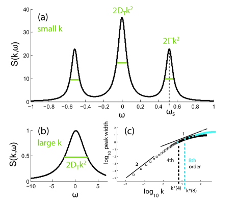
Figure 5: (a) Dynamic structure factor $S(k,\omega)$ vs. $\omega$ for a small $k=0.4$ and (b) large $k=100$. $\omega_{s}=c_{0}k$ denotes the hydrodnamics predicted sound mode of the spectrum, and the widths are related to the moments $A$–$Z$ (see Fig.  3). For small $k$, these are given by $D_{T}=\frac{2}{5}(X-Y)$ and $\Gamma=-(\frac{1}{2}A+\frac{1}{5}X+\frac{2}{15}Y)$, where $A$ is the generalized longitudinal kinetic viscosity, $Y$ the generalized thermal diffusion coefficient and $X$ is a cross-coupling transport coefficient, relating heat flux to density gradients. (c) Width $D_{T}k^{2}$ of the Rayleigh peak vs. $k$ (double-logarithmic). At small $k$, $D_{T}k^{2}\propto k^{2}$ as all moments $A$–$Z$, except $X$, reach a finite value in this limit. The inflection point at $k=k^{*}(N)\gg 1$ (shown to be increasing with the order of expansion $N$) denotes the onset of departure from the ideal Maxwellian behavior, where the width of the peak starts to behave sublinearly in $k$, and is used to quantify the range of validity for results obtained at finite order.

Representative plots of $S(k,\omega)$ are shown in Figs. 5a–b. For small $k$ (hydrodynamic limit), the spectrum we obtain recovers the usual results of neutron (or light) scattering experiments and consists of three Lorentzian peaks. The one centered in $\omega=0$ is the Rayleigh peak, which corresponds to the diffusive thermal mode. The two side peaks centered in $\omega\pm c_{0}k$ are the Brillouin peaks, and represent the two propagating sound waves. By increasing the wave-vector, the structure of (IV) is unchanged except that the generalized coefficients $D_{T}$ and $\Gamma$ need to be replaced by more complicate expressions, not given here. The net effect observed is that sound waves get strongly damped and vanish, whereas the central Rayleigh peak decreases and broadens. Density fluctuations are, therefore, driven only by a diffusive thermal mode for large enough $k$. A deeper look about the behavior of the width at half maximum of the central Rayleigh peak with increasing wavevectors allows us to bridge the gap between the hydrodynamic continuum-like description and the free particle limit. The hydrodynamic regime is featured by a width increasing with the square wavevector, $\propto k^{2}$. On the contrary, in the free particle limit, the calculation of the dynamical structure factor $S_{n,n}(k,\omega)$ reduces to the Fourier transform of the self part of the van Hove function $G_{s}(\textbf{r},t)$hansen , which, upon writing $\textbf{c}=\textbf{r}/t$, is given by the Maxwellian distribution: $G_{s}(\textbf{r},t)=\pi^{-3/2}v_{T}^{-3}t^{-3}\exp(-r^{2}/t^{2})$. Hence, the width of the peak is expected to grow up linearly in $k$, for large $k$. Our results, see Fig. 5c, predict a width which is truly quadratic for small enough $k$, reach the regime of linear behavior and terminate, for some large $k$, with a sub-linear dependence on $k$. The onset of the terminal regime at $k=k^{*}(N)$ marks the range of validity which can be accessed at a given finite order of expansion, $N$. Increasing $N$ thus does not alter the overall picture we obtained at a moderate order of expansion, and more generally, results obtained with $N+1$ will not change those obtained with $N$ below $k^{*}(N)$, cf. Fig. 5c.

V Conclusions

The main result of our paper is the characterization of the nonequilibrium distribution function, through the method of invariant manifolds, and the calculation of its moments (the functions $A$–$Z$), which constitute the building blocks of the generalized hydrodynamic equations. As we had previously shown in matteo2 , the latter equations are stable and hyperbolic for arbitrary wavevectors. Moreover, we have proposed and applied a route to solve the eigenvalue problem associated with the BE (6), by calculating the hydrodynamic modes, which we may regard either as decay rates of hydrodynamic fluctuations as well as generalized eigenfrequencies of the BE (3). The generalized transport coefficients have been numerically determined and settled into expressions recovering the Green-Kubo formulas. Finally, also by comparing with available experimental data and previous approaches, we discussed the range of validity of our approach, which turned out to be capable of extending the hydrodynamic scenario to length scales below the mean free path. This offers new perspectives towards a deeper comprehension of the transition between a “mesoscopic” particle-like description of matter and the “continuum” macroscopic one.

Acknowledgement

M.C. thanks Dr. I.V. Karlin for helpful discussions. This work was supported by EU-NSF contract NMP3-CT-2005- 016375 and FP6-2004-NMP-TI-4 STRP 033339 of the European Community

Appendix A Obtaining the invariance equation

In order to calculate the averages occurring in Sec. III, like $\langle\mu(\textbf{c})\rangle_{f}$, we switch to spherical coordinates. For each (at present arbitrary) wave vector $\textbf{k}=k{\bf e}_{\mbox{\tiny$\|$}}$, we choose the coordinate system in such a way that its (vertical) $z$-direction aligns with $\textbf{e}_{\mbox{\tiny$\|$}}$ and that its $x$–direction aligns with $\textbf{e}_{\mbox{\tiny$\bot$}}$. The velocity vector we had been decomposed earlier as $\tilde{\textbf{u}}=u^{\mbox{\tiny$\|$}}{\bf e}_{\mbox{\tiny$\|$}}+u^{\mbox{\tiny$\bot$}}{\bf e}_{\mbox{\tiny$\bot$}}$. We can then express c, over which we are going to perform all integrals, in terms of its norm $c$, a vertical variable $z$ and plane vector $\textbf{e}_{\phi}$ (azimuthal angle $\textbf{e}_{\phi}\cdot\textbf{e}_{\mbox{\tiny$\bot$}}=\cos\phi$; the plane contains ${\bf e}_{\mbox{\tiny$\bot$}}$) for the present purpose as:

$$\textbf{c}/c=\sqrt{1-z^{2}}\,\textbf{e}_{\phi}+z\textbf{e}_{\mbox{\tiny$\|$}},$$ (40)

as shown in Fig. 6.

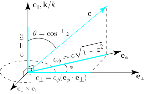
Figure 6: Schematic drawing introducing a orthonormal frame ${\bf e}_{\mbox{\tiny$\|$}}$, ${\bf e}_{\mbox{\tiny$\bot$}}$, and ${\bf e}_{\mbox{\tiny$\bot$}}\times{\bf e}_{\mbox{\tiny$\|$}}$ which is defined by the wavevector $\textbf{k}\,\|\,{\bf e}_{\mbox{\tiny$\|$}}$ and the heat flux ${\bf q}$ (not shown), which lies in the ${\bf e}_{\mbox{\tiny$\|$}}$–${\bf e}_{\mbox{\tiny$\bot$}}$–plane. Shown is the velocity vector ${\bf c}$ (40) relative to this frame (characterized by length $c$, coordinate $z$, and angle $\phi$) and its various components. The integration over $d^{3}c=c^{2}dcdzd\phi$ is done in spherical coordinates with respect to the local orthonormal basis.

The local Maxwellian, linearized around global equilibrium, takes the form: $f^{\textrm{LM}}/f^{\textrm{GM}}=1+\varphi_{0}=1+{\bf X}^{0}\cdot\textbf{x}$, where the four–dimensional ${\bf X}^{0}$, and the related vector $\xi$, employing four–dimensional $\textbf{x}=[\tilde{n},u^{\mbox{\tiny$\|$}},\tilde{T},u^{\mbox{\tiny$\bot$}}]$, are given by

$${\bf X}^{0}(\textbf{c}) = \left(1,2c_{\mbox{\tiny$\|$}},(c^{2}-\frac{3}{2}),2c_{\mbox{\tiny$\bot$}}\right),$$ (41a)

$$\mbox{\boldmath{$\xi$}}(\textbf{c}) = \left(1,c_{\mbox{\tiny$\|$}},\frac{2}{3}(c^{2}-\frac{3}{2}),c_{\mbox{\tiny$\bot$}}\right).$$ (41b)

Here, we introduced, for later use, the abbreviations

$$c_{\mbox{\tiny$\|$}}\equiv\textbf{c}\cdot\textbf{e}_{\mbox{\tiny$\|$}},\qquad c_{\mbox{\tiny$\bot$}}\equiv\textbf{c}\cdot\textbf{e}_{\mbox{\tiny$\bot$}},\qquad c_{\phi}\equiv{\bf c}\cdot\textbf{e}_{\phi}=\frac{c_{\mbox{\tiny$\bot$}}}{\textbf{e}_{\mbox{\tiny$\bot$}}\cdot\textbf{e}_{\phi}},$$ (42)

such that $i\textbf{k}\cdot\textbf{c}=ikc_{\mbox{\tiny$\|$}}$. We can then rewrite (40) as $\textbf{c}=c_{\phi}\textbf{e}_{\phi}+c_{\mbox{\tiny$\|$}}\textbf{e}_{\mbox{\tiny$\|$}}$ with $c_{\mbox{\tiny$\|$}}=cz$ and $c_{\phi}=c\sqrt{1-z^{2}}$. The latter two components, contrasted by $c_{\mbox{\tiny$\bot$}}$ (and $\textbf{e}_{\phi}$), do not depend on the azimuthal angle. We further introduced yet unknown fields $\delta{\bf X}({\bf c},\textbf{k})$ which characterize the nonequilibrium part of the distribution function, $\delta\varphi=\delta f/f^{\textrm{GM}}$. By analogy with the structure of the local Maxwellian, those are linear in terms of the hydrodynamic fields x themselves,

$$\delta\varphi=\delta{\bf X}\cdot\textbf{x}=\delta X_{1}\tilde{n}+\delta X_{2}u^{\mbox{\tiny$\|$}}+\delta X_{3}\tilde{T}+\delta X_{4}u^{\mbox{\tiny$\bot$}}.$$ (43)

The functions $\delta X_{1,2,3}$, which are associated to the longitudinal fields, inherit the full rotational symmetry of the corresponding Maxwellian components, $\delta X_{1,2,3}=\delta X_{1,2,3}(c,z)$, whereas $\delta X_{4}$ factorizes as $\delta X_{4}(c,z,\phi)=2\delta Y_{4}(c,z)\sum_{m=1}^{\infty}y_{m}\cos m\phi$. In this context it is an important technical aspect of our derivation to work with a suitable orthogonal set of basis functions (irreducible tensors, cf. irr , for models beyond the Maxwell gas) to represent $\delta f$ uniquely. The matrix ${\bf M}$ in (20) contains the non-hydrodynamic fields, the heat flux ${\bf q}\equiv\langle{\bf c}(c^{2}-\frac{5}{2})\rangle_{f}$ and the stress tensor $\mbox{\boldmath{$\sigma$}}\equiv\langle{\hskip 1.99997pt\stackrel{{\scriptstyle\vrule width=0.2411pt,height=0.2411pt,depth=1.43161pt\hbox{\vrule width=7.0622pt,height=0.2411pt,depth=0.0pt}\vrule width=0.2411pt,height=0.2411pt,depth=1.43161pt}}{{{\bf c}{\bf c}}}\hskip 1.99997pt}\rangle_{f}$, where ${\hskip 1.99997pt\stackrel{{\scriptstyle\vrule width=0.2411pt,height=0.2411pt,depth=1.43161pt\hbox{\vrule width=3.60107pt,height=0.2411pt,depth=0.0pt}\vrule width=0.2411pt,height=0.2411pt,depth=1.43161pt}}{{\bf s}}\hskip 1.99997pt}$ denotes the symmetric traceless part of a tensor ${\bf s}$ CKK12 ; tensorrechnung2 ; mkbook , ${\hskip 1.99997pt\stackrel{{\scriptstyle\vrule width=0.2411pt,height=0.2411pt,depth=1.43161pt\hbox{\vrule width=3.60107pt,height=0.2411pt,depth=0.0pt}\vrule width=0.2411pt,height=0.2411pt,depth=1.43161pt}}{{\bf s}}\hskip 1.99997pt}=\frac{1}{2}({\bf s}+{\bf s}^{T})-\frac{1}{3}{\rm tr}({\bf s})\mathbf{I}$. Using (16) and the above mentioned angular dependence of the $\delta{\bf X}$ functions (the only term in $\delta X_{4}$ playing a role in our calculations is the first order term $\cos\phi$, with $y_{1}=1$, see calc ), constraints, such as the required decoupling between longitudinal and transversal dynamics of the hydrodynamic fields, are automatically dealt with correctly when performing integrals over $\phi$. More explicitely calc , the stress tensor and heat flux uniquely decompose as follows

$$\sigma = \sigma^{\mbox{\tiny$\|$}}\,\frac{3}{2}{\hskip 1.99997pt\stackrel{{\scriptstyle\vrule width=0.2411pt,height=0.2411pt,depth=1.43161pt\hbox{\vrule width=11.0622pt,height=0.2411pt,depth=0.0pt}\vrule width=0.2411pt,height=0.2411pt,depth=1.43161pt}}{{{\bf e}_{\mbox{\tiny$\|$}}{\bf e}_{\mbox{\tiny$\|$}}}}\hskip 1.99997pt}+\sigma^{\mbox{\tiny$\bot$}}\,2{\hskip 1.99997pt\stackrel{{\scriptstyle\vrule width=0.2411pt,height=0.2411pt,depth=1.43161pt\hbox{\vrule width=12.17331pt,height=0.2411pt,depth=0.0pt}\vrule width=0.2411pt,height=0.2411pt,depth=1.43161pt}}{{{\bf e}_{\mbox{\tiny$\|$}}{\bf e}_{\mbox{\tiny$\bot$}}}}\hskip 1.99997pt},$$ (44a)

$${\bf q} = q^{\mbox{\tiny$\|$}}\,{\bf e}_{\mbox{\tiny$\|$}}+q^{\mbox{\tiny$\bot$}}\,{\bf e}_{\mbox{\tiny$\bot$}},$$ (44b)

with the moments $\sigma^{\mbox{\tiny$\|$}}=(\sigma^{\mbox{\tiny$\|$}}_{1},\sigma^{\mbox{\tiny$\|$}}_{2},\sigma^{\mbox{\tiny$\|$}}_{3})\cdot(\tilde{n},u^{\mbox{\tiny$\|$}},\tilde{T})$ and $\sigma^{\mbox{\tiny$\bot$}}=\sigma_{4}u^{\mbox{\tiny$\bot$}}$, and similarly for ${\bf q}$ (see Row 2 of Tab. 2). The prefactors arise from the identities ${\hskip 1.99997pt\stackrel{{\scriptstyle\vrule width=0.2411pt,height=0.2411pt,depth=1.43161pt\hbox{\vrule width=11.0622pt,height=0.2411pt,depth=0.0pt}\vrule width=0.2411pt,height=0.2411pt,depth=1.43161pt}}{{{\bf e}_{\mbox{\tiny$\|$}}{\bf e}_{\mbox{\tiny$\|$}}}}\hskip 1.99997pt}:{\hskip 1.99997pt\stackrel{{\scriptstyle\vrule width=0.2411pt,height=0.2411pt,depth=1.43161pt\hbox{\vrule width=11.0622pt,height=0.2411pt,depth=0.0pt}\vrule width=0.2411pt,height=0.2411pt,depth=1.43161pt}}{{{\bf e}_{\mbox{\tiny$\|$}}{\bf e}_{\mbox{\tiny$\|$}}}}\hskip 1.99997pt}=\frac{2}{3}$ and ${\hskip 1.99997pt\stackrel{{\scriptstyle\vrule width=0.2411pt,height=0.2411pt,depth=1.43161pt\hbox{\vrule width=12.17331pt,height=0.2411pt,depth=0.0pt}\vrule width=0.2411pt,height=0.2411pt,depth=1.43161pt}}{{{\bf e}_{\mbox{\tiny$\|$}}{\bf e}_{\mbox{\tiny$\bot$}}}}\hskip 1.99997pt}:{\hskip 1.99997pt\stackrel{{\scriptstyle\vrule width=0.2411pt,height=0.2411pt,depth=1.43161pt\hbox{\vrule width=12.17331pt,height=0.2411pt,depth=0.0pt}\vrule width=0.2411pt,height=0.2411pt,depth=1.43161pt}}{{{\bf e}_{\mbox{\tiny$\|$}}{\bf e}_{\mbox{\tiny$\bot$}}}}\hskip 1.99997pt}=\frac{1}{2}$. We note in passing that, while the stress tensor has, in general, three different eigenvalues, in the present symmetry adapted coordinate system it exhibits a vanishing first normal stress difference. Since the integral kernels of all moments in (44) do not depend on the azimuthal angle, these are actually two-dimensional integrals over $c\in[0,\infty]$ and $z\in[-1,1]$, each weighted by a component of $2\pi c^{2}f^{\textrm{GM}}\delta{\bf X}$. Stress tensor and heat flux can yet be written in an alternative form which is defined by Row 3 of Tab. 2. As we will prove below, due to fundamental symmetry considerations, the hereby introduced generalized transport coefficients $A$–$Z$ are real-valued. They can be expressed in terms of the moments of the distribution function, i.e., expansion coefficients ${\bf a}^{(r,l)}$, as follows:

$$A = -\frac{ia_{2}^{(0,2)}}{\sqrt{3}k},\quad B=-\frac{a_{1}^{(0,2)}}{\sqrt{3}k^{2}},$$

$$C = -\frac{a_{3}^{(0,2)}}{\sqrt{3}k^{2}},\quad X=-\frac{i\sqrt{5}a_{1}^{(1,1)}}{2k},$$

$$Y = -\frac{i\sqrt{5}a_{3}^{(1,1)}}{2k},\quad Z=-\frac{\sqrt{5}a_{2}^{(1,1)}}{2k^{2}},$$

$$D = -\frac{i}{k}\sum_{r,l}^{N}a_{4}^{(r,l)}\langle f^{\textrm{GM}}c_{\mbox{\tiny$\|$}}c_{\phi}|f^{\textrm{GM}}\Psi_{r,l}\rangle,$$

$$U = -\frac{1}{k^{2}}\sum_{r,l}^{N}a_{4}^{(r,l)}\langle f^{\textrm{GM}}(c^{2}-\frac{5}{2})c_{\phi}|f^{\textrm{GM}}\Psi_{r,l}\rangle.$$ (45)

We proceed by using these functions $A$–$Z$ to split ${\bf M}$ into parts as ${\bf M}={\rm Re}({\bf M})-i\,{\rm Im}({\bf M})$,

$${\bf M}=k^{2}\left(\begin{array}[]{cccc}0&0&0&0\\ 0&A&0&0\\ \frac{2}{3}X&0&\frac{2}{3}Y&0\\ 0&0&0&D\end{array}\right)-ik\left(\begin{array}[]{cccc}0&1&0&0\\ \tilde{B}&0&\tilde{C}&0\\ 0&\tilde{Z}&0&0\\ 0&0&0&0\end{array}\right),$$ (46)

with abbreviations $\tilde{B}\equiv\frac{1}{2}\!-\!k^{2}B$, $\tilde{C}\equiv\frac{1}{2}\!-\!k^{2}C$, and $\tilde{Z}\equiv\frac{2}{3}(1\!-\!k^{2}Z)$. The checkerboard structure of the matrix ${\bf M}$ (46) is particularly useful for studying properties of the hydrodynamic equations (20), such as hyperbolicity and stability (see CKK12 and below), once the functions $A$–$Z$ are explicitly evaluated. We remind the reader that we use orthogonal basis functions (irreducible moments, cf. Tab. 2) to solve (21). In order to show how the above functions enter the definition of the ${\bf M}$ matrix, we first notice that its elements are – a priori – complex valued. We wish, then, to make use of the fact that all integrals over $z$ vanish for odd integrands. To this end we introduce abbreviations $\oplus$ ($\ominus$) for a real-valued quantity which is even (odd) with respect to the transformation $z\rightarrow-z$. One notices ${\bf X}^{0}=(\oplus,\ominus,\oplus,\oplus)$, and we recall that $A$–$Z$ are integrals over either even or odd functions in $z$, times a component of $\delta{\bf X}$ (see Tab. 2).

Let us prove the consistency of the specified symmetry of M and the invariance condition: Start by assuming $A$–$Z$ to be real-valued functions. Then $M_{\mu\nu}=\oplus$ if $\mu+\nu$ is even, and $M_{\mu\nu}=i\oplus$ otherwise. This implies $\delta X_{1}=\oplus+i\ominus$, $\delta X_{2}=\ominus+i\oplus$, $\delta X_{3}=\oplus+i\ominus$, and $\delta X_{4}=\oplus+i\ominus$, i.e., different symmetry properties for real and imaginary parts. With these “symmetry” expressions for ${\bf X}^{0}$, $\delta{\bf X}$, and ${\bf M}$ at hand, and by noticing that symmetry properties for $\delta{\bf X}$ take over to $\hat{L}(\delta{\bf X})$ because the $\psi_{r,l}$ are (i) symmetric (antisymmetric) in $z$ for even (odd) $l$ and (ii) eigenfunctions of $\hat{L}$, we can insert into the right hand side of the equation, $\hat{L}(\delta{\bf X})=({\bf X}^{0}+\delta{\bf X})\cdot({\bf M}+i\ominus{\bf I})$, which is identical with the invariance equation (21). There are only two cases to consider, because ${\bf M}$ has a checkerboard structure, i.e., only two types of columns: Columns $\mu=1$ and $\mu=3$: $\delta X_{\mu}=\oplus+i\ominus$ because $M_{1-3,4}=0$; Columns $\mu\in\{2,4\}$: $\delta X_{\mu}=\oplus+i\ominus$ if $M_{\mu,1-3}=0$ (which is the case for column $4$) and $\ominus+i\oplus$ if $M_{\mu,4}=0$ (which is the case for column $2$). These observations complete the proof.

Appendix B Exact solution to the eigenvalue problem for a Maxwell-molecules collision operator

Given the linearized Boltzmann collision operator:

$$L\delta f = \int\int d\Omega d\textbf{c}_{1}\sigma(\Omega,g)gf^{\textrm{GM}}(c_{1})\times$$ (47)

$$[\delta\varphi(\textbf{k},\textbf{c})\!+\!\delta\varphi(\textbf{k},\textbf{c}_{1})\!-\!\delta\varphi(\textbf{k},\textbf{c}^{\prime})\!-\!\delta\varphi(\textbf{k},\textbf{c}_{1}^{\prime}]$$

where $g=|v-v_{1}|$ is the absolute value of the relative velocity and $\sigma(\Omega,g)$ the differential collision cross section. For so-called Maxwell molecules the collision probability per unit time is independent of the relative velocity:

$$g\sigma(\Omega,g)=\sqrt{\frac{2K(M+m)}{Mm}}F(\vartheta),$$ (48)

where $m$, $M$ are the masses of the colliding particles and $F(\vartheta)$, with $\vartheta\in[0,\pi]$, is given in parametric form through the parameter $\phi\in[0,\pi]$:

$$\vartheta(\phi) = \pi-2\sqrt{\cos(2\phi)}K(\sin\phi),$$ (49)

$$F(\vartheta) = \frac{[2^{3/2}\sin\vartheta\sin(2\phi)]^{-1}\sqrt{\cos 2\phi}}{\cos^{2}(\phi)K(\sin\phi)-\cos(2\phi)E(\sin\phi)},$$ (50)

with the elliptic integrals $K(x)=\int_{0}^{\pi/2}(1-x^{2}\sin^{2}y)^{-1/2}\,dy$, and $E(x)=\int_{0}^{\pi/2}(1-x^{2}\sin^{2}y)^{1/2}\,dy$. Since the collision operator is spherically symmetric in the velocity space, the dependence of the eigenfunctions upon the direction of c is expected to be spherically harmonic. Indeed, the eigenvalue problem admits the following solutions:

$$L[\psi_{r,l}(c,z)] = \lambda_{r,l}\psi_{r,l}(c,z),$$ (51)

$$\psi_{r,l}(c,z) = \sqrt{\frac{r!(l+\frac{1}{2})\sqrt{\pi}}{(l+r+\frac{1}{2})!}}\;c^{l}P_{l}(z)S_{l+\frac{1}{2}}^{(r)}(c^{2}),$$ (52)

where $S_{l+1/2}^{(r)}(x)$ are Sonine polynomials, and $P_{l}(z)$ are Legendre polynomials which act on the azimuthal component of the peculiar velocity ${\bf c}$. The Legendre and Sonine polynomials are each orthogonal sets,

$$\int_{-1}^{1}P_{l}(z)P_{n}(z)\,dz = \frac{2}{2l+1}\delta_{ln},$$

$$2\pi\int_{0}^{\infty}c^{2}e^{-c^{2}}c^{2l}S_{l+\frac{1}{2}}^{(r)}(c^{2})S_{l+\frac{1}{2}}^{(p)}(c^{2})\,dc = \frac{\pi(l+\frac{1}{2}+r)!}{r!}\delta_{rp}.$$

Accordingly, the $\psi_{r,l}$ are normalized to unity with the weight factor $f_{0}(c)=\pi^{-3/2}\exp(-c^{2})$ (as defined in Sec. II.1):

$$\delta_{rr^{\prime}}\delta_{ll^{\prime}} = 2\pi^{-1/2}\int_{-1}^{1}\!\int_{0}^{\infty}c^{2}e^{-c^{2}}\psi_{r,l}(c,z)\psi_{r^{\prime},l^{\prime}}(c,z)\,dcdz$$ (53)

$$\equiv \pi^{-3/2}\int e^{-c^{2}}\psi_{r,l}({\bf c})\psi_{r^{\prime},l^{\prime}}({\bf c})\,d^{3}c.$$

The corresponding eigenvalues for Maxwell molecules are given by:

$$\lambda_{r,l} = 2\pi\int\sin(\vartheta)F(\vartheta)T_{rl}(\vartheta)\,d\vartheta,$$ (54a)

$$T_{rl}(\vartheta) \equiv \cos^{2r+l}\left(\frac{\vartheta}{2}\right)P_{l}(\cos\frac{\vartheta}{2})+\sin^{2r+l}\left(\frac{\vartheta}{2}\right)P_{l}(\sin\frac{\vartheta}{2})$$ (54b)

$$-(1+\delta_{r0}\delta_{l0}),$$

The collision operator is negative semidefinite, that is, all eigenvalues are negative except $\lambda_{0,0}$, $\lambda_{0,1}$, and $\lambda_{1,0}$ which are zero and correspond to the collision invariants. As it was shown in uhlenbeck , there is no lower bound for the set of eigenvalues. Chang and Uhlenbeck’s investigation uhlenbeck of the dispersion of sound in a Maxwell molecules gas was based upon writing the deviation from the global equilibrium as: $(\varphi_{0}+\delta\varphi)=\sum_{\{r,l\}=0}^{\infty}a_{r,l}\Psi_{r,l}(\textbf{c})$ so that the eigenvalue equation reduces to an algebraic equation for the coefficients $a_{r,l}$:

$$\omega a_{r,l} = -i\textbf{k}\cdot\!\!\!\sum_{\{r^{\prime},l^{\prime}\}=0}^{\infty}\!\!\mbox{\boldmath{$\Omega$}}_{r,l,r^{\prime},l^{\prime}}a_{r^{\prime},l^{\prime}}+\lambda_{r,l}a_{r,l},$$ (55)

$$\mbox{\boldmath{$\Omega$}}_{r,l,r^{\prime},l^{\prime}} \equiv \langle f^{\textrm{GM}}\Psi_{r,l}|\textbf{c}|f^{\textrm{GM}}\Psi_{r^{\prime},l^{\prime}}\rangle.$$ (56)

The hydrodynamic modes for the Maxwell-molecules gas are found by setting to zero the determinant of the above system of linear equations. Within this approach, from the knowledge of the spectrum of $\hat{L}$, it is possible to solve the eigenvalue problem (3) for an arbitrary number of modes, just by tuning the number of eigenfunctions taken into account in the ansatz for the nonequilibrium distribution function. The peculiarity of the Maxwell-molecules gas lies in the fact that at any stage of approximation the modes recover and extend those corresponding to lower order approximations. This method produces results which are found to be in agreement with the CE expansion.

References

- (1) S. Chapman, T. G. Cowling, The Mathematical Theory of Nonuniform Gases (Cambridge Univ. Press, New York, 1970).
- (2) A.V. Bobylev, Sov. Phys. Dokl. 27, 29 (1982).
- (3) A.V. Bobylev, J. Stat. Phys. 124, 371 (2006).
- (4) A.N. Gorban, I.V. Karlin, Invariant Manifolds for Physical and Chemical Kinetics (Springer, Berlin, 2005).
- (5) L. Onsager, S. Machlup, Phys. Rev. 91, 1505 (1953).
- (6) P. Resibois, J. Stat. Phys. 2, No. 1 (1970).
- (7) J. M. Blatt, J. Phys. A: Math. Theor. 8, 980 (1975).
- (8) I.V. Karlin, M. Colangeli, M. Kröger, Phys. Rev. Lett. 100, 214503 (2008).
- (9) C.S. Wang Chang, G.E. Uhlenbeck, Stud. Stat. Mech. 5, 43 (1970).
- (10) A.V. Bobylev, I.M. Gamba, J. Stat. Phys. 124, 497 (2006).
- (11) M. Kröger, M. Hütter, J. Chem. Phys. 125, 044105 (2006).
- (12) W.E. Alley, B.J. Alder, Phys. Rev. A 27, 3158 (1983).
- (13) D. Forster, Hydrodynamic fluctuations, Broken Symmetry, and Corrrelation Functions (W. A. Benjamin, New York, 1975).
- (14) H. Struchtrup, M. Torrilhon, Phys. Rev. Lett. 99, 014502 (2007).
- (15) E. Meyer, G. Sessler, Z. Phys. 149, 15 (1957).
- (16) M. Colangeli, I.V. Karlin, M. Kröger, Phys. Rev. E 75, 051204 ; 76 (2007) 022201 (2007).
- (17) B.J. Alder, W.E. Alley, Phys. Today 37, 56 (1984).
- (18) H. Grad, “Principles of the kinetic theory of gases,” in Handbuch der Physik, edited by S. Flügge (Springer, Berlin, 1958), Vol. 12.
- (19) J.-P. Hansen, I.R. McDonald, Theory of Simple Liquids (Academic Press, 2006).
- (20) J.M. Ortiz De Zarate, J.V. Sengers, Hydrodynamic Fluctuations in Fluids and Fluid Mixtures (Elsevier, Amsterdam, 2006).
- (21) L.E. Reichl, A modern course in statistical physics, 2nd Ed. (John Wiley & Sons, New York, 1998).
- (22) M. Colangeli, I.V. Karlin, M. Kröger, Phys. Rev. E 76, 022201 (2007).
- (23) S. Hess, W. Köhler, Formeln zur Tensor-Rechnung (Palm & Enke, Erlangen, 1980).
- (24) M. Kröger, Models for Polymeric and Anisotropic Liquids (Springer, Berlin, 2005).
- (25) M. Abramowitz, I.A. Stegun, Handbook of mathematical functions (National Bureau of Standards, Washington, 1967).
- (26) Adopting the notation in tensorrechnung2 ; mkbook the distribution function is written as a sum over –fold contracted products of th rank tensors, with and base functions , where are the associated Laguerre (th order) polynomials abramowitz , denotes the –fold tensor product, and denotes the irreducible part of a tensor a. For the explicit construction of th rank irreducible tensors see page 160 of mkbook . The normalization coefficients evaluate as . The base function is thus a th order polynomial in . The lowest order base functions read , , , , and . Density, velocity, temperature, heat flux, and stress tensor are related to the moments as follows: , , , , and . The distribution function is then split into (orthogonal) parts as with and , while the sum in extends over the remaining –pairs. Density, velocity, and temperature are therefore determined by alone, and automatically obeys constrains such as orthogonality requirement and also , as mentioned in the text part. These conditions become redundant ones calculations are performed using the particular basis . For Maxwell molecules, the dependence on the polar angle can be included by replacing by involving the associated Legendre polynomials abramowitz , and the eigenvalues are independent of . Then, these base function reduce to the eigenfunctions (52) of the Maxwell gas .
-
(27)
The integrals listed
in Tab. 2 obey the following decoupling rules:
(39)