Multi-User Diversity vs. Accurate Channel State Information in MIMO Downlink Channels

Abstract

In a multiple transmit antenna, single antenna per receiver downlink channel with limited channel state feedback, we consider the following question: given a constraint on the total system-wide feedback load, is it preferable to get low-rate/coarse channel feedback from a large number of receivers or high-rate/high-quality feedback from a smaller number of receivers? Acquiring feedback from many receivers allows multi-user diversity to be exploited, while high-rate feedback allows for very precise selection of beamforming directions. We show that there is a strong preference for obtaining high-quality feedback, and that obtaining near-perfect channel information from as many receivers as possible provides a significantly larger sum rate than collecting a few feedback bits from a large number of users.

I Introduction

Multi-user multiple-input, multiple-output (MU-MIMO) communication is very powerful and has recently been the subject of intense research. A transmitter equipped with $N_{t}$ antennas can serve up to $N_{t}$ users simultaneously over the same time-frequency resource, even if each receiver has only a single antenna. Such a model is very relevant to many applications, such as the cellular downlink from base station (BS) to mobiles (users). However, knowledge of the channel is required at the BS in order to fully exploit the gains offered by MU-MIMO.

In systems without channel reciprocity (such as frequency-division duplexed systems), the BS obtains Channel State Information (CSI) via channel feedback from mobiles. In the single antenna per mobile setting, feedback strategies involve each mobile quantizing its $N_{t}$-dimensional channel vector and feeding back the corresponding bits approximately every channel coherence time. Although there has been considerable prior work on this issue of channel feedback, e.g., optimizing feedback contents and quantifying the sensitivity of system throughput to the feedback load, almost all of it has been performed from the perspective of the per-user feedback load. Given that channel feedback consumes considerable uplink resources (bandwidth and power), the aggregate feedback load, summed across users, is more meaningful than the per-user load from a system design perspective. However, it is not yet well understood how an aggregate feedback budget is best utilized.

Thereby motivated, in this paper we ask the following fundamental design question:
For a fixed aggregate feedback load, is a larger system sum rate achieved by collecting a small amount of per-user feedback from a large number of users, or by collecting a larger amount of per-user feedback from a smaller subset of users?

Assuming an aggregate feedback load of $T_{\text{fb}}$ bits, we consider a system where $T_{\text{fb}}/B$ users quantize their channel direction to $B$ bits each and feed back these bits along with one real number (per user) representing the channel quality. The BS then selects, based upon the feedback received from the $T_{\text{fb}}/B$ users, up to $N_{t}$ users for transmission using multi-user beamforming. A larger value of $B$ corresponds to more accurate CSI but fewer users and reduced multi-user diversity. By comparing the sum rates for different values of $B$, we reach the following simple but striking conclusion: for almost any number of antennas $N_{t}$, average SNR, and feedback budget $T_{\text{fb}}$, sum rate is maximized by choosing $B$ (feedback bits per user) such that near-perfect CSI is obtained for each of the $T_{\text{fb}}/B$ users that do feedback. In other words, accurate CSI is more valuable than multi-user diversity.

In a 4 antenna ($N_{t}=4$) system operating at 10 dB with $T_{\text{fb}}=100$ bits, for example, it is near-optimal to have $5$ users (arbitrarily chosen from a larger user set) feed back $B=20$ bits each. This provides a sum rate of $9.9$ bps/Hz, whereas $10$ users with $B=10$ with and $25$ users with $B=4$ (i.e., operating with less accurate CSI ) provide sum rates of only $8.5$ and $4.6$, respectively.

Our finding is rather surprising in the context of prior work on schemes with a very small per-user feedback load. Random beamforming (RBF), which requires only $\log_{2}N_{t}$ feedback bits per user, achieves a sum rate that scales with the number of users in the same manner as the perfect-CSI sum rate [1], and thus appears to be a good technique when there are a large number of users. On the contrary, we find that RBF achieves a significantly smaller sum rate than a system using a large value of $B$. This is true even when $T_{\text{fb}}$ is extremely large, in which case the number of users who feedback is very large (and thus multi-user diversity is plentiful) if RBF is used.

Although perhaps not initially apparent, the problem considered here has very direct relevance to system design. The designer must specify how often (in time) mobiles feed back CSI and the portion of the channel response (in frequency) that the CSI feedback corresponds to. If each mobile feeds back CSI for essentially every time/frequency coherence block, then the BS will have many users to select from (on every block) but, assuming a constraint on the total feedback, the CSI accuracy will be rather limited, thereby corresponding to a small value of $B$ in our setup. On the other hand, mobiles could be grouped in frequency and/or time and thus only feed back information about a subset of time/frequency coherence blocks; this corresponds to fewer users but more accurate CSI (i.e., larger $B$) on each resource block. Our results imply a very strong preference towards the latter strategy.

The remainder of the paper is organized as follows. In Section II we discuss related prior work, while in Section III we describe the system model and the different beamforming/feedback techniques (zero-forcing, RBF, and its extension PU²RC). In Section IV we determine the optimal value of $B$ for zero-forcing (ZF) and characterize the dependence of the optimizer on $N_{t}$, SNR, and $T_{\text{fb}}$. In Section V we perform the same optimization for PU²RC. In Section VI we compare ZF and RBF/PU²RC and illustrate the large sum rate advantage of ZF (with large $B$), while in Section VII we see that our basic conclusion is upheld even if low complexity user selection and quantization is performed, as well as if the channel feedback is delayed. Because much of the work is based on numerical results, the associated MATLAB code has been made available online [2].

II Related Work

Perhaps the most closely related work is [3], where the tradeoff between multi-user diversity and accurate CSI is studied in the context of two-stage feedback. In the first stage all users feed back coarse estimates of their channel, based on which the transmitter runs a selection algorithm to select $N_{t}$ users who feed back more accurate channel quantization during the second feedback stage, and the split of the feedback budget between the two stages is optimized. Our work differs in that we consider only a single stage approach, and more importantly in that we optimize the number of users (randomly selected) who feed back accurate information rather than limiting this number to $N_{t}$. Indeed, this optimization is precisely why our approach shows such large gains over simple RBF or un-optimized ZF.

There has also been related work on systems with channel-dependent feedback, in which each user determines whether or not to feed back on the basis of its current channel condition (i.e., channel norm and quantization error) [4][5][6][7][8]. As a result, the BS does not a priori know who feeds back and thus there is a random-access component to the feedback. Channel-dependent feedback intuitively appears to provide an advantage because only users with good channels feed back. Although some of this prior work has considered aggregate feedback load (c.f., [9]), that work has not considered optimization of $B$, the per-user feedback load, as we do here for channel-independent feedback. We are currently investigating the per-user optimization for channel-dependent feedback and our preliminary results in fact reinforce the basic conclusions of the present work. However, this is beyond the scope of this paper and we consider only channel-independent feedback here (meaning the users who do feed back are arbitrary in terms of their channel conditions).

III System Model & Background

We consider a multi-input multi-output (MIMO) Gaussian broadcast channel in which the Base Station (the BS or transmitter) has $N_{t}$ antennas and each of the users or User Terminals (the UT, mobile or receiver) have 1 antenna each (Figure 1). The channel output $y_{k}$ at user $k$ is given by:

$$y_{k}={\bf h}_{k}^{\sf H}{\bf x}+z_{k},\;\;k=1,\ldots,K$$ (1)

where $z_{k}\sim{\cal C}{\cal N}(0,1)$ models Additive White Gaussian Noise (AWGN), ${\bf h}_{k}\in\mbox{\bb C}^{N_{t}}$ is the vector of channel coefficients from the $k^{\textrm{th}}$ user antenna to the transmitter antenna array and ${\bf x}$ is the vector of channel input symbols transmitted by the base station. The channel input is subject to an average power constraint $\mbox{\bb E}\left[||{\bf x}||_{2}^{2}\right]\leq\mbox{\scriptsize\sf SNR}$. We assume that the channel state, given by the collection of all channel vectors, varies in time according to a block-fading model, where the channels are constant within a block but vary independently from block to block. The entries of each channel vector are i.i.d. Gaussian with elements $\sim{\cal C}{\cal N}(0,1)$. Each user is assumed to know its own channel perfectly.

At the beginning of each block, each user quantizes its channel to $B$ bits and feeds back the bits, in an error- and delay-free manner, to the BS (see Figure 1). Vector quantization is performed using a codebook ${\mathcal{C}}$ that consists of $2^{B}$ $N_{t}$-dimensional unit norm vectors ${\mathcal{C}}\triangleq\{\mathbf{w}_{1},\ldots,\mathbf{w}_{2^{B}}\}$. Each user quantizes its channel vector to the quantization vector that forms the minimum angle to it. Thus, user $k$ quantizes its channel to $\widehat{{\bf h}}_{k}$ and feeds the $B$-bit index back to the transmitter, where $\widehat{{\bf h}}_{k}$ is chosen according to:

$$\widehat{{\bf h}}_{k} = \textrm{arg}\min_{{\bf w}\in\ {\mathcal{C}}}\ \sin^{2}\left(\angle({\bf h}_{k},{\bf w})\right).$$ (2)

where $\cos^{2}\left(\angle({\bf h}_{k},{\bf w})\right)=\frac{|{\bf h}_{k}^{\sf H}{\bf w}|^{2}}{||{\bf h}_{k}||^{2}||{\bf w}_{k}||^{2}}=1-\sin^{2}\left(\angle({\bf h}_{k},{\bf w})\right)$. The specifics of the quantization codebook are discussed later. Each user also feeds back a single real number, which can be the channel norm or some other Channel Quality Indicator (CQI). We assume that this CQI is known perfectly to the BS, i.e., it is not quantized, and thus CQI feedback is not included in the feedback budget; this simplification is investigated in Section VII-D.

For a total aggregate feedback load of $T_{\text{fb}}$ bits, we are interested in the sum rate (of the different feedback/beamforming strategies described later in this section) when $T_{\text{fb}}/B$ users feed back $B$ bits each. The $T_{\text{fb}}/B$ users who feed back are arbitrarily selected from a larger user set. Furthermore, in our block fading setting, only those users who feed back in a particular block/coherence time are considered for transmission in that block; in other words, we are limited to transmitting to a subset of only the $T_{\text{fb}}/B$ users.

III-A Zero Forcing Beamforming

When Zero-Forcing (ZF) is used, each user feeds back the $B$-bit quantization of its channel direction as well as the channel norm $||{\bf h}_{k}||$ representing the channel quality (different channel quality indicator (CQI) choices are considered in Section VII-A). The BS then uses the greedy user selection algorithm described in [10], adopted to imperfect CSI by treating the vector $||{\bf h}_{k}||\cdot\widehat{{\bf h}}_{k}$ (which is known to the BS) as if it were user $k$’s true channel. The algorithm first selects the user with the largest CQI. In the next step the ZF sum rate is computed for every pair of users that includes the first selected user (where the rate is computed assuming $||{\bf h}_{k}||\cdot\widehat{{\bf h}}_{k}$ is the true channel of user $k$), and the additional user that corresponds to the largest sum rate is selected next. This process of adding one user at a time, in greedy fashion, is continued until $N_{t}$ users are selected or there is no increase in sum rate. Unlike [10], we do not optimize power and instead equally split power amongst the selected users.

We denote the indices of selected users by $\Pi(1),\ldots,\Pi(n)$, where $n\leq N_{t}$ is the number of users selected ($n$ depends on the particular channel vectors). By the ZF criterion, the unit-norm beamforming vector $\widehat{{\bf v}}_{\Pi(k)}$ for user $\Pi(k)$ is chosen in the direction of the projection of $\widehat{{\bf h}}_{\Pi(k)}$ on the nullspace of $\{\widehat{{\bf h}}_{\Pi(j)}\}_{j\neq k}$. Although ZF beamforming is used, there is residual interference because the beamformers are based on imperfect CSI. The (post-selection) SINR for selected user $\Pi(k)$ is

$$\mbox{\scriptsize\sf SINR}_{\Pi(k)}=\frac{\frac{\mbox{\scriptsize\sf SNR}}{n}||{\bf h}_{\Pi(k)}||^{2}\cos^{2}\left(\angle({\bf h}_{\Pi(k)},\widehat{{\bf v}}_{\Pi(k)})\right)}{1+\frac{\mbox{\scriptsize\sf SNR}}{n}||{\bf h}_{\Pi(k)}||^{2}\sum\limits_{j\neq k}\cos^{2}\left(\angle({\bf h}_{\Pi(k)},\widehat{{\bf v}}_{\Pi(j)})\right)},$$ (3)

and the corresponding sum rate is $\sum_{k=1}^{n}\log_{2}(1+\mbox{\scriptsize\sf SINR}_{\Pi(k)})$.

For the sake of analysis and ease of simulation, each user utilizes a quantization codebook ${\mathcal{C}}$ consisting of unit-vectors independently chosen from the isotropic distribution on the $N_{t}$-dimensional unit sphere [11] (Random Vector Quantization or RVQ). Each user’s codebook is independently generated, and sum rate is averaged over this ensemble of quantization codebooks. Although we focus on RVQ, in Section VII-C we show that our conclusions are not dependent on the particular quantization scheme used.

In [13] it is shown that the sum rate of ZF beamforming with quantized CSI but without user selection (i.e. $N_{t}$ users are randomly selected) is lower bounded by:

$$R^{\text{CSI}}_{\text{ZF-no selection}}(\mbox{\scriptsize\sf SNR})-N_{t}\log_{2}\left(1+\mbox{\scriptsize\sf SNR}\cdot 2^{-\frac{B}{N_{t}-1}}\right).$$ (4)

where $R^{\text{CSI}}_{\text{ZF-no selection}}(\mbox{\scriptsize\sf SNR})$ is the perfect CSI rate. This bound, which is quite accurate for large values of $B$ [13], indicates that ZF beamforming is very sensitive to the CSI accuracy. With $N_{t}=4$ and $\mbox{\scriptsize\sf SNR}=10$ dB, for example, $B=10$ corresponds to a sum rate loss of $4$ bps/Hz (relative to perfect CSI) and $17$ bits are required to reduce this loss to $1$ bps/Hz. Equation 4 is no longer a lower bound when user selection is introduced, but nonetheless it is a reasonable approximation and hints at the importance of accurate CSI.

III-B Random Beamforming

Random beamforming (RBF) was proposed in [1][14], wherein each user feeds back $\log_{2}N_{t}$ bits along with one real number. In this case, there is a common quantization codebook ${\mathcal{C}}$ consisting of $N_{t}$ orthogonal unit vectors and quantization is performed according to (2). In addition to the quantization index, each user feeds back a real number representing its SINR. If ${\bf w}_{m}$ ($1\leq m\leq N_{t}$) is the selected quantization vector for user $k$, then

$$\mbox{\scriptsize\sf SINR}_{k}=\frac{\frac{\mbox{\scriptsize\sf SNR}}{N_{t}}|{\bf h}_{k}^{\sf H}{\bf w}_{m}|^{2}}{1+\frac{\mbox{\scriptsize\sf SNR}}{N_{t}}\sum\limits_{n\neq m}|{\bf h}_{k}^{\sf H}{\bf w}_{n}|^{2}}=\frac{||{\bf h}_{k}||^{2}\cos^{2}\left(\angle{{\bf h}_{k},{\bf w}_{m}}\right)}{\frac{N_{t}}{\mbox{\scriptsize\sf SNR}}+||{\bf h}_{k}||^{2}\sin^{2}\left(\angle{{\bf h}_{k},{\bf w}_{m}}\right)}.$$ (5)

After receiving the feedback, the BS selects the user with the largest SINR on each of the $N_{t}$ beams $({\bf w}_{1},\dots,{\bf w}_{N_{t}})$, and beamforming is performed along these same vectors.

III-C PU²RC

Per unitary basis stream user and rate control ($\text{PU}^{2}\text{RC}$), proposed in [15] (a more widely available description can be found in [4]), is a generalization of RBF in which there is a common quantization codebook ${\mathcal{C}}$ consisting of $2^{B-\log_{2}N_{t}}$ ‘sets’ of orthogonal codebooks, where each orthogonal codebook consists of $N_{t}$ orthogonal unit vectors, and thus a total of $2^{B}$ vectors. Quantization is again performed according to (2), and each user feeds back the same SINR statistic as in RBF. User selection is performed as follows: for each of the orthogonal sets the BS repeats the RBF user selection procedure and computes the sum rate (where the per-user rate is $\log_{2}(1+\mbox{\scriptsize\sf SINR})$), after which it selects the orthogonal set with the highest sum rate. If $B=\log_{2}N_{t}$, there is only a single orthogonal set and the scheme reduces to ordinary RBF.

The primary difference between PU²RC and ZF is the user selection algorithm: $\text{PU}^{2}\text{RC}$ is restricted to selecting users within one of the orthogonal sets and thus has very low complexity, whereas the described ZF technique has no such restriction.

IV Optimization of Zero-Forcing Beamforming

Let $R_{\textsc{ZF}}\left(\mbox{\scriptsize\sf SNR},N_{t},\frac{T_{\text{fb}}}{B},B\right)$ be the sum rate for a system using ZF with $N_{t}$ antennas at the transmitter, signal-to-noise ratio SNR, and $\frac{T_{\text{fb}}}{B}$ users each feeding back $B$ bits. From Section III-A, we have:

$$R_{\textsc{ZF}}\left(\mbox{\scriptsize\sf SNR},N_{t},\frac{T_{\text{fb}}}{B},B\right) = \mbox{\bb E}\left[\sum\limits_{k=1}^{n}\log_{2}\left(1+\frac{\frac{\mbox{\scriptsize\sf SNR}}{n}||{\bf h}_{\Pi(k)}||^{2}\cos^{2}\left(\angle({\bf h}_{\Pi(k)},\widehat{{\bf v}}_{\Pi(k)})\right)}{1+\frac{\mbox{\scriptsize\sf SNR}}{n}||{\bf h}_{\Pi(k)}||^{2}\sum\limits_{j\neq k}\cos^{2}\left(\angle({\bf h}_{\Pi(k)},\widehat{{\bf v}}_{\Pi(j)})\right)}\right)\right]~{}$$ (6)

No closed form for this expression is known to exist, even in the case of perfect CSI, but this quantity can be easily computed via Monte Carlo simulation. We are interested in the number of feedback bits per user $B_{\textsc{ZF}}^{\textsc{OPT}}\left(\mbox{\scriptsize\sf SNR},N_{t},T_{\text{fb}}\right)$ that maximizes this sum rate for a total feedback budget of $T_{\text{fb}}$:

$$B_{\textsc{ZF}}^{\textsc{OPT}}\left(\mbox{\scriptsize\sf SNR},N_{t},T_{\text{fb}}\right) \triangleq \mathop{\rm argmax}_{\log_{2}N_{t}\leq B\leq\frac{T_{\text{fb}}}{N_{t}}}\ R_{\textsc{ZF}}\left(\mbox{\scriptsize\sf SNR},N_{t},\frac{T_{\text{fb}}}{B},B\right).$$ (7)

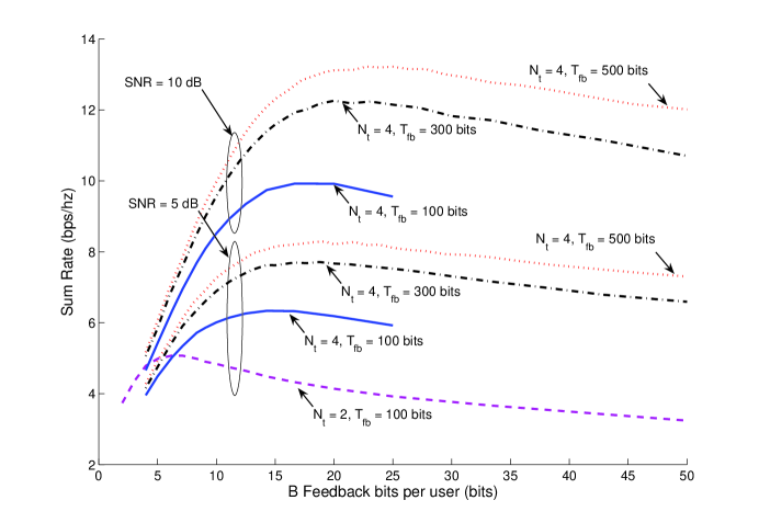
Figure 2: Sum rate Vs. Feedback load for Zero-forcing

Although this optimization is not tractable, it is well-behaved and can be meaningfully understood. Consider first Figure 2, where the sum rate $R_{\textsc{ZF}}\left(\mbox{\scriptsize\sf SNR},N_{t},\frac{T_{\text{fb}}}{B},B\right)$ is plotted versus $B$ for $2$ and $4$-antenna systems for various values of SNR and $T_{\text{fb}}$. Based on this plot it is immediately evident that the sum rate increases very rapidly with $B$, and that the rate-maximizing $B_{\textsc{ZF}}^{\textsc{OPT}}$ is very large, e.g., in the range $15-20$ and $20-25$ for $N_{t}=4$ at $5$ and $10$ dB, respectively. Both of these observations indicate a strong preference for accurate CSI over multi-user diversity.

In order to understand this behavior, we introduce the sum rate approximation

$$\widetilde{R}_{\textsc{ZF}}\left(\mbox{\scriptsize\sf SNR},N_{t},\frac{T_{\text{fb}}}{B},B\right) \triangleq N_{t}\ \log_{2}\left[1+\frac{\left(\frac{\mbox{\scriptsize\sf SNR}}{N_{t}}\right)\log\left(\frac{T_{\text{fb}}N_{t}}{B}\right)}{1+\left(\frac{\mbox{\scriptsize\sf SNR}}{N_{t}}\right)2^{-\frac{B}{N_{t}-1}}\log\left(\frac{T_{\text{fb}}N_{t}}{B}\right)}\right],$$ (8)

with $R_{\textsc{ZF}}\approx\widetilde{R}_{\textsc{ZF}}$. This approximation is obtained from the expression for $R_{\textsc{ZF}}$ in (6) by (a) replacing $||{\bf h}_{\Pi(k)}||^{2}$ with $\log\left(\frac{T_{\text{fb}}N_{t}}{B}\right)$, the expectation of the largest channel norm among $\frac{T_{\text{fb}}}{B}$ users from (33) in Appendix A, (b) assuming that the maximum number of users are selected (i.e., $n=N_{t}$), (c) replacing each $\cos^{2}\left(\angle({\bf h}_{\Pi(k)},\widehat{{\bf v}}_{\Pi(j)})\right)$ in the SINR denominator with its expected value $2^{-\frac{B}{N_{t}-1}}/(N_{t}-1)$ [13, Lemma 2], and (d) approximating the $\cos^{2}\left(\angle({\bf h}_{\Pi(k)},\widehat{{\bf v}}_{\Pi(k)})\right)$ term in the SINR numerator with unity.

In (8) the received signal power is $\left(\mbox{\scriptsize\sf SNR}/N_{t}\right)\log\left(T_{\text{fb}}N_{t}/B\right)$, while the interference power is $2^{-\frac{B}{N_{t}-1}}$ times the signal power. Imperfect CSI is evidenced in the $2^{-\frac{B}{N_{t}-1}}$ term in the interference power, while multi-user diversity is reflected in the $\log\left(T_{\text{fb}}N_{t}/B\right)$ term. Although not exact, the approximation in (8) is reasonably accurate and captures many key elements of the problem at hand.

We first use the approximation to explain the rapid sum rate increase with $B$. From (8) we see that increasing $B$ by $N_{t}-1$ bits reduces the interference power by a factor of $2$. As long as the interference power is significantly larger than the noise power, this leads to (approximately) a $3$ dB SINR increase and thus a $N_{t}$ bps/Hz sum rate increase. Dropping the two instances of $1$ in (8) crudely gives:

$$\widetilde{R}_{\textsc{ZF}}\left(\mbox{\scriptsize\sf SNR},N_{t},\frac{T_{\text{fb}}}{B},B\right) \approx \frac{N_{t}}{N_{t}-1}B.$$ (9)

Hence, sum rate increases almost linearly with $B$ when $B$ is not too large, consistent with Fig. 2. This discussion has neglected the fact that increasing $B$ comes at the expense of decreasing the number of users who feedback, thereby decreasing multi-user diversity. However, the accompanying decrease in sum rate is essentially negligible because (a) $\log\left(T_{\text{fb}}N_{t}/B\right)$ is only mildly decreasing in $B$ due to the nature of the logarithm, and (b) both signal and interference power are reduced by the same factor.

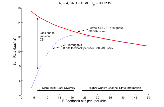
Figure 3: Sum rate Vs. Feedback load for Zero-forcing

It is clear that accurate CSI (i.e., a larger value of $B$) is strongly preferred to multi-user diversity in the range of $B$ for which sum rate increases roughly linearly with $B$. However, from Figure 2 we see that this linear scaling runs out and that a peak is eventually reached, beyond which increasing $B$ actually decreases sum rate. To understand the desired combination of CSI and multi-user diversity at $B_{\textsc{ZF}}^{\textsc{OPT}}$, in Figure 3 the sum rate $R_{\textsc{ZF}}\left(\mbox{\scriptsize\sf SNR},N_{t},\frac{T_{\text{fb}}}{B},B\right)$ as well as the perfect CSI sum rate for the same number of users (i.e., $\frac{T_{\text{fb}}}{B}$ users) $R_{\textsc{ZF}}\left(\mbox{\scriptsize\sf SNR},N_{t},\frac{T_{\text{fb}}}{B},\infty\right)$ are plotted versus $B$ for a system with $N_{t}=4$, $T_{\text{fb}}=300$ bits and $\mbox{\scriptsize\sf SNR}=10$ dB. Motivated by [13, Theorem 1] (see Section III-A for discussion), we approximate the sum rate by the perfect CSI sum rate minus a multi-user interference penalty term:

$$R_{\textsc{ZF}}\left(\mbox{\scriptsize\sf SNR},N_{t},\frac{T_{\text{fb}}}{B},B\right) \approx R_{\textsc{ZF}}\left(\mbox{\scriptsize\sf SNR},N_{t},\frac{T_{\text{fb}}}{B},\infty\right)-N_{t}\ \log_{2}\left(1+\frac{\mbox{\scriptsize\sf SNR}}{N_{t}}2^{-\frac{B}{N_{t}-1}}\log\frac{T_{\text{fb}}N_{t}}{B}\right)$$ (10)

This penalty term reasonably approximates the loss due to imperfect CSI which is indicated in Figure 3. In the figure we see that for $B\geq 25$ the sum rate curves for perfect and imperfect CSI essentially match and thus the penalty term in (10) is nearly zero. As a result, it clearly does not make sense to increase $B$ beyond $25$ because doing so reduces the number of users but does not provide a measurable CSI benefit. Keeping this in mind, the most interesting observation gleaned from Figure 3 is that $B_{\textsc{ZF}}^{\textsc{OPT}}$ corresponds to a point where the loss due to imperfect CSI is very small. In other words, it is optimal to operate at the point where effectively the maximum benefit of accurate CSI has been reaped.

At this point it is worthwhile to reconsider the sum rate versus $B$ curves in Figure 2. Although $B_{\textsc{ZF}}^{\textsc{OPT}}$ is quite large for all parameter choices, it is not particularly dependent on the total feedback budget $T_{\text{fb}}$. On the other hand, $B_{\textsc{ZF}}^{\textsc{OPT}}$ does appear to be increasing in SNR and $N_{t}$, and also seems quite sensitive to these parameters. To grasp these points and to develop a more quantitative understanding of the optimal $B$, we return to the approximation in (8). The optimal $B$ corresponding to this approximation is:

$$B_{\textsc{ZF}}^{\textsc{OPT}}\left(\mbox{\scriptsize\sf SNR},N_{t},T_{\text{fb}}\right) \approx \widetilde{B}_{\textsc{ZF}}^{\textsc{OPT}}\left(\mbox{\scriptsize\sf SNR},N_{t},T_{\text{fb}}\right)\ \triangleq\mathop{\rm argmax}_{\log_{2}N_{t}\leq B\leq\frac{T_{\text{fb}}}{N_{t}}}\ \widetilde{R}_{\textsc{ZF}}\left(\mbox{\scriptsize\sf SNR},N_{t},\frac{T_{\text{fb}}}{B},B\right).$$

The approximation is concave in $B$, and thus the following fixed point characterization of $\widetilde{B}_{\textsc{ZF}}^{\textsc{OPT}}$ is obtained by setting the derivative of $\widetilde{R}_{\textsc{ZF}}\left(\mbox{\scriptsize\sf SNR},N_{t},\frac{T_{\text{fb}}}{B},B\right)$ to zero:

$$\frac{\mbox{\scriptsize\sf SNR}}{N_{t}}2^{-\frac{\widetilde{B}_{\text{ZF}}^{\textsc{OPT}}}{N_{t}-1}}\frac{\widetilde{B}_{\text{ZF}}^{\textsc{OPT}}\log 2}{N_{t}-1}\left(\log\frac{T_{\text{fb}}N_{t}}{\widetilde{B}_{\text{ZF}}^{\textsc{OPT}}}\right)^{2}=1.$$ (11)

This quantity is easily computed numerically, but a more analytically convenient form is found as follows. By defining

$$L\triangleq\left(\log\frac{T_{\text{fb}}N_{t}}{\widetilde{B}_{\text{ZF}}^{\textsc{OPT}}\left(\mbox{\scriptsize\sf SNR},N_{t},T_{\text{fb}}\right)}\right)^{2}$$ (12)

and appropriately substituting, (11) can be rewritten in the following form:

$$\widetilde{B}_{\text{ZF}}^{\textsc{OPT}}\left(\mbox{\scriptsize\sf SNR},N_{t},T_{\text{fb}}\right) = -\frac{N_{t}-1}{\log 2}\ W_{-1}\left(-\frac{N_{t}}{\mbox{\scriptsize\sf SNR}}\frac{1}{L}\right)$$ (13)

where $W_{-1}(\cdot)$ is branch -1 of the LambertW function [16]. From [16, Equation 4.19], the following asymptotic expansion of $W_{-1}(-x)$ holds for small $x>0$:

$$W_{-1}(-x)=\log(x)+\log\left(\log\frac{1}{x}\right)+O\left(\frac{\log\left(\log\frac{1}{x}\right)}{\log(x)}\right).$$ (14)

Using (14) in (13), we have the following asymptotic expansion for $\widetilde{B}_{\text{ZF}}^{\textsc{OPT}}\left(\mbox{\scriptsize\sf SNR},N_{t},T_{\text{fb}}\right)$:

$$\widetilde{B}_{\text{ZF}}^{\textsc{OPT}}\left(\mbox{\scriptsize\sf SNR},N_{t},T_{\text{fb}}\right) \sim (N_{t}-1)\log_{2}\frac{\mbox{\scriptsize\sf SNR}}{N_{t}}+(N_{t}-1)\log_{2}\frac{L}{N_{t}}+(N_{t}-1)\log_{2}\left(\log\frac{\mbox{\scriptsize\sf SNR}}{N_{t}}L\right)$$ (15)

By repeatedly applying the asymptotic expansion of $W_{-1}(\cdot)$ to the occurrences of $L$ in (15), we can expand $\widetilde{B}_{\text{ZF}}^{\textsc{OPT}}\left(\mbox{\scriptsize\sf SNR},N_{t},T_{\text{fb}}\right)$ as a function of $T_{\text{fb}},\mbox{\scriptsize\sf SNR}$ and $N_{t}$ to yield the following:

$$\widetilde{B}_{\text{ZF}}^{\textsc{OPT}}\left(\mbox{\scriptsize\sf SNR},N_{t},T_{\text{fb}}\right) \mathop{\sim}\limits^{\text{Large}\ T_{\text{fb}}} O(\log\log T_{\text{fb}})$$ (16)

$$\widetilde{B}_{\text{ZF}}^{\textsc{OPT}}\left(\mbox{\scriptsize\sf SNR},N_{t},T_{\text{fb}}\right) \mathop{\sim}\limits^{\text{Large}\ N_{t}} (N_{t}-1)\log_{2}\mbox{\scriptsize\sf SNR}+O(\log\log N_{t})$$ (17)

$$\widetilde{B}_{\text{ZF}}^{\textsc{OPT}}\left(\mbox{\scriptsize\sf SNR},N_{t},T_{\text{fb}}\right) \mathop{\sim}\limits^{\text{Large}\ \mbox{\scriptsize\sf SNR}} (N_{t}-1)\log_{2}\frac{\mbox{\scriptsize\sf SNR}}{N_{t}}+O(\log\log\log\mbox{\scriptsize\sf SNR})$$ (18)

The first result implies that $\widetilde{B}_{\text{ZF}}^{\textsc{OPT}}$ increases very slowly with $T_{\text{fb}}$. Recall our earlier intuition that $B$ should be increased until CSI is essentially perfect. Mathematically, this translates to choosing $B$ such that the interference power term $\left(\frac{\mbox{\scriptsize\sf SNR}}{N_{t}}\right)2^{-B/(N_{t}-1)}\log\left(T_{\text{fb}}N_{t}/B\right)$ is small relative to the unit noise power in (8). The interference term primarily depends on $B$, $N_{t}$ and SNR, but it also logarithimically increasing in $T_{\text{fb}}$ due to multi-user diversity (the number of users who feed back is roughly linear in $T_{\text{fb}}$). However, choosing $\widetilde{B}_{\text{ZF}}^{\textsc{OPT}}$ according to (16) leads to $2^{-\widetilde{B}_{\text{ZF}}^{\textsc{OPT}}/(N_{t}-1)}\sim O\left(1/\log(T_{\text{fb}})\right)$, which negates the logarithmic increase due to multi-user diversity.

The linear growth of $\widetilde{B}_{\text{ZF}}^{\textsc{OPT}}\left(\mbox{\scriptsize\sf SNR},N_{t},T_{\text{fb}}\right)$ with $N_{t}$ and with SNR in dB units (i.e. $\log\mbox{\scriptsize\sf SNR}$) can also be explained by examining the interference power term $\left(\frac{\mbox{\scriptsize\sf SNR}}{N_{t}}\right)2^{-B/(N_{t}-1)}\log\left(T_{\text{fb}}N_{t}/B\right)$ in (8), and noting that the sum rate optimizing choice of $B$ keeps this term small and roughly constant. In terms of $N_{t}$, $2^{-B/(N_{t}-1)}$ is the dominant factor in the interference power and scaling $B$ linearly in $N_{t}-1$ keeps this factor constant. In terms of SNR, the product $\mbox{\scriptsize\sf SNR}\cdot 2^{-B/(N_{t}-1)}$ is the dominant factor and scaling $B$ with $\log_{2}\mbox{\scriptsize\sf SNR}$ (i.e., linear in $\mbox{\scriptsize\sf SNR}_{\text{dB}}$) keeps this factor constant. These scaling results are consistent with [13], in which it was found that the per-user feedback load should scale linearly with $N_{t}$ and $\mbox{\scriptsize\sf SNR}_{\text{dB}}$ to achieve performance near the perfect-CSI benchmark (without user selection).

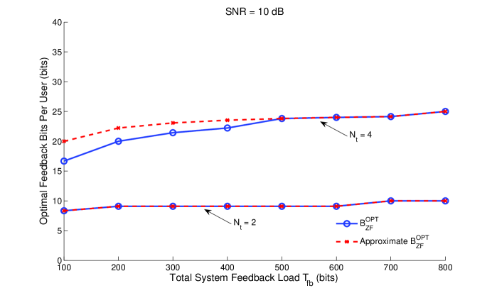
Figure 4: Behavior of $B_{\text{ZF}}^{\textsc{OPT}}\left(\mbox{\scriptsize\sf SNR},N_{t},T_{\text{fb}}\right)$ with $T_{\text{fb}}$

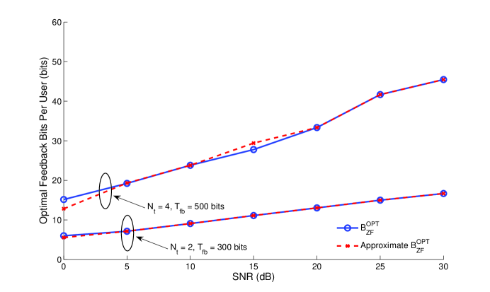
Figure 5: Behavior of $B_{\text{ZF}}^{\textsc{OPT}}\left(\mbox{\scriptsize\sf SNR},N_{t},T_{\text{fb}}\right)$ with SNR

In Figures 4 and 5, $B_{\text{ZF}}^{\textsc{OPT}}\left(\mbox{\scriptsize\sf SNR},N_{t},T_{\text{fb}}\right)$ and the approximation $\widetilde{B}_{\text{ZF}}^{\textsc{OPT}}\left(\mbox{\scriptsize\sf SNR},N_{t},T_{\text{fb}}\right)$ are plotted versus $T_{\text{fb}}$ and $\mbox{\scriptsize\sf SNR}_{\text{dB}}$, respectively. In both figures we see that the approximation is quite accurate, and that the behavior agrees with the scaling relationships in (16) and (18). Curves for $N_{t}=2$ and $N_{t}=4$ are included in both figures, and $B_{\text{ZF}}^{\textsc{OPT}}$ is seen to increase roughly with $N_{t}-1$, consistent with (17).

V Optimization of $\text{PU}^{2}\text{RC}$

As described in Section III-C, Per unitary basis stream user and rate control ($\text{PU}^{2}\text{RC}$) generalizes RBF to more than $\log_{2}N_{t}$ feedback bits per user. A common quantization codebook, consisting of $2^{B}/N_{t}$ ‘sets’ of $N_{t}$ orthoognal vectors each, is utilized by each user. A user finds the best of the $2^{B}$ quantization vectors, accordng to (2), and feeds back the index of the set ($B-\log_{2}N_{t}$ bits) and the index of the vector/beam in that set ($\log_{2}N_{t}$ bits). Although the quantization codebooks for ZF and $\text{PU}^{2}\text{RC}$ are slightly different, the key difference is in user selection. While ZF allows for selection of any subset of (up to) $N_{t}$ users, the low-complexity $\text{PU}^{2}\text{RC}$ procedure described in Section III-C constrains the BS to select a set of up to $N_{t}$ users from one of the $2^{B}/N_{t}$ sets.

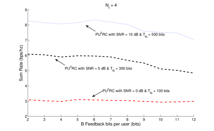
Figure 6: Sum rate vs $B$ for PU²RC with $N_{t}=4$

As a result of this difference, a very different conclusion is reached when we optimize the per-user feedback load $B$ for $\text{PU}^{2}\text{RC}$: we find that $B=\log_{2}N_{t}$ (i.e., RBF) is near-optimal and thus the optimization provides little advantage. Sum rate is plotted versus $B$ (for $\text{PU}^{2}\text{RC}$) in Figure 6. Very different from ZF, the sum rate does not increase rapidly with $B$ for small $B$, and it begins to decrease for even moderate values of $B$.

If $B$ is too large, the number of orthogonal sets $2^{B}/N_{t}$ becomes comparable to the number of users $T_{\text{fb}}/B$ and thus it is likely that there are fewer than $N_{t}$ users on every set (there are on average $\frac{T_{\text{fb}}N_{t}}{B2^{B}}$ users per set). For example, if $T_{\text{fb}}=500$ and $B=8$, there are $2^{6}$ orthogonal sets and $40$ users and thus less than a user per set on average. Hence, the BS likely schedules much fewer than $N_{t}$ users, thereby leading to a reduced sum rate. Thus, large values of $B$ are not preferred.

For moderate values of $B>\log_{2}N_{t}$, there are a sufficient number of users per set but nonetheless this ‘thinning’ of users is the limiting factor. As $B$ increases the quantization quality increases, but because there are only $\frac{T_{\text{fb}}N_{t}}{B2^{B}}$ users per set (on average) the multi-user diversity (in each set) decreases sharply, so much so that the rate per set in fact decreases with $B$. (For ZF there is also a loss in multi-user diversity as $B$ is increased, but the number of users is inversely proportional to $B$, whereas here it is inversely proportional to $B2^{B}$.) The BS does choose the best set (amongst the $2^{B}/N_{t}$ sets), but this is not enough to compensate for the decreasing per-set rate.

VI Comparison of Multi-user Beamforming Schemes

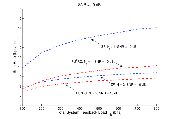
Figure 7: ZF vs. PU²RC sum rate with optimized $B$

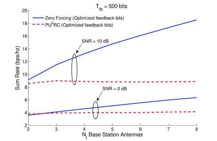
Figure 8: Sum rate vs. $N_{t}$ with optimized $B$ and $T_{\text{fb}}=500$ bits

In Figure 7, the sum rates of ZF and PU²RC are compared for various values of SNR, $T_{\text{fb}}$ and $N_{t}$; for each strategy, $B$ has been optimized separately as discussed in Sections IV and V, respectively. It is seen that ZF maintains a significant advantage over PU²RC for $N_{t}=4$. At small $N_{t}$, both schemes perform similarly, but ZF maintains a small advantage. In addition, the advantage of ZF increases extremely rapidly with $N_{t}$ and SNR. For example, Figure 8 compares the sum rate of the two strategies with varying $N_{t}$ for $T_{\text{fb}}=500$ bits. The basic conclusion is that optimized ZF significantly outperforms optimized PU²RC. This holds for essentially all system parameters ($N_{t}$, SNR, $T_{\text{fb}}$) of interest, with the only exception being $N_{t}=2$ around 0 dB.

As optimized PU²RC performs essentially the same as RBF (Section V), this large gap in sum rate can be explained by contrasting RBF and optimized ZF. In particular, it is useful to find the number of users needed by RBF to match the sum rate of optimized ZF. From [1], we have that the SINR of the $k^{\text{th}}$ user (on a particular beam) under RBF has CDF $1-\frac{e^{-x\frac{N_{t}}{\mbox{\scriptsize\sf SNR}}}}{(x+1)^{N_{t}-1}}$. With $K$ users in the system, RBF chooses the largest SINR amongst these $K$ users (this is in fact an upper bound as explained in [1]). By basic results in order statistics, the expectation of the maximum amongst $K$ i.i.d. random variables is accurately approximated by the point at which the CDF equals $(K-1)/K$ [18]. Hence, in order to achieve a target SINR $S$, RBF requires approximately $K=\exp\left(\frac{SN_{t}}{\mbox{\scriptsize\sf SNR}}\right)\left(1+S\right)^{N_{t}-1}$ users. From Section IV, optimized ZF operates with effectively perfect CSI. Hence, dropping the interference term in (8), we have that ZF achieves an SINR of about $\frac{\mbox{\scriptsize\sf SNR}}{N_{t}}\log\frac{T_{\text{ZF}}N_{t}}{B_{ZF}^{OPT}}$, for a total feedback budget of $T_{\text{ZF}}$ bits. Setting $S=\frac{\mbox{\scriptsize\sf SNR}}{N_{t}}\log\frac{T_{\text{ZF}}N_{t}}{B_{ZF}^{OPT}}$, we see that RBF requires approximately $K=\frac{T_{\text{ZF}}N_{t}}{B_{ZF}^{OPT}}\left(1+\frac{\mbox{\scriptsize\sf SNR}}{N_{t}}\log\frac{T_{\text{ZF}}N_{t}}{B_{ZF}^{OPT}}\right)^{N_{t}-1}$ users to match the SINR achieved by optimized ZF for a given $T_{\text{ZF}}$, $N_{t}$ and SNR. The total feedback for RBF is $T_{\text{RBF}}=K\log_{2}N_{t}$ bits. Thus RBF requires approximately $T_{\text{RBF}}$ total bits to match the sum rate of optimized ZF with $T_{\text{ZF}}$ bits, where

$$T_{\text{RBF}} = \left(\log_{2}N_{t}\right)\frac{T_{\text{ZF}}N_{t}}{B_{ZF}^{OPT}}\left(1+\frac{\mbox{\scriptsize\sf SNR}}{N_{t}}\log\frac{T_{\text{ZF}}N_{t}}{B_{ZF}^{OPT}}\right)^{N_{t}-1}.$$ (19)

For example, when $N_{t}=4$, $\mbox{\scriptsize\sf SNR}=5$ dB and $T_{\text{fb}}=300$ bits, RBF requires $5000$ users, and thus 10000 bits, in order to match the sum rate of ZF with only $300$ bits. Clearly, it is impractical to consider RBF in such a setting. Furthermore, from (19) we have that $T_{\text{RBF}}$ increases rapidly with $T_{\text{ZF}}$, $N_{t}$ as well as SNR, making RBF increasingly impractical.

Although RBF uses a very small codebook of $N_{t}$ vectors, it may appear that this is compensated by the large number of users $T_{\text{fb}}/\log_{2}N_{t}$. By selecting users with large SINR’s, the BS exploits multi-user diversity and selects users that have channels with large norms and that are well-aligned to one of the $N_{t}$ quantization vectors/beamformers. The latter of these two effects can be referred to as ‘quantization diversity’, and it may seem that this effect can compensate for the very small codebook. However, it turns out to be very unlikely that a selected user is well-aligned with its quantization vector, even if $T_{\text{fb}}$ is very large. To see this, consider the smallest quantization error amongst the $T_{\text{fb}}/\log_{2}N_{t}$ users. Because the user channels are independent and spatially isotropic, the smallest error is precisely the same, in distribution, as the quantization error for a single user quantizing to a codebook of $T_{\text{fb}}/\log_{2}N_{t}$ orthogonal sets of $N_{t}$ vectors each, where each orthogonal set is independent and isotropic. Thus, the smallest quantization error for RBF is effectively the same as that of a codebook of size $B=\log_{2}\left(T_{\text{fb}}N_{t}/\log_{2}N_{t}\right)$. For example, with $N_{t}=4$ and $T_{\text{fb}}=300$ bits, the best quantization error is only as good as an 8-bit quantization. As we saw in Section IV, the sum rate is very sensitive to quantization error and multi-user diversity cannot compensate for this.

VII Further Considerations

VII-A Effect of Optimal User Selection and SINR Feedback

In this section, we will argue that the choice of CQI (for ZF) does not significantly alter our main results, and that it is not necessary to use high-complexity user selection algorithms to benefit from the optimization of $B$.

In terms of CQI for ZF, we have thus far considered channel norm feed back. An alternative is feeding back the expected SINR (as discussed in [17])

$$\frac{||{\bf h}_{k}||^{2}\cos^{2}\left(\angle({\bf h}_{k},\widehat{{\bf h}}_{k})\right)}{\frac{N_{t}}{\mbox{\scriptsize\sf SNR}}+||{\bf h}_{k}||^{2}\sin^{2}\left(\angle({\bf h}_{k},\widehat{{\bf h}}_{k})\right)}$$ (20)

as is done for RBF/PU²RC. This allows the BS to select users that have not only large channels, but also small quantization errors. In [17, Eq. (41)], the rate achievable with SINR feedback when the number of users feeding back is large increases with the quantity $2^{B}\frac{T_{\text{fb}}}{B}$, and this increases monotonically in $B$ (for $B>2$). Thus, the sum rate (with SINR feedback) increases with $B$ as long as one remains in the large user regime, as described in [17], eventually entering the high resolution regime (provided $T_{\text{fb}}$ is sufficiently large). However, in this regime, the advantage of SINR feedback over channel norm feedback is minimal as the quantization error is small, and there is no real difference between the two CQI feedback schemes. On the other hand, if $T_{\text{fb}}$ is very small so that one cannot really enter the high resolution regime, SINR-based feedback is seen to provide a slightly larger sum rate than norm feedback, but the optimal value of $B$ is largely the same.

The primary disadvantage of the ZF technique we have considered so far is the relatively high complexity user selection algorithm. We now illustrate that ZF is superior to RBF/PU²RC even when a much lower complexity selection algorithm is used. In particular, we consider the following algorithm: the BS sorts the $T_{\text{fb}}/B$ users by channel norm, computes the ZF rate for the users with the $j$ largest channel norms for $j=1,\ldots,N_{t}$, and then picks the $j$ that provides the largest sum rate. This requires $N_{t}$ sum rate computations, whereas the greedy selection algorithm of [10] performs an order of $N_{t}(T_{\text{fb}}/B)$ rate computations. The selected user set is likely to have fewer and less orthogonal users than greedy selection and thus performs significantly worse than greedy selection, but nonetheless is seen to outperform PU²RC.

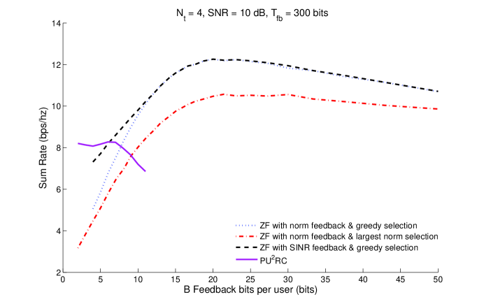
Figure 9: Sum rate with optimized $B$ and various user selection schemes with $N_{t}=4,T_{\text{fb}}=300$ bits and $\mbox{\scriptsize\sf SNR}=10$ dB

In Figure 9 sum rate is plotted versus $B$ for norm and SINR feedback (for greedy selection), and for greedy and simplified user selection (for norm feedback). In terms of CQI feedback, for small $B$ the sum rate with SINR feedback is slightly larger than with norm-feedback but this advantage vanishes for large $B$, which is the optimal operating point. In terms of user selection, we see that the simplified approach achieves a much smaller sum rate than the greedy algorithm but still outperforms PU²RC. Although this simplified scheme may not be the best low-complexity search algorithm, this simply illustrates that user selection complexity need not be a major concern with respect to our main conclusion.

VII-B Effect of Receiver Training and Feedback Delay

If there is imperfect CSI at the users and/or delay in the channel feedback loop, then there is some inherent imperfection in the CSI provided to the BS, even if $B$ is extremely large. As we will see, this only corresponds to a shift in the system SNR and thus does not affect our basic conclusions.

We model the case of receiver training as described in [19]. To permit each user to estimate its own channel, $\beta N_{t}$ (shared) downlink pilots (or $\beta$ pilots per antenna) are transmitted. If each user performs MMSE estimation, the estimate $\tilde{{\bf h}}_{k}$ (of ${\bf h}_{k}$) and ${\bf h}_{k}$ are related as ${\bf h}_{k}=\tilde{{\bf h}}_{k}+{\bf n}_{k}$, where ${\bf n}_{k}$ is the Gaussian estimation error of variance $(1+\beta\ \mbox{\scriptsize\sf SNR})^{-1}$. To model feedback delay we consider correlated block fading where ${\bf h}_{k}$ is the channel during receiver training and feedback while ${\bf h}_{k}^{+}$ is the channel during actual data transmission, with the two related according to ${\bf h}_{k}^{+}=r\ {\bf h}_{k}+\sqrt{1-r^{2}}\ \Delta_{k}$, where $0<r<1$ is the correlation coefficient and $\Delta_{k}$ is a standard complex Gaussian process. User $k$ quantizes its channel estimate $\widetilde{{\bf h}}_{k}$ and feeds this back to the BS. Following the same methods used for (8) and the argument in [19], the combined effect of the estimation error at the user and the feedback delay changes our sum rate approximation to:

$$\widetilde{R}_{\textsc{Training-Delay}}\left(\mbox{\scriptsize\sf SNR},N_{t},\frac{T_{\text{fb}}}{B},B\right) = N_{t}\ \log_{2}\left[1+\frac{\frac{\mbox{\scriptsize\sf SNR}}{N_{t}}\log\frac{T_{\text{fb}}N_{t}}{B}}{1+\phi\frac{N_{t}}{N_{t}-1}\mbox{\scriptsize\sf SNR}+\frac{\mbox{\scriptsize\sf SNR}}{N_{t}}2^{-\frac{B}{N_{t}-1}}\log\frac{T_{\text{fb}}N_{t}}{B}}\right],$$ (21)

where the term $\phi=1-r^{2}+(1+\beta\ \mbox{\scriptsize\sf SNR})^{-1}$ is the additional multi-user interference due to training and delay. This approximation is the same as $\widetilde{R}_{\textsc{ZF}}\left(\frac{\mbox{\scriptsize\sf SNR}}{1+\phi\frac{N_{t}}{N_{t}-1}\mbox{\scriptsize\sf SNR}},N_{t},\frac{T_{\text{fb}}}{B},B\right)$, and thus we see that training and delay simply reduce the system SNR. Hence, all previously discussed results continue to apply, although with a shift in system SNR.

VII-C Low-complexity Quantization

Although the computational complexity of performing high-rate quantization may seem daunting, here we show that the very low-complexity scalar quantization scheme proposed in [20] provides a sum rate only slightly smaller than RVQ. In the scheme of [20], the components of channel vector ${\bf h}_{k}=\left[h_{1},\dots,h_{N_{t}}\right]^{T}$ are first divided by the first component $h_{1}$ to yield $N_{t}-1$ complex elements. The $N_{t}-1$ relative phases are individually quantized using uniform (scalar) quantization in the interval $[-\pi,\pi]$. Similarly, the inverse tangents of the relative magnitudes, i.e., $\tan^{-1}\left(\frac{|h_{m}|}{|h_{1}|}\right)$ for $m=2,\dots,N_{t}$, are each quantized uniformly in the interval $[0,\frac{\pi}{2}]$. The $B$ bits are distributed equally between the phases and magnitudes of the $N_{t}-1$ elements as far as possible.

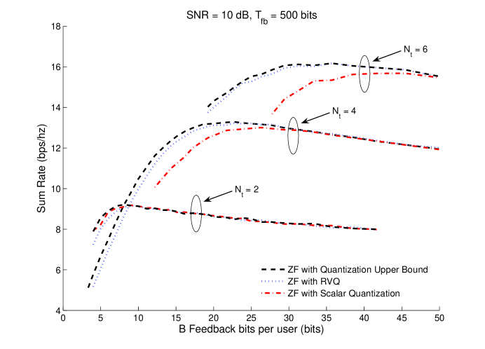
Figure 10: ZF sum rate with optimized $B$ and various quantization schemes

In Figure 10 sum rate is plotted versus $B$ for RVQ and scalar quantization at $\mbox{\scriptsize\sf SNR}=10$ dB. Scalar quantization provides a smaller sum rate than RVQ for small and moderate values of $B$, and the optimum value of $B$ for scalar quantization is a few bits larger than with RVQ. Most importantly, the optimized rate with scalar quantization is only slightly smaller than the optimized rate with RVQ (this is also true for other values of $N_{t}$, $T_{\text{fb}}$, and SNR).

The strong performance of scalar quantization can be explained through the expected angular distortion. For RVQ the expected angular distortion satisfies $\mbox{\bb E}\left[\sin^{2}\angle({\bf h}_{k},\widehat{{\bf h}}_{k})\right]\leq 2^{-\frac{B}{N_{t}-1}}$, and this term appears in the approximation in (8). By basic results on high-rate quantization, the distortion with scalar quantization is also proportional to $2^{-\frac{B}{N_{t}-1}}$ but with a larger constant [21]. This constant term translates to a constant bit penalty; for $N_{t}=4$ a numerical comparison shows a bit penalty of approximately $4.5$ bits, i.e., scalar quantization with $B+4.5$ bits achieves the same distortion as RVQ with $B$ bits. As a result, scalar quantization requires a large value of $B$ in order to achieve near-perfect CSI, but because CSI is strongly preferred to multi-user diversity it is still worthwhile to operate at the ”essentially perfect” CSI point, even with a suboptimal quantization codebook.

In order to show that it is not possible to greatly improve upon RVQ, in Figure 10 the sum rate with an idealized codebook that achieves the quantization upper bound given in [22] is also shown. The expected distortion of this idealized codebook is only a factor of $\frac{N_{t}-1}{N_{t}}$ smaller than with RVQ, and thus a very small performance gap is expected.

VII-D Effect of CQI Quantization

Prior work has shown that CQI quantized to 3-4 bits (per user) is virtually the same as unquantized CQI [9][17]. Since the actual per-user feedback is the $B$ directional bits plus the CQI bits, by ignoring CQI bits in the feedback budget we have artificially inflated the number of users. If the CQI bits are accounted for, strategies that utilize few directional bits become even less attractive (CQI bits make multi-user diversity more expensive) and thus our basic conclusion is unaffected. For example, with $N_{t}=4$, $T_{\text{fb}}=300$ bits and $\mbox{\scriptsize\sf SNR}=10$ dB, ZF with unquantized CQI (i.e., not accounting for CQI feedback) is optimized with 13 users and $B=23$. If, on the other hand, we actually quantize the CQI to $4$ bits and then allow only $\frac{T_{\text{fb}}}{B+4}$ users to feedback, the optimum point changes to 10 users with $B=26$.

VII-E Single-User Beamforming

In this section, we consider the case when the BS is constrained to beamform to only a single user. Each user quantizes its channel direction using $B$ bits and feeds back its quantization index, or equivalently $\widehat{{\bf h}}_{k}$, along with the received signal-to-noise ratio for beamforming along the direction $\widehat{{\bf h}}_{k}$: $\mbox{\scriptsize\sf SNR}\ |{\bf h}_{k}^{\sf H}\widehat{{\bf h}}_{k}|^{2}=\mbox{\scriptsize\sf SNR}\ ||{\bf h}_{k}||^{2}\cos^{2}\angle({\bf h}_{k},\widehat{{\bf h}}_{k})$. The BS then selects the user $k^{*}$ with the largest such post-beamforming SNR:

$$k^{*}=\mathop{\mathop{\rm argmax}}\limits_{1\leq k\leq\frac{T_{\text{fb}}}{B}}\ \mbox{\scriptsize\sf SNR}\ ||{\bf h}_{k}||^{2}\cos^{2}\left(\angle({\bf h}_{k},\widehat{{\bf h}}_{k})\right).$$ (22)

Let $R_{\textsc{SUBF}}\left(\mbox{\scriptsize\sf SNR},N_{t},\frac{T_{\text{fb}}}{B},B\right)$ be the average rate achieved with signal-to-noise ratio SNR, $N_{t}$ antennas at the BS and $T_{\text{fb}}/B$ users feeding back $B$ bits each:

$$R_{\textsc{SUBF}}\left(\mbox{\scriptsize\sf SNR},N_{t},\frac{T_{\text{fb}}}{B},B\right) = \mbox{\bb E}\left[\log_{2}\left(1+\mbox{\scriptsize\sf SNR}\ \max\limits_{1\leq k\leq\frac{T_{\text{fb}}}{B}}\ \left(||{\bf h}_{k}||^{2}\cos^{2}\left(\angle({\bf h}_{k},\widehat{{\bf h}}_{k})\right)\right)\right)\right].$$ (23)

The optimizing $B$, given $\mbox{\scriptsize\sf SNR},N_{t}$, and $T_{\text{fb}}$, is defined as:

$$B_{\text{SUBF}}^{\textsc{OPT}}\left(\mbox{\scriptsize\sf SNR},N_{t},\frac{T_{\text{fb}}}{B}\right) = \mathop{\rm argmax}_{1\leq B\leq T_{\text{fb}}}\ R_{\textsc{SUBF}}\left(\mbox{\scriptsize\sf SNR},N_{t},\frac{T_{\text{fb}}}{B},B\right)$$ (24)

However, this optimization cannot be performed analytically, so we instead find a reasonable approximation $\widetilde{R}_{\textsc{SUBF}}\left(\mbox{\scriptsize\sf SNR},N_{t},\frac{T_{\text{fb}}}{B},B\right)$ for $R_{\textsc{SUBF}}\left(\mbox{\scriptsize\sf SNR},N_{t},\frac{T_{\text{fb}}}{B},B\right)$ that is tractable.

$$R_{\textsc{SUBF}}\left(\mbox{\scriptsize\sf SNR},N_{t},\frac{T_{\text{fb}}}{B},B\right) \approx \log_{2}\left(1+\mbox{\scriptsize\sf SNR}\ \left(1+\left(1-2^{-\frac{B}{N_{t}-1}}\right)\log\frac{T_{\text{fb}}N_{t}}{B}\right)\right)$$ (25)

$$\approx \log_{2}\left[1+\mbox{\scriptsize\sf SNR}\ \left(\log\frac{T_{\text{fb}}N_{t}}{B}-2^{-\frac{B}{N_{t}-1}}\log\left(T_{\text{fb}}N_{t}\right)\right)\right]$$

$$= \widetilde{R}_{\textsc{SUBF}}\left(\mbox{\scriptsize\sf SNR},N_{t},\frac{T_{\text{fb}}}{B},B\right)$$

Equation 25 is derived in Appendix B, and (VII-E) is obtained by neglecting the term $2^{-\frac{B}{N_{t}-1}}\log B$, which is small relative to $2^{-\frac{B}{N_{t}-1}}\log\left(T_{\text{fb}}N_{t}\right)$. The corresponding approximation $\widetilde{B}_{\text{SUBF}}^{\textsc{OPT}}\left(\mbox{\scriptsize\sf SNR},N_{t},\frac{T_{\text{fb}}}{B}\right)$ for $B_{\text{SUBF}}^{\textsc{OPT}}\left(\mbox{\scriptsize\sf SNR},N_{t},\frac{T_{\text{fb}}}{B}\right)$ is:

$$\widetilde{B}_{\text{SUBF}}^{\textsc{OPT}}\left(\mbox{\scriptsize\sf SNR},N_{t},\frac{T_{\text{fb}}}{B}\right)=\mathop{\rm argmax}_{1\leq B\leq T_{\text{fb}}}\ \widetilde{R}_{\textsc{SUBF}}\left(\mbox{\scriptsize\sf SNR},N_{t},\frac{T_{\text{fb}}}{B},B\right).$$ (27)

Note that $\widetilde{B}_{\text{SUBF}}^{\textsc{OPT}}\left(\mbox{\scriptsize\sf SNR},N_{t},\frac{T_{\text{fb}}}{B}\right)$ is independent of SNR. Maximizing the concave function (VII-E) with respect to $B$ yields the following solution:

$$\widetilde{B}_{\text{SUBF}}^{\textsc{OPT}}\left(\mbox{\scriptsize\sf SNR},N_{t},\frac{T_{\text{fb}}}{B}\right) = -\frac{(N_{t}-1)}{\log 2}\ W_{-1}\left(-\frac{1}{\log\left(T_{\text{fb}}N_{t}\right)}\right)$$ (28)

$$\sim (N_{t}-1)\log_{2}\log\left(T_{\text{fb}}N_{t}\right)+O(\log\log(N_{t}\log T_{\text{fb}}))$$ (29)

where $W_{-1}(\cdot)$ is branch -1 of the LambertW function and (29) is obtained through asymptotic expansion [16]. $\widetilde{B}_{\text{SUBF}}^{\textsc{OPT}}\left(\mbox{\scriptsize\sf SNR},N_{t},\frac{T_{\text{fb}}}{B}\right)$ is truncated to be between $1$ and $T_{\text{fb}}$. Note that the optimal number of bits scale roughly linearly with $N_{t}$, provided $T_{\text{fb}}$ is sufficiently large, and double logarithmically with $T_{\text{fb}}$.

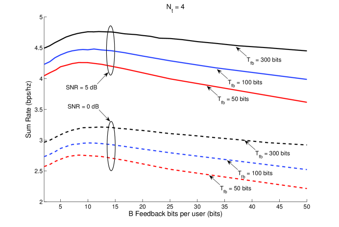
Figure 11: Sum rate vs. Feedback load for Single-user Beamforming with $N_{t}=4$

Figure 11 depicts the behavior of rate with $B$ for a $4$ antenna system at $0$ and $5$ dB. Although there clearly is a peak for all of the curves, very different from multi-user beamforming, the sum rate is not particularly sensitive to $B$ and thus using the optimizing $B$ provides only a small rate advantage. Multi-user beamforming systems are extremely sensitive to CSI because the interference power depends critically on the CSI; for single-user beamforming there is no interference and thus the dependence upon CSI is much weaker.

VIII Conclusion

In this paper, we have considered the basic but apparently overlooked question of whether low-rate feedback/many user systems or high-rate feedback/limited user systems provide a larger sum rate in MIMO downlink channels. This question simplifies to a comparison between multi-user diversity (many users) and accurate channel information (high-rate feedback), and the surprising conclusion is that there is a very strong preference for accurate CSI. Multi-user diversity provides a throughput gain that is only double-logarithmic in the number of users who feed back, whereas the marginal benefit of increased per-user feedback is very large up to the point where the CSI is essentially perfect.

Although we have considered only spatially uncorrelated Rayleigh fading with independent fading across blocks, our general conclusion applies to more realistic fading models. A channel with strong spatial correlation is easier to describe (assuming appropriate quantization) than an uncorrelated channel and thus fewer bits are required to achieve essentially perfect CSI. For example, $15$/$20$ bits might be required to provide nearly perfect CSI for a $4$-antenna channel at $10$ dB with/without correlation, respectively. Thus, spatial correlation further reinforces the preference towards accurate CSI. In terms of channel correlation across time and frequency, we note that a recent work has studied a closely related tradeoff in the context of a frequency-selective channel [23]: should each user quantize its entire frequency response or only a small portion of the frequency response (i.e., quantize only a single resource block)? The first option corresponds to coarse CSI (even though frequency-domain correlation is exploited) but a large user population, while the second corresponds to accurate CSI but fewer users per resource block. Consistent with our results, the second option is seen to provide a considerably larger sum rate than the first. We suspect the same holds true in the context of temporal correlation, where the comparison is between a user quantizing its channel across many continuous blocks (possibly exploiting the correlation of the channel by using a differential quantization scheme) and a user finely quantizing its current channel at only a few limited time instants.

In closing, it is worth emphasizing that our results do not imply that multi-user diversity is worthless. On the contrary, multi-user diversity does provide a significant benefit. However, the basic design insight is that feedback resources should first be used to obtain accurate CSI and only afterwards be used to exploit multi-user diversity. Given the increasing importance of multi-user MIMO in single-cell and multi-cell (i.e., network MIMO) settings, it seems that this point should be fully exploited in the design of next-generation cellular systems such as LTE.

Appendix A Order Statistics of a $\Gamma(N_{t},1)$ random variable

Let $X^{(K)}_{1:K}$ be the $K^{\text{th}}$ order statistic among $X_{1},X_{2},\dots,X_{K}$ which are $K$ i.i.d. $\Gamma(N_{t},1)$ random variables. Note that $X_{k}$ has the same distribution of $Y_{k,1}+Y_{k,2}+\dots+Y_{k,N_{t}}$, where $Y_{k,1},Y_{k,2},\dots,Y_{k,N_{t}}$ are i.i.d. $\Gamma(1,1)$ variates. $\mbox{\bb E}\left[X^{(K)}_{1:K}\right]$ is not known in closed form, and we will hence use the following lower bound:

$$\mbox{\bb E}\left[X^{(K)}_{1:K}\right] = \max\limits_{k=1,\dots,K}\ Y_{k,1}+Y_{k,2}+\dots+Y_{k,N_{t}}$$ (30)

$$\geq \max\limits_{k=1,\dots,K}\ \max\limits_{n=1,\dots,N_{t}}\ Y_{k,n}$$ (31)

$$= \sum\limits_{k=1}^{KN_{t}}\frac{1}{k}$$ (32)

$$\sim \log(KN_{t})+\gamma,$$ (33)

where (32) is obtained from [18, 2.7.5] and (33) holds as $K\rightarrow\infty$ where $\gamma$ is the Euler-Mascheroni constant. Equation 33 implies a logarithmic growth in $K$, as described in, for example, [24]. We will typically apply (33) while omitting the Euler-Mascheroni constant for simplicity.

Appendix B Approximation for $R_{\textsc{SUBF}}\left(\mbox{\scriptsize\sf SNR},N_{t},\frac{T_{\text{fb}}}{B},B\right)$

Recall from (23), that:

$$R_{\textsc{SUBF}}\left(\mbox{\scriptsize\sf SNR},N_{t},\frac{T_{\text{fb}}}{B},B\right) = \mbox{\bb E}\left[\log_{2}\left(1+\mbox{\scriptsize\sf SNR}\max\limits_{1\leq k\leq\frac{T_{\text{fb}}}{B}}\left(||{\bf h}_{k}||^{2}\cos^{2}\left(\angle({\bf h}_{k},\widehat{{\bf h}}_{k})\right)\right)\right)\right]$$ (34)

$$\leq \log_{2}\left(1+\mbox{\scriptsize\sf SNR}\ \mbox{\bb E}\left[\max\limits_{1\leq k\leq\frac{T_{\text{fb}}}{B}}\left(||{\bf h}_{k}||^{2}\cos^{2}\left(\angle({\bf h}_{k},\widehat{{\bf h}}_{k})\right)\right)\right]\right)$$ (35)

$$= \log_{2}\left(1+\mbox{\scriptsize\sf SNR}\ \mbox{\bb E}\left[\max\limits_{1\leq k\leq\frac{T_{\text{fb}}}{B}}\left(G_{k}^{(1)}+\left(1-2^{-\frac{B}{N_{t}-1}}\right)\ G_{k}^{(N_{t}-1)}\right)\right]\right)$$ (36)

$$\approx \log_{2}\left(1+\mbox{\scriptsize\sf SNR}\ \mbox{\bb E}\left[\left(G_{k}^{(1)}+\left(1-2^{-\frac{B}{N_{t}-1}}\right)\ \max\limits_{1\leq k\leq\frac{T_{\text{fb}}}{B}}G_{k}^{(N_{t}-1)}\right)\right]\right)$$

$$= \log_{2}\left(1+\mbox{\scriptsize\sf SNR}\left(\mbox{\bb E}\left[G_{k}^{(1)}\right]+\left(1-2^{-\frac{B}{N_{t}-1}}\right)\ \mbox{\bb E}\left[\max\limits_{1\leq k\leq\frac{T_{\text{fb}}}{B}}G_{k}^{(N_{t}-1)}\right]\right)\right)$$

$$= \log_{2}\left(1+\mbox{\scriptsize\sf SNR}\left(1+\left(1-2^{-\frac{B}{N_{t}-1}}\right)\mbox{\bb E}\left[\max\limits_{1\leq k\leq\frac{T_{\text{fb}}}{B}}G_{k}^{(N_{t}-1)}\right]\right)\right)$$ (38)

$$\approx \log_{2}\left(1+\mbox{\scriptsize\sf SNR}\left(1+\left(1-2^{-\frac{B}{N_{t}-1}}\right)\left(\log\frac{T_{\text{fb}}N_{t}}{B}\right)\right)\right)$$ (39)

where (35) is obtained by applying Jensen’s inequality. Equation 36 is obtained from [17, Lemma 2], where $G^{(m)}_{k}$ in (36) is a $\Gamma(m,1)$ variate. Equation B is obtained by restricting the maximization to apply only to the $G^{(N_{t}-1)}_{k}$ (which stochastically dominates $G^{(1)}_{k}$), and the expectation in (38) has been replaced by (33) from Appendix A after neglecting the Euler-Mascheroni constant.

Figure 1: Feedback of channel information in a MIMO downlink system

References

- [1] M. Sharif and B. Hassibi, “On the capacity of MIMO broadcast channels with partial side information,” IEEE Tran. on Inform. Theory, vol. 51, no. 2, pp. 506–522, 2005.
- [2] http://www.ece.umn.edu/users/nihar/mud_csi_code.html.
- [3] R. Zakhour and D. Gesbert, “A two-stage approach to feedback design in MU-MIMO channels with limited channel state information,” in Proc. IEEE Personal, Indoor and Mobile Radio Commun. Symp., 2008, pp. 111–115.
- [4] K. Huang, J. Andrews, and R. Heath, “Performance of Orthogonal Beamforming for SDMA with Limited Feedback,” IEEE Tran. Vehicular Tech., 2007.
- [5] C. Swannack, G. Wornell, and E. Uysal-Biyikoglu, “MIMO Broadcast Scheduling with Quantized Channel State Information,” in Proc. IEEE Int. Symp. on Inform. Theory, 2006, pp. 1788–1792.
- [6] R. Agarwal, C. Hwang, and J. Cioffi, “Scalable feedback protocol for achieving sum-capacity of the MIMO BC with finite feedback,” Stanford Technical Report, 2006.
- [7] A. Bayesteh and A. Khandani, “On the user selection for MIMO broadcast channels,” in Proc. IEEE Int. Symp. on Inform. Theory, 2005, pp. 2325–2329.
- [8] D. Gesbert and M. Alouini, “How much feedback is multi-user diversity really worth?” in Proc. IEEE Int. Conf. on Commun., vol. 1, 2004.
- [9] K. Huang, R. Heath, and J. Andrews, “Space division multiple access with a sum feedback rate constraint,” IEEE Tran. on Sig. Proc., vol. 55, no. 7 Part 2, pp. 3879–3891, 2007.
- [10] G. Dimic and N. Sidiropoulos, “On downlink beamforming with greedy user selection: performance analysis and a simple new algorithm,” IEEE Tran. on Sig. Proc., vol. 53, no. 10 Part 1, pp. 3857–3868, 2005.
- [11] W. Santipach and M. Honig, “Asymptotic capacity of beamforming with limited feedback,” in Proc. IEEE Int. Symp. on Inform. Theory, 2004.
- [12] N. Jindal, “Antenna combining for the MIMO downlink channel,” IEEE Transactions on Wireless Communications, vol. 7, no. 10, pp. 3834–3844, 2008.
- [13] ——, “MIMO Broadcast Channels with Finite Rate Feedback,” IEEE Tran. on Inform. Theory, 2006.
- [14] P. Viswanath, D. Tse, and R. Laroia, “Opportunistic beamforming using dumb antennas,” IEEE Tran. on Inform. Theory, vol. 48, no. 6, pp. 1277–1294, 2002.
- [15] J. Kim, H. Kim, C. Park, and K. Lee, “On the performance of multiuser MIMO systems in WCDMA/HSDPA: Beamforming, feedback and user diversity,” IEICE Trans. on Commun., vol. 89, no. 8, pp. 2161–2169, 2006.
- [16] R. Corless, G. Gonnet, D. Hare, D. Jeffrey, and D. Knuth, “On the LambertW function,” Advances in Computational mathematics, vol. 5, no. 1, pp. 329–359, 1996.
- [17] T. Yoo, N. Jindal, and A. Goldsmith, “Multi-antenna downlink channels with limited feedback and user selection,” IEEE J. on Select. Areas in Commun., vol. 25, no. 7, pp. 1478–1491, 2007.
- [18] H. David and H. Nagaraja, Order statistics. Wiley-Interscience, 2004.
- [19] G. Caire, N. Jindal, M. Kobayashi, and N. Ravindran, “Multiuser MIMO achievable rates with downlink training and channel state feedback,” Submitted to: IEEE Trans. Inform. Theory, 2007.
- [20] A. Narula, M. J. Lopez, M. D. Trott, G. W. Wornell, M. Inc, and M. A. Mansfield, “Efficient use of side information in multiple-antenna data transmission over fading channels,” IEEE J. on Select. Areas in Commun., vol. 16, no. 8, pp. 1423–1436, 1998.
- [21] A. Gersho and R. Gray, Vector quantization and signal compression. Springer, 1992.
- [22] S. Zhou, Z. Wang, and G. Giannakis, “Performance Analysis for Transmit-Beamforming with Finite-Rate Feedback.”
- [23] M. Trivellato, S. Tomasin, and N. Benvenuto, “On Channel Quantization and Feedback Strategies for Multiuser MIMO-OFDM Downlink Systems,” To appear: IEEE Tran. Commun., 2008.
- [24] T. Yoo and A. Goldsmith, “On the optimality of multiantenna broadcast scheduling using zero-forcing beamforming,” IEEE J. on Select. Areas in Commun., vol. 24, no. 3, pp. 528–541, 2006.