Multiwavelength Observations of Mrk 501 in 2008

Abstract

The well-studied VHE ($E>100\ \mathrm{GeV}$) blazar Mrk 501 was observed between March and May 2008 as part of an extensive multiwavelength observation campaign including radio, optical, X-ray and VHE gamma-ray instruments. Mrk 501 was in a low state of activity during the campaign, with a low VHE flux of about 20% the Crab Nebula flux. Nevertheless, significant flux variations could be observed in X-rays as well as $\gamma$-rays. Overall Mrk 501 showed increased variability when going from radio to $\gamma$-ray energies.
The broadband spectral energy distribution during the two different emission states of the campaign was well described by a homogeneous one-zone synchrotron self-Compton model. The high emission state was satisfactorily modeled by increasing the amount of high energy electrons with respect to the low emission state. This parameterization is consistent with the energy-dependent variability trend observed during the campaign.

Blazar, Mrk 501, SSC model

1 Introduction

Mrk 501 is a well-studied nearby (redshift $z=0.034$) blazar which was first detected at TeV energies by the Whipple collaboration in 1996 [1]. In subsequent years Mrk 501 was regularly observed and detected in VHE $\gamma$-rays by many other Cherenkov telescope experiments. In particular during the whole year 1997 when it showed an exceptionally strong outburst with peak flux levels up to 10 times the Crab Nebula flux and flux-doubling time scales down to 0.5 days [2]. Mrk 501 also showed strong flaring activity at X-ray energies during that year. The X-ray spectrum obtained was very hard and the synchrotron peak was found to be at $\sim 100\ \mathrm{keV}$, about 2 orders of magnitude higher than in previous observations [3]. In the following years, Mrk 501 showed only low $\gamma$-ray emission (of the order of 20-30% the Crab Nebula flux), apart from a few single flares of higher intensity. In 2005, the MAGIC telescope was able to observe Mrk 501 during another high-emission state which, although at a lower flux level compared to 1997, showed flux variations of an order of magnitude and unprecedented flux doubling time scales (down to a few minutes) [4]. Mrk 501 has been the target of many multiwavelength (MWL) campaigns (e.g. [5, 6, 7, 8]), mainly covering the object during flaring activity.
The data presented here were taken between March 25th and May 16th, 2008 during an extended MWL campaign covering radio (Effelsberg, IRAM, Medicina, Metsähovi, Noto, RATAN-600, VLBA), optical (KVA), UV (Swift/UVOT), X-ray (RXTE/PCA, Swift/XRT and Swift/BAT) and $\gamma$-ray (MAGIC, Whipple, VERITAS) energies. The duration as well as the energy coverage of this particular Mrk 501 campaign are rather unique. Details on the participating instruments and the data analysis will be presented in an upcoming paper [9].

2 Light Curves

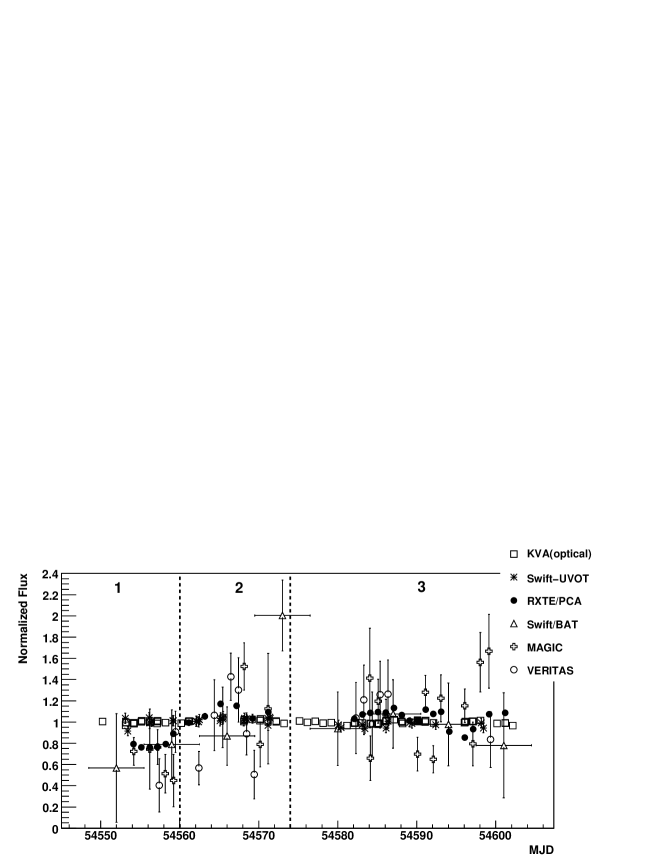
Figure 1: Combined normalized light curves for a selection of the instruments taking part in the campaign. The vertical bars denote $1\ \sigma$ statistical uncertainties, and the horizontal bars the integration time of the observation.

Figure 1 shows the normalized light curves for a selection of the instruments involved in the campaign. The different light curves cover the optical $R$ band (KVA), the UV band (Swift/UVOT), the soft X-ray band (RXTE/PCA), the hard X-ray band (Swift/BAT) and the VHE band (MAGIC and VERITAS). The average fluxes for each instrument are given as: $4.4\ \mathrm{mJy}$ (KVA), $1.6\ \mathrm{mJy}$ (Swift/UVOT), $2.8\cdot 10^{-4}\mathrm{counts/s}$ (Swift/BAT), $8.2\cdot 10^{-11}\mathrm{erg/cm^{2}/s}$ (RXTE/PCA), $2.7\cdot 10^{-11}\mathrm{ph/cm^{2}/s}$ (MAGIC) and $2.2\cdot 10^{-11}\mathrm{ph/cm^{2}/s}$ (VERITAS). Other instruments providing valuable data (like Swift/XRT or Whipple) have been omitted for the sake of clarity in this plot. Flux variations are large in X-rays and $\gamma$-rays, but rather small in the UV and optical. Due to the small error bars in the X-ray data, the most significant flux variations can be observed at these energies. The plot also shows some evidence for a correlated flux variability at X-rays and VHE $\gamma$-rays (see section 4) indicating a low-emission state before MJD 54560 and a somewhat stronger emission afterwards. For the spectral analysis presented below we divided the data set into three time intervals taking into account the X-ray flux level (i.e. low/high flux before/after MJD 54560) and the data gap at most frequencies around MJD 54574.

3 Variability

We followed the description given in [10] to quantify the flux variability by means of the so-called fractional variability parameter $F_{\mathrm{var}}$. In order to account for the individual flux measurement errors ($\sigma_{\mathrm{err,i}}$), the ‘excess variance’ ([11, 12]) was used as an estimator of the intrinsic source flux variance. This is the variance after subtracting the contribution expected from measurement errors. $F_{\mathrm{var}}$ was derived for each individual instrument taking part in the campaign, which covered an energy range from radio frequencies at $\sim$8 GHz up to very high energies at $\sim$10 TeV. $F_{\mathrm{var}}$ is calculated as:

$$F_{\mathrm{var}}=\sqrt{\frac{S^{2}-<\sigma_{\mathrm{err}}^{2}>}{<F_{\gamma}>^{2}}}$$ (1)

where $<F_{\gamma}>$ denotes the average photon flux, $S$ the standard deviation of the $N$ flux measurements and $<\sigma_{\mathrm{err}}^{2}>$ the mean squared error, all determined for a given instrument (energy bin). The uncertainty of $F_{\mathrm{var}}$ is estimated according to:

$$\Delta F_{\mathrm{var}}=\frac{<\sigma_{\mathrm{err}}^{2}>}{\sqrt{N}<F_{\gamma}>}\cdot\sqrt{1+\frac{1}{2<F_{\gamma}>^{2}F_{\mathrm{var}}^{2}}}$$

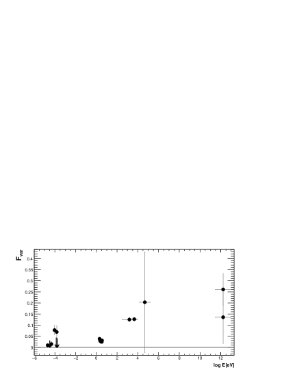
Figure 2: Fractional variability parameter $F_{\mathrm{var}}$ for all the instruments participating in the campaign. $F_{\mathrm{var}}$ was derived using the individual single-night flux measurements except for Swift/BAT for which data integrated over one week were used. Vertical bars denote $1\ \sigma$ uncertainties, horizontal bars indicate the approximate energy range covered by the instrument. The arrows indicate 95% confidence level upper limits.

Fig. 2 shows the $F_{\mathrm{var}}$ values derived for all instruments that participated in the MWL campaign. Some instruments showed a negative excess variance ($<\sigma_{\mathrm{err}}^{2}>$ larger than $S^{2}$), which can happen when there is little variability and/or the errors are slightly overestimated. Essentially such a result can be interpreted as no signature for variability in the data of that particular instrument, either because a) there was no variability or b) the instrument was not sensitive enough to detect it. In these cases, upper limits of 95% confidence level were computed.
The plot, on the other hand, also shows significant variability detected with various other instruments during the campaign. Essentially all instruments observing at optical or larger frequencies recorded variability. The plot also shows some evidence that the recorded flux variability increases with energy: in the optical $R$ band (ground-based telescopes) and the 6 filters from Swift/UVOT the variability is around 2-4%, in X-rays it is about 13%, and at VHE at the 20% level, although affected by large error bars (due to the large uncertainties in the flux measurements). The radio instruments show no evidence for variability, with the exception of RATAN (22 GHz) and Metsähovi (37 GHz) that show $\sim~{}7\pm 2\%$.
In the synchrotron self-Compton (SSC) framework, the observed flux variability contains information on the dynamics of the underlying population of relativistic electrons (and possibly positrons). In this context, the general variability trend reported in Fig. 2 suggests that the flux variations are produced by the injection of energetic particles, which are characterized by shorter cooling time scales, causing the higher variability amplitude observed at the highest energies.

4 Multifrequency cross-correlations

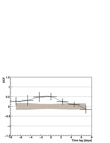
(a) RXTE vs. MAGIC & VERITAS

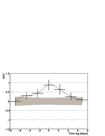
(b) RXTE vs. XRT

Figure 3: Discrete Correlation Function for time lags from -8 to +8 days in steps of $\sim 2$ days. The grey band represents the expected fluctuation of the DCF values in the case of completely uncorrelated time series given the error bars from the actual observations.

In order to study the multifrequency cross-correlations between the different energy bands we used the Discrete Correlation Function (DCF) as described in [13]. This method can also be applied in the case of unevenly sampled data as taken in this campaign.
The DCF was derived for all different combinations of instruments / energy regions and also for artificially introduced time lags (ranging from -8 to +8 days) between the individual light curves. Such time lags may occur as a result of spatially separated emission regions of the individual flux components (as expected, for example, in external inverse Compton models), or may be caused by the energy dependent cooling time-scales of the emitting electrons.
Based on the MWL data from this campaign, significant correlations have been found for the pairs RXTE/PCA - Swift/XRT and also (less significant) RXTE/PCA (or Swift/XRT) with MAGIC and VERITAS (Fig. 3a and 3b). In both cases, the DCF maximum is obtained for a zero time lag with a value of $0.87\pm 0.28$ (RXTE/PCA - Swift/XRT ) and $0.5\pm 0.19$ (RXTE/PCA - MAGIC and VERITAS) respectively. Due to the modest flux variability and / or large flux errors, no strong conclusions could be drawn from this analysis.

5 SED modeling

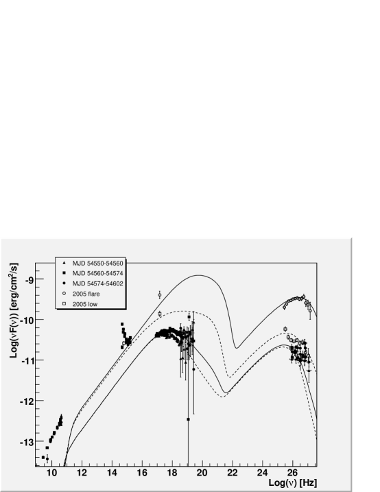
Figure 4: Broadband SED for Mrk 501 as obtained during this campaign in comparison to low and high states from 2005. The results from a SSC model fit to the low state 2008 data (dot-dashed cuve), the high state 2008 data (heavy-dashed curve), the 2005 low state (light-dashed curve) and the 2005 high state (solid line curve) are shown.

Table 1: The SSC model parameters used to describe the broadband SED for different flux states of the campaign.

	2008	2008	2005	2005
	high state	low state	high	low
$\gamma_{\mathrm{break}}$	$2.6\cdot 10^{5}$	$2.2\cdot 10^{5}$	$1.0\cdot 10^{6}$	$1.0\cdot 10^{5}$
n1	2.0	2.0	2.0	2.0
n2	3.9	4.2	3.9	3.2
B [G]	0.19	0.19	0.23	0.31
K [cm${}^{-3}]$	$1.8\cdot 10^{4}$	$1.8\cdot 10^{4}$	$7.5\cdot 10^{4}$	$4.3\cdot 10^{4}$
R [cm]	$3\cdot 10^{15}$	$3\cdot 10^{15}$	$1\cdot 10^{15}$	$1\cdot 10^{15}$
$\delta$	12	12	25	25

The broadband SED of Mrk 501 for the three different time periods defined above, together with some historical data from the 2005 low and high state of the object are shown in Fig. 4. The host galaxy contribution ($12.0\pm 0.3\ \mathrm{mJy}$ [14]) has been subtracted from the optical (KVA) data while the $\gamma$-ray spectra have been corrected for EBL absorption using the ‘low-IR’ model of [15]. The results from a one-zone SSC model fit to the different data sets are also shown in the figure as dashed lines. The model code was developed by Tavecchio et al. ([16, 7]) and is based on the following characteristic parameters: a spherical emission region with radius $R$ and Doppler factor $\delta$, a magnetic field of strength $B$, an electron distribution (density $K$) following a broken power law with slopes $n_{1}$ and $n_{2}$ and break energy $\gamma_{\mathrm{break}}$. The actual values of these model parameters for the two different emission states during the campaign and the historical data from 2005 are given in Tab. 1. As can be seen from Fig. 4 the model is able to accurately reproduce the data at X-ray energies. Given the relatively small differences in the SEDs of the two emission states of the campaign, only marginal changes of the model parameters were required in order to adjust the model to the two states. The proposed explanation for the low - high state transition is the injection of fresh, high-energy electrons which lead to a shift of the $\gamma_{\mathrm{break}}$ energy and to a hardening of the spectrum.
The discrepancy between the model and the data at lower energies (radio, optical) can be caused by synchrotron radiation from additional, cooler electron populations which could be present at different locations in the jet. The higher (than expected) fluxes at radio/optical frequencies were discussed in the past (also with Mrk501 data) in the framework of the helical-jets in blazar scenarios [17] or the blob-in-jet scenario [18]. As is shown in table 1, in comparison to the historical 2005 SED, the model parameters have changed significantly. However, it is worth noticing that the sparse coverage of the 2005 data allow for a lot of degeneracy among the (large) number of model parameters. A robust statement from the comparison of the 2005 and 2008 SEDs is that, while the X-ray and gamma-ray fluxes did change substantially between these two epochs, the fluxes at optical frequencies remained approximately the same. In the framework of two populations of electrons, this result suggests that the population of cool electrons does not vary with time while the population of electrons responsible for the X-ray (Synchrotron) and gamma-ray (Inverse Compton) emission is very dynamic. A more detailed modeling of the experimental data will be performed in a forthcoming publication [9].

References

- [1] J. Quinn, et al.1996, ApJ, 456, L831
- [2] F. Aharonian, et al.1999, A&A, 342, 69
- [3] E. Pian, et al.1998, ApJ, 492, L17
- [4] J. Albert, et al.2007, ApJ, 669, 862
- [5] J. Kataoka, et al.1999, ApJ, 514, 138
- [6] H. Krawczynski, et al.2000, A&A, 353, 97
- [7] F. Tavecchio, et al.2001, ApJ, 554, 725
- [8] H. Anderhub, et al.2009, submitted to ApJ
- [9] D. Paneque et al.2009, SLAC-PUB-13628, in preparation.
- [10] S. Vaughan, et al.2003, MNRAS, 345, 1271
- [11] K. Nandra, et al.1997, ApJ, 476, 70
- [12] R. Edelson, et al.2002, ApJ, 568, 610
- [13] R. Edelson and J. Krolik. 1988, ApJ, 333, 646
- [14] K. Nilsson, et al.2007, A&A, 475, 199
- [15] T. Kneiske, et al.2004, A&A, 413, 807
- [16] F. Tavecchio, et al.1998, ApJ, 509, 608
- [17] M. Villata and C.M. Raiteri 1999, A&A, 347,30
- [18] K. Katarzynski, et al.2001, A&A, 367,809