Applying Local Clustering Method to Improve the Running Speed of Ant Colony Optimization

Abstract

Ant Colony Optimization (ACO) has time complexity $O(tmN^{2})$, and its typical application is to solve Traveling Salesman Problem (TSP), where $t$, $m$, and $N$ denotes the iteration number, number of ants, number of cities respectively. Cutting down running time is one of study focuses, and one way is to decrease parameter $t$ and $N$, especially $N$. For this focus, the following method is presented in this paper. Firstly, design a novel clustering algorithm named Special Local Clustering algorithm (SLC), then apply it to classify all cities into compact classes, where compact class is the class that all cities in this class cluster tightly in a small region. Secondly, let ACO act on every class to get a local TSP route. Thirdly, all local TSP routes are jointed to form solution. Fourthly, the inaccuracy of solution caused by clustering is eliminated. Simulation shows that the presented method improves the running speed of ACO by 200 factors at least. And this high speed is benefit from two factors. One is that class has small size and parameter $N$ is cut down. The route length at every iteration step is convergent when ACO acts on compact class. The other factor is that, using the convergence of route length as termination criterion of ACO and parameter $t$ is cut down

I INTRODUCTION

I.1 Introduction of Ant Colony Optimization (ACO)

In 1991, Ant Colony Optimization (ACO) was presented firstly by M. DrigoA. Colorni11 and applied to solve TSP firstly by V. Mahiezzo et al.A. Colorni11 ; M Dorigo12 ; M Dorigo13 . Drigo et al. create a new research topic which is studied by many scholars now.

ACO is essentially a system based on agents that simulate the natural behavior of ants, in which real ants are able to find the shortest route from a food source to their nest, without using visual cues by exploiting pheromone informationM Dorigo13 . Pheromone is deposited when ants walking on a route. It provides heuristic information for other ants to choose their routes. The more dense the pheromone trail of a route is, the more possibly the route is selected by ants. At last, nearly all ants select the route that has the most dense pheromone trail, and it’s the shortest route potentially.

ACO has been applied to solve optimization problems widely and successfully, such as TSPA. Colorni11 ; M Dorigo12 ; M Dorigo13 ; Hai-Bin Duan14 , quadratic assignment problemManiezzo20 , image processingS. Meshoul24 , data miningRafael26 , classification or clustering analysisX. Li28 , biologyP. Meksangsouy29 . The application of ACO leads the theoretic study of ACO. Gutijahr firstly analyzes the convergence property of ACOW. J. Gutijahr36 . Stutzle & Dorigo prove the important conclusion, that if the running time of ACO is long enough, ACO can find optimal solution possiblyT Stuezle37 . The other interesting property is revealed currently by Birattari and et al. that the sequence of solutions of some algorithms does not depend on the scale of problem instanceMauro38 .

Running time is too long and the quality of solution is still low, that are the two main problems of ACO. To solve the main problems, the configuration of the parameters is discussedM Dorigo12 ; M Dorigo13 . The method of adaptation is used to improve ACOM Dorigo39 . Parallel computation and other method are used to accelerate ACOBullnheimer40 .

I.2 Clustering Correlates to the Running Time of ACO

One of study focus of ACO is to cut down running time. The running time of ACO is $O(t_{\max}MN^{2})$, and $M=[N/1.5]$ in general, where $t_{\max}$, $M$ and $N$ denote the iteration number, number of ants, and number of cities respectivelyHai-Bin Duan14 . The running time is proportional to $N^{2}$. Cutting down the number of cities $N$ is the key to reduce running time. Therefore, classifying all cities into different classes and letting ACO act on each class will reduce running time heavily. Hu and Huang used this method to improve the running speed of ACOXiao bing HU52 , which named ACO-K-Means. It’s faster than ACO by factors of 5-15 approximately. Simulations show that ACO-K-Means algorithm is valid only to the set of cities that has evident clustering feature, and invalid to more general situation. ACO-K-Means implies that it is possible that using clustering method to improve the running speed of ACO.

I.3 Introduction of Local Clustering Algorithm

Clustering is the classification of objects of a set (named training set) into different classes (or groups), so that the data in each class (ideally) share some common trait. One of most popular clustering algorithm is K-Means Clustering AlgorithmY. Linde47 ; Chao-Yang Pang48 . K-Means Clustering Algorithm assigns each point to the cluster whose center (i.e., centroid) is nearest to it, then update the centroid. Repeat this process until termination criterion is satisfied Chao-Yang Pang48 .

During the $t-th$ iteration of K-Means algorithm, the $i-th$ class has distortion that is defined as the average distance of each point and the class centroid, which is denoted by $D_{i}^{(t)}$ $(1\leq i\leq m)$, where $m$ is the number of classes. Pang proves that for each $i$, the distortion sequence $\{D_{i}^{(t)}\}$ is convergent if the $i-th$ class is separated from other classes evidently Chao-Yang Pang48 . That is, distortion sequence is convergent locally. According to this property, an algorithm named local clustering algorithm (LC) is presentedChao-Yang Pang49 , its essential idea is introduced as below.

Step1. K-Means is applied to a given training set to generate classes.

Step2. The class which distortion $D_{i}^{(t)}$ is convergent firstly is deleted from training set. Then update training set such that it is comprised by residual points. Go to step1.

Stop the process of step1-2 until all data is classified.

LC algorithm is faster than K-Means algorithm by factors of 4-13 approximately.

Suppose the $i-th$ class is $R_{i}^{(t)}$ during the $t-th$ iteration of K-Means algorithm. Set $R_{i}^{(t)}$ has entropy $H(R_{i}^{(t)})$, where $H(R_{i}^{(t)})=\underset{a\in R_{i}^{(t)}}{-\sum}p(a)\log_{2}p(a)$ and $p(a)$ is the probability of data $a$. It is proved that entropy sequence $\{H(R_{i}^{(0)}),H(R_{i}^{(1)}),\cdots,H(R_{i}^{(t)}),\cdots\}$ is convergent Chao-Yang Pang48 . That is, the convergent criterion of K-Means algorithm can be replaced by the convergence of entropy sequence Chao-Yang Pang50 . The K-Means with convergent criterion of entropy convergence is fast by two of factors at least Chao-Yang Pang50 ; Li X51 .

II IMPROVE LOCAL CLUSTERING ALGORITHM TO GENERATE COMPACT CLASS

II.1 Compact Set and The Method of Generation

For any subset of Euclidean space $R^{n}$, every sequence in this subset has a convergent subsequence, the limit point of which belongs to the set. This subset is called compact set. The conception of compact set (or compactness) is a topology conception. To understand it easily, compactness can be described visually as the phenomenon that many points cluster tightly in a small region, while non-compact set is the set that most of points clustering loosely in a big region.

K-Means Clustering, LC or other algorithm aim to partition a training set into classes. Some classes are compact and some are not. The most common situation is that a class contains a compact subset and some loose points, and the compact subset is around the center of the class. That is, the central part of class is compact possibly. To extract compact subset from a class, the following $3\delta$-principle is introduced.

For Gauss distribution, suppose that $\delta$ denotes the deviation of random data. It is the $3\delta$-principle that it’s more than 99% probability that a random point falling into the central region of data set which radius is $3\delta$ Chao-Yang Pang48 . The central region contains points more than 99%. Thus, if radius $3\delta$ is small enough and the number of points is big enough, the central region is compact. Even the central region with radius $3\delta$ is not compact, shortening the radius of central region to $\frac{3\delta}{4}$,$\ \frac{3\delta}{16}$, and so on will make it compact. For Gauss distribution which is comprised by enough points, the compact central region always exists. In general, for a class generated by clustering algorithm, all distances of points and class centroid comprise a gauss distribution approximatively. Therefore, the central region of a class is compact possibly.

Suppose the $i-th$ class is $R_{i}^{(t)}$ at the $t-th$ iteration of K-Means or LC algorithm. With the increase of iteration, class sequence $\{R_{i}^{(0)},R_{i}^{(1)},\cdots R_{i}^{(t)},R_{i}^{(t+1)}\cdots\}$ $(1\leq i\leq m)$ appears, where $m$ denotes the number of classes. Let

$$D_{i}^{(t)}=\frac{1}{\left|R_{i}^{(t)}\right|}\underset{x\epsilon R_{i}^{(t)}}{\sum}d(x,c_{i}^{(t)})$$ (1)

, where $\left|R_{i}^{(t)}\right|$ denotes the number of elements in $R_{i}^{(t)}$ and $d(x,c_{i}^{(t)})$ denotes distance.

$$\delta_{i}^{(t)}=\frac{1}{\left|R_{i}^{(t)}\right|}\underset{x\epsilon R_{i}^{(t)}}{\sum}\left|d(x,c_{i}^{(t)})-D_{i}^{(t)}\right|$$ (2)

Clearly, $D_{i}^{(t)}$ is the distortion of class $R_{i}^{(t)}$ and $\delta_{i}^{(t)}$ is the approximation of deviation of $D_{i}^{(t)}$.

$$K_{i}^{(t)}=\{x\mid d(x,c_{i}^{(t)})\leq\frac{1}{4^{p}}(D_{i}^{(t)}+3\delta_{i}^{(t)}),x\epsilon R_{i}^{(t)}(p\geq 0)\}$$ (3)

$K_{i}^{(t)}$ is the central region of class $R_{i}^{(t)}$. Parameter $p$ is used to shorten the radius of central region $K_{i}^{(t)}$ and makes it compact. Fig.1 illustrates the $3\delta$-principle and compact subset $K_{i}^{(t)}$.

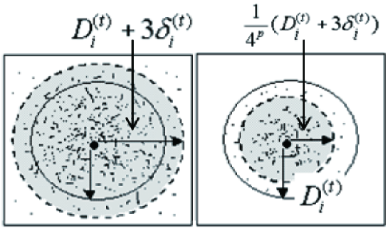
Figure 1: The illustration of compact central region of a class: In a class $R_{i}^{(t)}$, most of points cluster around their centroid and few points are far away from the centroid. Subset $K_{i}^{(t)}$ (i.e., the shadow part) is the central region of class $R_{i}^{(t)}$. Compact set is the set that many points cluster in a small region tightly. Increasing parameter $p$ will shorten radius and make $K_{i}^{(t)}$ compact.

II.2 Subroutine 1: Local Clustering Algorithm with $3\delta$-Principle

The local clustering algorithm with $3\delta$-principle is used to classify points into classes and to extract compact central region of classes. Its essential idea is described as below.

Firstly, apply LC algorithm to cluster data. And apply the criterion of entropy convergence (i.e.,$\frac{\left|H(R_{i}^{(t)})-H(R_{i}^{(t+1)})\right|}{H(R_{i}^{(t)})}\rightarrow 0$) to mark the stable class $R_{i}^{(t)}$.

Secondly, Extract compact central region $K_{i}^{(t)}$ from class $R_{i}^{(t)}$ and preserve it as a genuine class. Remove $R_{i}^{(t)}$ from training set and update it. Repeat above two steps until all compact central regions are extracted. The detail is described as below.

Input parameters:

$T$: Training Set

$m$: The number of class

$\varepsilon$: The stop threshold for clustering.

$C^{(0)}=\{c_{i}^{(0)}(1\leq i\leq m)$: Initial centroids set.

$p$: A parameter to adjust the size of compact subsets $K_{i}^{(t)}(p\geq 0)$.

Output:

$\varphi(T)=\{K_{1}^{(t)},K_{2}^{(t)},\cdots,K_{i}^{(t)},\cdots K_{m}^{(t)}\}$ (i.e., the set of compact subset, see fig.1)

$\sigma(T)=\{B_{1}^{(t)},B_{2}^{(t)},\cdots,B_{i}^{(t)},\cdots B_{m}^{(t)}\}$, where $B_{i}^{(t)}=R_{i}^{(t)}-K_{i}^{(t)}$, and it is comprised by dispersive points ( $1\leq i\leq m$, see fig.1)

void Subroutine1 ( $T$,$m$,$\varepsilon$,$C^{(0)}$,$p$,$\varphi(T)$,$\sigma(T)$)

{

Step1. Initialization: Let iteration number $t=0$. Let $Counter=m$. Let $\varphi(T)=\phi$ and $\sigma(T)=\phi$, where $\phi$ denotes empty set. According to initial centroids set $C^{(0)}$, generate initial partition of training set $\varphi^{(0)}=\{R_{i}^{(0)}\mid R_{i}^{(0)}\subset T,1\leq i\leq m\}$.

Step2. While ($Counter>0$)  {

Step2.1. Generate new centroids set $\ C^{(t+1)}=\{c_{i}^{(t+1)}\mid 1\leq i\leq m)\}$  and new partition $\varphi^{(t+1)}=\{R_{i}^{(t+1)}\mid 1\leq i\leq m\}$

/* Note: Check whether entropy sequence $\{H(R_{i}^{(0)}),H(R_{i}^{(1)}),\cdots,H(R_{i}^{(t)}),\cdots\}$ is convergent. If it is convergent, let the convergent marker $StableMarker(R_{i}^{(t+1)})=True$*/

Step2.2. For ($i=1$; $i\leq Counter$; i++)  {

Estimate the entropy of class $R_{i}^{(t+1)}$, i.e., $H(R_{i}^{(t+1)})=\log_{2}\left|R_{i}^{(t+1)}\right|$.

If ($\frac{\left|H(R_{i}^{(t)})-H(R_{i}^{(t+1)})\right|}{H(R_{i}^{(t)})}<\varepsilon$)  { $StableMarker(R_{i}^{(t+1)})=True$; }

else {$StableMarker(R_{i}^{(t+1)})=False$}

}

/*Note: Extract the data around the centroid of class as a genuine class */

Step2.3. For ($i=1$; $i\leq Counter$; i++)  {

If ($StableMarker(R_{i}^{(t+1)})=True$)  {

Calculate compact central region $K_{i}^{(t)}$ according to formula (3)

Calculate $B_{i}^{(t)}$: $B_{i}^{(t)}=R_{i}^{(t+1)}-K_{i}^{(t)}$

Let $\varphi(T)=\varphi(T)\cup K_{i}^{(t)}$

Let $\sigma(T)=\sigma(T)\cup B_{i}^{(t)}$

Update Training Set: $T=T-R_{i}^{(t)}$

Update centroids set: $C^{(t+1)}=C^{(t+1)}-\{c_{i}^{(t+1)}\}$

${\small\ \ \ \ \ \ \ \ Counter=Counter-1}$

}

}

$\ \ t=t+1$.

}

}

II.3 Special LC Algorithm to Generate Compact Classes (SLC)

Note that above subroutine 1 is not a partition of training set. Subroutine 1 extracts only compact central regions of all classes and the residual points are unclassified. The residual points comprise a new training set. And it’s possible that some of residual points cluster together tightly and comprise some small compact subsets again. These small compact subsets are new classes. To obtain these new classes and classify all points, SLC algorithm is described as below.

Input parameters:

$T_{0}$: Training Set

$m_{0}$: The initial number of classes.

$\varepsilon$: The stop threshold for clustering.

Output:

$Num$: The final number of classes.

$CLS$: The partition of $T_{0}$, in which each class is compact.

SLC Algorithm:

Step1. Initialization: Let $T=T_{0}$, $m=m_{0}$, $CLS=\phi$, and $p=0$.

Step2. For (i=0;$i<[\log_{2}m]$; i++)  /*Note: $[\log_{2}m]$ denotes the integer*/

{ Step2.1 Generate initial centroids set $\ C^{(0)}=\{c_{i}^{(0)}\mid 1\leq i\leq m)\}$.

Step2.2 Call Subroutine1 ( $T$,$m$,$\varepsilon$,$C^{(0)}$,$p$,$\varphi(T)$,$\sigma(T)$)

Step2.3 $CLS=CLS\cup\varphi(T)$;

Step2.4 $T=\sigma(T)$;

/*Note: Increase $p$ to get smaller compact class*/

Step2.5 $m=[\frac{m}{2}]$; $p=p+1$;

}

Step3 Every residual point $x$ in the last set $\sigma(T)$ is regarded as a class $\{x\}$. And let $CLS=CLS\cup\{x\}$. Let $Num$ denote the number of classes contained in $CLS$. The two outputs are $CLS$ and $Num$.

II.4 The Clustering for Mixture Distribution (SLC-Mixture)

The clustering algorithm SLC presented above generates spherical classes only. However, for a general distribution, some classes are spherical shape, some classes are chain shape in which points cluster closely around a curve (or a line), even some classes contain isolated points. This common distribution is called mixture distribution. For a large-scale TSP, the distribution of cities is mixture distribution in general. The clustering method for mixture distribution is proposed as below.

II.4.1 The Simple Maker to Distinguish Spherical Class from Chain-Shaped Class

The position of city on a map is two-dimensional point. A given class can be divided into 8 areas along the 4 directions of the north-south, west-east and two diagonal lines through the centroid of the class. If the class is spherical, the percentage of points in each area is close to 1/8 and is the same approximately. If the class is chain-shaped class (or part of chain-shaped class), it’s impossible that the percentage of every area is close to 1/8 at the same time. Therefore, the percentage of points in each area is the maker of spherical class. Fig.2 illustrates the marker.

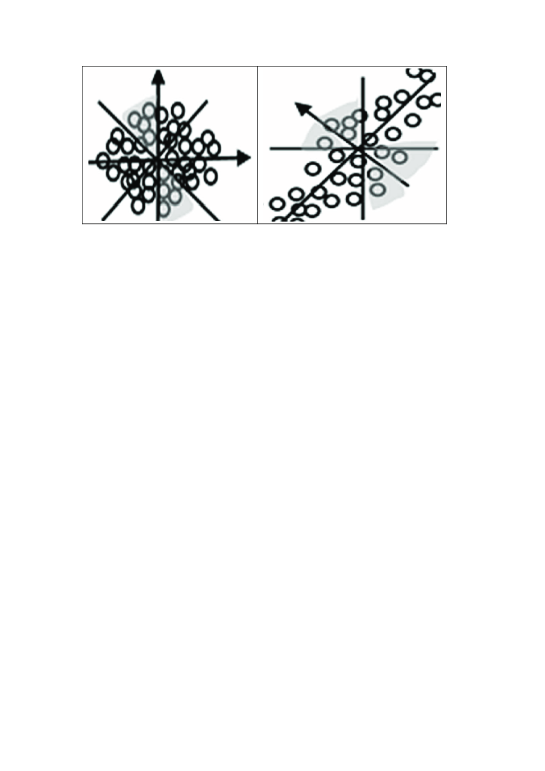
Figure 2: The Illustration of Distinguishing Spherical Class from Chain-shaped Class: A given class is divide into 8 parts along the 8 lines through the centroid of the class. If the class is spherical, the percentage of each part is close to threshold $\epsilon=1/8$. If the class is chain-shaped class (or part of chain-shaped class), there are 2-4 parts which percentage is far less than 1/8. Therefore, the percentage of each part is the marker of spherical class. $\varepsilon=0.058$ in this paper because some classes are elliptical.

II.4.2 Applying SLC to Process Mixture Distribution (SLC-Mixture)

At first, apply SLC to classify all data of training set. Secondly, apply the marker presented above to distinguish spherical classes and extract them from the training set. Then all residual points comprise a new set named residual set. The residual set contains only chain-shaped classes and isolated points. Third, apply the method presented in Ref.HUANG Xiaobin53 to classify all residual points of residual set into different chain-shaped classes or marked as isolated points. The method presented in Ref.HUANG Xiaobin53 is named Chain-Shaped Clustering Algorithm and is introduced at appendix I.

The clustering method presented in this section is called SLC-Mixture algorithm, which processes the mixture distribution of spherical classes, chain-shaped classes and isolated points.

III APPLY SLC TO ACO  

III.1 The Termination Criterion of ACO

Suppose ACO acts on a compact class and let $L_{t}$ denotes the minimum route length that is generated at the $t-th$ iteration of computation. There are sequence $\{L_{1},L_{2},\cdots,L_{t},L_{t+1},\cdots\}$ and it is convergent under idea condition. The convergent criterion $\frac{\left|L_{t}-L_{t+1}\right|}{L_{t}}\leq\varepsilon$ is proposed as the termination criterion of ACO in this paper.

In the following discussion, ACO refers to the algorithm which termination criterion is $(\left|L_{t}-L_{t+1}\right|/L_{t})\leq\varepsilon$.

III.2 Apply SLC to Improve The Running Speed of ACO (ACO-SLC)

In this section, the clustering algorithm SLC will be applied to improve the running speed of ACO. The method is named ACO-SLC and it is described as below.

Input Parameter:

$T$: Set of cities

Output:  The shortest TSP route obtained by the algorithm

ACO-SLC Algorithm:  

Step1. Apply SLC algorithm to partition set $T$. The classes are $B_{1},B_{2},\cdots,B_{i},\cdots B_{Num}$, and their centroids are $b_{1},b_{2},\cdots,b_{i},\cdots b_{Num}$ respectively.

Stpe2. Construct graph $G^{{}^{\prime}}$: Centroids $b_{1},b_{2},\cdots,b_{i},\cdots b_{Num}$ are regarded as virtual cities respectively, and the virtual cities are regarded as the vertices of graph $G^{{}^{\prime}}$. For a pair of classes $B_{i}$ and $B_{j}$, if there exists two cities that belong to $B_{i}$ and $B_{j}$ respectively and they joint each other, use an edge to joint the two corresponding vertices $b_{i}$ and $b_{j}$. The weight of edge is the minimum distance between two classes, i.e.,

$${\small d(B}_{i}{\small,B}_{j}{\small)=}\min{\small\{d(x}_{i}{\small,x}_{j}{\small)\mid x}_{i}{\small\epsilon B}_{i}{\small,x}_{j}{\small\epsilon B}_{j}{\small\}}$$ (4)

Step3. Calculate a TSP route of graph $G^{{}^{\prime}}$ to generate the traveling order of all classes: Let ACO algorithm act on graph $G^{{}^{\prime}}$ to find a TSP route denoted by $b_{j_{1}},b_{j_{2}},\cdots b_{j_{Num}}$, where $j_{1},j_{2},\cdots j_{Num}$, is a permutation of sequence $1,2,\cdots Num$. The pair of classes $B_{j_{i}}$ and $B_{j_{(i+1)}}$ is called neighbor class.

Step4. Choose an edge as the bridge to joint a pair of neighbor classes, and this edge is named bridge edge: Assume that the two neighbor classes are $B_{j_{1}}$ and $B_{j_{2}}$. If there exist an edge such that

$${\small d(x}_{u}{\small,x}_{v}{\small)=}\min{\small\{d(a,b)\mid a\epsilon B}_{j_{1}}{\small,b\epsilon B}_{j_{2}}{\small\}}$$ (5)

, edge $(x_{u},x_{v})$ is the bridge edge, $x_{u}$ and $x_{v}$ are called border cities, where vertices $a$ and $b$ should be not used to joint other neighbor classes.

Step5. Calculate a local TSP route for every class $B_{i}(1\leq i\leq Num)$: Add a new edge to joint the two border cities in the class, and mark the edge as necessary edge of the local TSP route. This edge is named pseudo-edge. Let the ACO algorithm with convergence criterion $(\left|L_{t}-L_{t+1}\right|/L_{t})\leq\varepsilon$ act on the class to generate a local TSP route.

Step6. Construct a TSP route: Walk along the traveling order obtained at step3, for every pair of neighbor classes, delete the pseudo-edge of each class such that the local route is not close. Then let the local route of each class and the bridge edge between these two classes be jointed.

Fig.3 illustrates the processing of ACO-SLC algorithm.

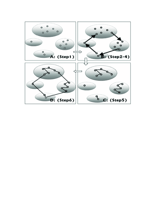
Figure 3: The schematic diagram of ACO-SLC : Firstly, classify all points into compact classes. Secondly, the centroid of each class is regarded as a virtual city, and calculate a virtual TSP route. Then along the virtual route, joint all classes. Thirdly, let ACO act on each class to get a local TSP route. Fourthly, joint all local TSP routes along the virtual route to form the last route.

III.3 Using the Method of Little-window and Removing Cross-edge to Improve ACO-SLC (ACO-SLC-LWCR)

Clustering may cause the error of solution although it improves the running speed of ACO heavily. If all classes are compact and separated clearly, the quality of solution of ACO-SLC should be very good. However, in fact, the border between two neighbor classes is fuzzy. The fuzzy border will cause the inaccuracy of solution, and much longer route will appear. And recognizing the longer part and removing it will generate better solution possibly. It is well known that, the shortest route is always at the surface of a convex hull. Thus, the longer part should be at the inner of a convex hull and two longer edges intersect. In other words, intersection of two edges is a marker of longer part of a route possibly. According to the marker, removing longer edges is call removing cross-edge or removing intersection edges, which is similar to the method in Hai-Bin Duan14 . (Notice: in Ref.Hai-Bin Duan14 , before execute ACO, the long and crossed edges are removed to improve the running speed of ACO, not to improve the solution quality.)

Fig.4 illustrates the method of removing cross-edge.

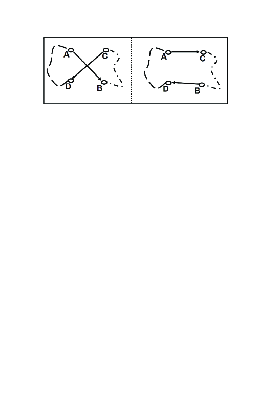
Figure 4: The Illustration of Removing Cross-edges from TSP Route: At the left figure, $AB$ and $CD$ intersect each other. There is a principle that shortest route is at the surface of a convex hull. Thus, edge $AB$ and $CD$ is the longer part of route and should be removed. Removing these two edges will generate shorter route (see right figure).

In addition, a simple method named little-window strategy is proposed to improve the running speed of ACO in Ref.XIAO46 . Construct a set $S_{i}$ that is comprised by $w$ accessible and short edges which join the $i-th$ city, where $w$ is a pre-assigned constant. The ant which has arrived at $i-th$ city will select an edge from window set $S_{i}$ only to arrive its next city, and not selection an edge from all neighbor edges of this vertex. So, this method improve the running speed of ACO. In addition, the parameter configuration of the method is put at appendix II.

The ACO-SLC with little-window strategy and cross-edges removing is called ACO-SLC-LWCR.

III.4 The ACO-SLC for Mixture Distribution (ACO-SLC-Mixture)

ACO-SLC is suitable for the spherical shape distribution only, and the low quality of solution will appear possibly when ACO-SLC is applied to process mixture distribution. To process mixture distribution, the following method named ACO-SLC-Mixture is proposed in this paper.

Firstly, apply SLC-Mixture at section 2.4.2 to partition the set of cities into spherical classes, chain-shaped classes, or isolated points. Secondly, apply ACO-SLC-LWCR to each class and generate a TSP route.

IV SIMULATION

In this section, five related algorithms ACO, ACO-K-Means, ACO-SLC, ACO-SLC-LWCR, ACO-SLC-Mixture are tested and compared. In the following simulation, ACO refers to Ant-cycle presented by Dorigo, which is very typical A. Colorni11 .

All test data in this paper is downloaded from http://www.iwr. uniheidelberg.de /iwr/comopt/soft /TSPLIB95/TSPLIB.html. All algorithms in this paper run on personal computer. CPU: 1.80GHz. Memory: 480M. Software: Matlab. The parameters are listed as below. Initialize pheromone trails $\tau_{ij}(0)=1$, iteration number $1000$, $\varepsilon=0.001$, $\alpha=1$, $\beta=10$, $\rho=0.4$, $Q=300$, $m=[\frac{N}{1.5}]$. Two performance items are tested. One item is the running time, which is defined as $Ratio=Time(ACO)/Time(Algorithm)$. The bigger the ratio is, the faster the algorithm is. The other item is the quality of solution, which is defined as the percentage of error $Error=(Solution-Optimum)/Optimum$, where $Optimum$ denotes the best solution known currently. The smaller the error is, the better the quality of solution is.

The performances of the five algorithms are listed in Fig.5. It shows that ACO-SLC, ACO-SLC-LWCR and ACO-SLC-Mixture are faster than ACO by 415~10736, 390~10192 and 257-9419 of factors respectively! However, some solutions of ACO-K-Means and ACO-SLC have low quality. The inaccuracy ratio of ACO-SLC-Mixture is less than ACO in most cases, and is bigger than ACO by 2% at most.

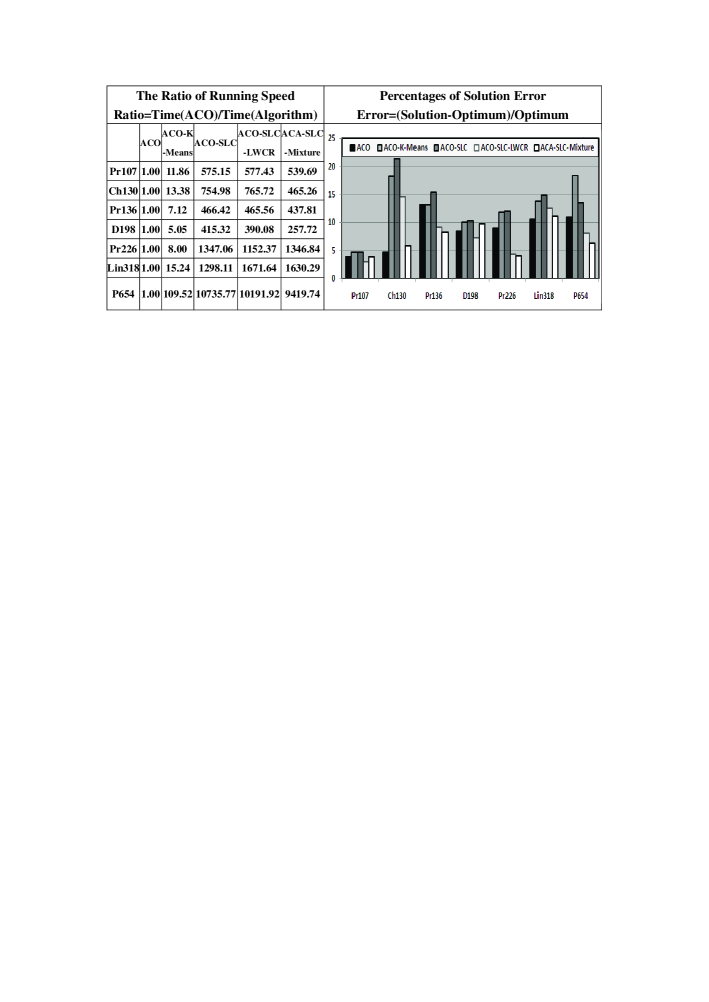
Figure 5: The Performance Comparison of The Five Algorithms of ACO, ACO-K-Means, ACO-SLC ACO-SLC-LWCR and ACO-SLC-Mixture: The figure shows that ACO-SLC algorithm, ACO-SLC, ACO-SLC-LWCR and ACO-SLC-Mixture are faster than ACO by 415~10736, 390~10192 and 257-9419 of factors respectively! However, some solutions of ACO-K-Means and ACO-SLC have low quality. ACO-SLC-Mixture can process mixture distribution and its inaccuracy ratio is less than ACO in most cases, and is bigger than ACO by 2% at most.

The Defect of ACO-SLC: The authors have done many simulations under different conditions. And these simulations show the quality of ACO-SLC solution depends on the quality of clustering and clustering quality of SLC is sensitive to the initial centroids just liking K-Mean algorithm. This is main defect of ACO-SLC. All cities are two-dimensional (or three-dimensional) points and they are visual for general TSP problems. Hence, reasonable initial centroids can be selected by researcher’s eyes to reduce the sensitivity of initial centroids. The initial centroids of the simulations of this paper is selected by the authors’ eyes, and they are put at appendix III of this paper.

V CONCLUSION

Time Complexity of ACO: ACO is the algorithm that inspired by the foraging behavior of ant colonies and has be applied to solve many optimization problem. The typical application of ACO is the application at Traveling Salesman Problem (TSP). The running time of ACO is $O(t_{\max}MN^{2})$, where $t_{\max}$, $M$ and $N$ denotes the iteration number, number of ants, and number of cities respectively. Parameter $m$ is a experiential value and is set to $[\frac{N}{1.5}]$ in general. Parameter $N$ is the key factor of running time because running time is proportional to its square. Parameter $t_{\max}$ and $N$ are available, and decreseaing parameter $t_{\max}$ and $N$ will cut down running time.

Focus of ACO Study: ACO can generate solution with high quality in general. But its shortage is that running time is too long. Cutting down running time is one of study focuses of ACO, and one way is to decrease parameter $t_{\max}$ and $N$, especially $N$.

Basic Idea for This Study Focus: For this study focus, the following basic idea is presented in this paper.

Firstly, all cities are classified into compact classes, where compact class is the class that all cities in this class cluster tightly in a small region.

Secondly, let ACO act on every class to get a local TSP route.

Thirdly, all local TSP routes are jointed to form solution.

Fourthly, the inaccuracy of solution caused by clustering is eliminated.

Realization of Basic Idea: The realization of above idea is based on a novel clustering algorithm presented in this paper, which is named Special Local Clustering algorithm (SLC). The running time of SLC is far less than the time of ACO. SLC generates compact classes, while current popular clustering algorithm such as K-Means does not generate compact classes in general. The compactness of class makes the length of TSP route $L_{t}$ at every iteration convergent, the convergence of $L_{t}$ (i.e., $(\left|L_{t}-L_{t+1}\right|/L_{t})\rightarrow 0$) is proposed as the termination criterion of ACO in this paper. Thus, parameter $t_{\max}$ is cut down to improve the running speed of ACO. In addition, every class has small size, ACO acting on small class makes parameter $N$ is cut down, and running speed is improved. According to this analysis, ACO-SLC algorithm is presented in this paper. Simulation shows that ACO-SLC is faster than ACO by 415~10736 of factors!

Elimination of the Solution Inaccuracy Caused by Clustering: Although the running speed is improved in this paper, the inaccuracy of solution is heavy. Two factors causing the inaccuracy are found in this paper. One is the cross-edges (see section 3.3), and the other factor is the unmatch between ACO-SLC and mixture distribution (see section 3.4). According to these two factors, ACO-SLC-LWCR and ACO-SLC-Mixture are presented in this paper, which is the improvement of ACO-SLC. Simulation shows that ACO-SLC-LWCR and ACO-SLC-Mixture is faster than ACO by 390~10192 and 257-9419 of factors respectively! The inaccuracy ratio of ACO-SLC-Mixture is less than ACO in most cases, and is bigger than ACO by 2% at most.

VI ACKNOWLEDGMENT

The authors appreciate the help from Prof. J. Zhang, Prof. J. Zhou and Prof. Qi Li. The authors would like to thank group members Mr. C.-B. Wang and Ms. Q. Yang for their check.

VII APPENDIX

Appendix I: Chain-Shaped Clustering Algorithm of Ref.HUANG Xiaobin53

This algorithm is used to process the data set which distribution is chain-shaped only, and is introduced as below.

Step1. Unify all data and calculate the centroid of data set, and select the point that is farthest from the centroid as the seed of the first class.

Step2. Select the points that are close to the seed into the first class as many as possible until the trace of the first set is bigger than the pre-assigned threshold (Notice: The set of random data has covariance matrix. The trace of covariance matrix is proportion to the size of region containing these random data. The smaller the trace is, the smaller the size is. Thus, if the trace is less than a pre-assigned threshold, the class is still small and compact. The threshold is 0.0005 in this paper).

Repeating the two steps, the first class, second class, 3rd class, and so on, will be obtained until all points are classified. Finally, merge all neighbor classes as a new big class. E.g., if class A is close to B and B close to C the three classes A, B and C are neighbors and are merged as a big chain-shaped class.

Appendix II: The Parameter Configuration of Little-Window Method

The configuration of parameter $w$ in little-window strategy: Let $n$ denotes the number of neighbor cities, If $n<21$, let w=min($n$-1, 8); Else if $n<101$, let w=min($n$-1, 9); Else if $n<144$, let w=min($n$-1,13); Else if $n<1000$, let w=min($n$-1, 19); Else $ifn<4000$, let w=min($n$-1,100); Else let $w=[n/10]$;

Appendix III: Initial Centroids of Classes

The initial centroids of classes which is used by clustering algorithm SLC: Each initial centroids has coordinate (x, y)

Pr136 x= 5000 5000 5000 5000  12000 12000 12000 12000 y= 3000 5000 8000 10000 10000 8000  5000  3000 Pr226 x= 550  4800 4800 2000 4000  12000 12500 10000 12500 16500 13000 8800 y= 2000 7000 9000 9000 12000 12000 8500  8500  7000  3500  2000  3500 Ch130 x= 50 90  90  40  40  150 300 200 270 200 260 400 400 450 550 400 560 700 700 700 y= 50 190 340 450 680 100 50  250 400 540 650 50  150 300 200 540 400 200 380 550 Lin318 x= 500 500  500  500  1400 1400 1400 1100 2300 2300 2300 2000 3000 3000 3000  3000 y= 500 1500 3100 4000 500  1800 3200 4000 500  1700 3100 4000 500  1500  2700 3600 D198 x= 3700 3670 3830 3800 3700 4000 2100 1800 1600 1300 950  700  0 1500 1160 1500 1600 2100 y= 1400 1400 1400 1150 1050 1050 1870 1600 1480 1400 1350 1000 0 1000 1170 1190 1400 1400 P654 x= 1070 1070 1070 1500 1070 1070 1070 1070 2000 2500 2000 3500 4300 4500 5840 5840 5840 5840 5840 5840 y= 2400 2200 2710 3600 4800 4500 5050 5200 2500 4000 5000 3500 3500 2400 2200 2710 2700 4900 4600 5300 Pr107 x= 8500 8500 8500 8500 8500 8500 8500 8500  8500  16000 16000 16000 16000 16000 16000 16000 16000 16000 y= 4800 5500 6400 7100 8000 8900 9800 10600 11500 4800  5500  6400  7100  8000  8900  9800  10600 11500

References

- (1) M. Birattari, P. Pellegrini, and M. Dorigo, “On the Invariance of Ant Colony Optimization,” IEEE TRANSACTIONS ON EVOLUTIONARY COMPUTATION 11 (2007) 732-742.
- (2) B. Bullnheimer, R. F. Hartl,and C. Strauss, “New Rank Based Version of the Ant System A Computational Study,” A Computational Study Technical report, University of Viena, Institute of Management Science, pp. 1-16, 1997, http://citeseer.ist.psu.edu/166666.html.
- (3) C. Blum , M. Dorigo “The hyper-cube framework for ant colony algorithm,” IEEE Trans. on SMC 34 (2004) 1161-1172.
- (4) B. Bullnheimer, G. Kotsis, and C. Steauss “Parallelization strategies for the ant system,” High Performance and Algorithms and Software in Nonlinear Optimization, Applied Optimization 24 (1998) 87-100.
- (5) Y. Chen, Y. Pan, L. Chen, J. Chen, “Partitioned optimization algorithms for multiple sequence alignment,” 20th International Conference on Advanced Information Networking and Applications - Volume 2 (AINA’06) , Los Alamitos, CA, USA, 2006, pp. 618-622.
- (6) D. Chu, M. Till, A. Zomaya, “Parallel Ant Colony Optimization for 3D Protein Structure Prediction using the HP Lattice Model,” Proc 19th IEEE International Parallel and Distributed Processing Symposium-Vol.7, Los Alamitos, CA, USA, 2005, pp. 1-7.
- (7) A. Colorni, M. Dorigo, and V. Maniezzo, “Distributed optimization by ant colonies,” In Proceedings of the 1st European Conference on Artificial Life, Paris, France, 1991, pp. 134-142,
- (8) O. Cordon, I. Viana, F. Herrera, L. Moreno , “A new ACO model integrating evolutionary computation concepts: the best-worst ant system,” Proceedings of the 2nd Inernational Workshop on Ant Algorithm/ANTS2000, Brussels, Belgiums, 2000, pp. 22-29.
- (9) M. Dorigo, L. M. Gambardella, “study of Ant-Q,” Proceedings of 4th International Conference on Parallel Problem from Nature,Berlin, 1996, pp. 656-665.
- (10) M. Dorigo, L. M. Gambardella, “Ant colony system: A cooperative learning approach to the traveling salesman problem,” IEEE Trans. on Evolutionary Computation 1 (1997) 53-66
- (11) M. Dorigo, V. Maniezzo, and A. Colorni, “Ant system: Optimization by a colony cooperating Agents,” IEEE Trans. on Systems, Man, and Cybernetics Part B: Cybernetics, 26 (1996) 29-41
- (12) Hai-Bin Duan, ANT COLONY ALGORITHMS: THEORY AND APPLICATIONS, Science Publisher, Beijin, China, 2005.
- (13) L. M. Gambardella, Marco Dorigo, “Ant-Q: A Reinforcement Learning approach to the traveling salesman problem,” Proceedings of ML-95, Twelfth Intern. Conf. on Machine Learning, Morgan Kaufmann, 1995, pp. 252-260.
- (14) L.M. Gambardella, M. Dorigo, “Solving symmetric and asymmetric TSPs by ant colonies,” IEEE Conference on Evolutionary Computation (ICEC’96), Nagoya, Japan, 1996, pp. 622-627.
- (15) W. J. Gutijahr, “A generalized convergence result for the graph based ant system.” Technical Report 99-09, Dpet. Of Statistics and Decision Support Systems, Univ. of Vienna, Austria, 1999.
- (16) W. J. Gutijahr, “A graph-based ant system and its convergence,” Future Generation Computer Systems 16 (2000) 873-888.
- (17) N. Holden, A. Freitas, “Hierarchical Classification of G-Protein-Coupled Receptors with a PSO/ACO Algorithm,” Proc. of the 2006 IEEE Swarm Intelligence Symposium,Indianapolis, Indiana, USA, 2006, pp.77-84, http://www.cs.kent.ac.uk/people/staff/aaf/pub_papers.dir/IEEE-SIS-2006-Holden.pdf.
- (18) Xiao bing HU and Xi yue HUANG, “Solving tsp with characteristic of clustering by ant colony algorithm,” Journal Of System Simulation 16 (2004) 55-58.
- (19) HUANG Xiaobin, WANG Jianwei and ZHANG Yan, “Adaptive K Near Neighbor Clustering Algorithm for Data with Non-spherical-shape Distribution,” Computer Engineering 29 (2003) 21-22.
- (20) X. Li , X.- H. LUO , and J.- H. ZHANG. “Codebook design by a hybridization of ant colony with improved LBG algorithm,” IEEE Int. Conf. Neural Networks and Signal Processing, Nanjing, China, 2003, pp.469-472.
- (21) LI Xia LUO Xuehui ZHANG Jihong. “Modeling of Vector Quantization Image Coding in an Ant Colony System,” Chinese of Journal Electronics 13 (2004) 305-307.
- (22) Y. Linde, A. Buzo, and R. M. Gray, “An algorithm for vector quantization design,” IEEE Trans on.Commum COM-28 (1980) 84-95.
- (23) V. Maniezzo, V. Colorni, A., “The ant system applied to the quadratic assignment problem,” IEEE Transactions on Knowledge and Data Engineering 11 (1999) 769-778.
- (24) V. Maniezzo, “Exact and approximate nondeterministic tree-search procedures for the quadratic assignment problem,” INFORMS Journal on Computing 11 (1999) 358-369, http://www.amitkoth.com/weblog/dissertation/documents/maniezzo98exact.pdf.
- (25) D. Martens, M. Backer, R. Haesen, J. Vanthienen, M. Snoeck, and B. Baesens, “Classification With Ant Colony Optimization,” IEEE TRANSACTIONS ON EVOLUTIONARY COMPUTATION 11 (2000) 651-665.
- (26) P. Meksangsouy, N. Chaiyaratana, “DNA fragment assembly using an ant colony system algorithm,” Proceedings of the 2003 Congress on Evolutionary Computation, Canberra, Australia, 2003, pp. 1756-1763.
- (27) D. Merkle, M. Middendorf “Fast ant colony optimization on runtime Reconfigurable processor arrays,” Genetic Programming and Evolvable Machine 3 (2002) 345-361
- (28) P. Merz, B. Freisleben, “Fitness landscape analysis and memetic algorithms for the quadratic assignment problem,” IEEE Transactions on Evolutionary Computation 4 (2000) 337-352.
- (29) S. Meshoul, M. Batouche, “Ant Colony System with Extremal Dynamics for Point Matching and Pose Estimation,” Proceeding of the 16th International Conference on Pattern Recognition, Quebec, 2002, pp. 823-826.
- (30) J. Moss and G. Johnson, “An ant colony algorithm for multiple sequence alignment in bioinformatics,” Artificial Neural Networks and Genetic Algorithms, Springer, April 2003, pages 182-186, http://www.cs.kent.ac.uk/pubs/2003/1707/content.pdf.
- (31) Chao-Yang Pang, “Vector Quantization and Image Compression,” Doctoral thesis, University of Electronic Science and Technology of China, Chengdu, China, Jun 2002.
- (32) Pang Chaoyang, Sun Shixin, Pan Ye, and Gong Haiying, “A fast codebook training algorithm using local clustering,” Journal of Electronics and Information Technology 9 (2002) 1282-1286
- (33) PANG Chao-yang and SUN Shi-xin, “Codebook trainning algorithm by the convergence of entropy sequence tor vector quantization,” Systems Engineering and Electronics 24 (2002) 83-85.
- (34) Rafael S. Parpinelli, Heitor S. Lopes, “Data Mining With an Ant Colony Optimization Algorithm,” IEEE Transactions on Evolutionary Computation 6 (2002) 321-332.
- (35) D. Piriyakumar, P. Levi “A new approach to exploiting parallelism in ant colony algorithm,” In: International Symposium on Micromechatronics and Human Science (MHS), Nagoya, Japan, 2002, pp. 237-243.
- (36) M. Randall , A. Lewis “A parallel implementation of ant colony algorithm,” Parallel and Distributed Computing 62 (2002) 1421-1432.
- (37) A. Shmygelska and H. Hoos, “An ant colony optimisation algorithm for the 2D and 3D hydrophobic polar protein folding problem,BMC Bioinformatics ” 6 (2005) 30-, http://www.biomedcentral.com/1471-2105/6/30.
- (38) T. Stutzle, M Dorigo, “ACO algorithms for the quadratic assignment problem,” New Ideas in Optimization, McGraw-Hill Inc., US, 1999. http://neo.lcc.uma.es/EAWebSite/SKELETON/ANT/BC.05-StuDor-NIO99.pdf.gz.
- (39) T. Stutzle, M Dorigo, “A short convergence proof for a class of ant colony optimization algorithms,” IEEE Trans. On Evolutionary Computation 6 (2002) 358-365.
- (40) T. Stutzle, H. Hoos, “MAX-MIN Ant System,” Future Generation Computer Systems 16 (2000) 889–914. http://www.cs.ubc.ca/spider/hoos/Publ/fgcs00.ps.gz.
- (41) E. Talbi, O. Roux , C. Fonlupt, D. Robilard “Parallel ant colonies for the quadratic assignment problem,” Future Generation Computer Systems 17 (2001) 441-449.
- (42) XIAO Yunshi, LI Bingyu, “Ant Colony Algorithm Based on Little Window,” Computer Engineering 29 (2003) 143-145.
- (43) H. Zheng, A. Wong, S. Nahavandi, “Hybrid ant colony algorithm for texture classification,” Proceeding of 2003 Congress on Evolutionary Computation-Vol.4, Washington, DC,USA, 2003, pp. 2648-2652.