Biological invasions: deriving the regions at risk from partial measurements

Abstract

We consider the problem of forecasting the regions at higher risk for newly introduced invasive species. Favourable and unfavourable regions may indeed not be known a priori, especially for exotic species whose hosts in native range and newly-colonised areas can be different. Assuming that the species is modelled by a logistic-like reaction-diffusion equation, we prove that the spatial arrangement of the favourable and unfavourable regions can theoretically be determined using only partial measurements of the population density: 1) a local “spatio-temporal” measurement, during a short time period and, 2) a “spatial” measurement in the whole region susceptible to colonisation. We then present a stochastic algorithm which is proved analytically, and then on several numerical examples, to be effective in deriving these regions.

Keywords: reaction-diffusion $\cdot$ biological invasions $\cdot$ inverse problem $\cdot$ habitat configuration $\cdot$ Carleman estimates $\cdot$ simulated annealing

1 Introduction

Because of trade globalisation, a substantial increase in biological invasions has been observed over the last decades (e.g. Liebhold et al. [1]). These invasive species are, by definition [2], likely to cause economic or environmental harm or harm to human health. Thus, it is a major concern to forecast, at the beginning of an invasion, the areas which will be more or less infested by the species.

Because of their exotic nature, invading species generally face little competition or predation. They are therefore well adapted to modelling via single-species models.

Reaction-diffusion models have proved themselves to give good qualitative results regarding biological invasions (see the pioneering paper of Skellam [3], and the books [4], [5] and [6] for review).

The most widely used single-species reaction-diffusion model, in homogeneous environments, is probably the Fisher-Kolmogorov [7, 8] model:

$$u_{t}=D\Delta u+u(\mu-\gamma u),\ t>0,\ x\in\Omega\subset\mathbb{R}^{N},$$ (1)

where $u=u(t,x)$ is the population density at time $t$ and space position $x$, $D$ is the diffusion coefficient, $\mu$ corresponds to the constant intrinsic growth rate, and $\frac{\mu}{\gamma}$ is the environment’s carrying capacity. Thus $\gamma$ measures the susceptibility to crowding effects.

On the other hand, the environment is generally far from being homogeneous. The spreading speed of the invasion, as well as the final equilibrium attained by the population are in fact often highly dependent on these heterogeneities ([4], [9], [10], [11]). A natural extension of (1) to heterogeneous environments has been introduced by Shigesada, Kawasaki, Teramoto [12]:

$$u_{t}=\nabla(D(x)\nabla u)+u(\mu(x)-\gamma(x)u),\ t>0,\ x\in\Omega\subset\mathbb{R}^{N}.$$ (2)

In this case, the diffusivity matrix $D(x)$, and the coefficients $\mu(x)$ and $\gamma(x)$ depend on the space variable $x$, and can therefore include some effects of environmental heterogeneity.

In this paper, we consider the simpler case where $D(x)$ is assumed to be constant and isotropic and $\gamma$ is also assumed to be positive and constant:

$$u_{t}=D\Delta u+u(\mu(x)-\gamma u),\ t>0,\ x\in\Omega\subset\mathbb{R}^{N}.$$ (3)

The regions where $\mu$ is high correspond to favourable regions (high intrinsic growth rate and high environment carrying capacity), whereas the regions with low values of $\mu$ are less favourable, or even unfavourable when $\mu<0$. In what follows, in order to obtain clearer biological interpretations of our results, we say that $\mu$ is a “habitat configuration”.

With this type of model, many qualitative results have been established, especially regarding the influence of spatial heterogeneities of the environment on population persistence, and on the value of the equilibrium population density ([4], [9], [13], [14], [15]). However, for a newly introduced species, like an invasive species at the beginning of its introduction, the regions where $\mu$ is high or low may not be known a priori, particularly when the environment is very different from that of the species native range.

In this paper, we propose a method of deriving the habitat configuration $\mu$, basing ourselves only on partial measurements of the population density at the beginning of the invasion process. In section 2, we begin by giving a precise mathematical formulation of our estimation problem. We then describe our main mathematical results, and we link them with ecological interpretations. These theoretical results form the basis of an algorithm that we propose, in section 3, for recovering the habitat configuration $\mu$. In section 4, we provide numerical examples illustrating our results. These results are further discussed in section 5.

2 Formulation of the problem and main results

2.1 Model and hypotheses

We assume that the population density $u_{\gamma}$ is governed by the following parabolic equation:

$$\left\{\begin{array}[]{l}\partial_{t}u_{\gamma}=D\Delta u_{\gamma}+u_{\gamma}(\mu(x)-\gamma u_{\gamma}),\;\;t>0,x\in\Omega,\\ u_{\gamma}(t,x)=0,\;\;t>0,x\in\partial\Omega,\\ u_{\gamma}(0,x)=u_{i}(x)\hbox{ in }\Omega,\end{array}\right.\ (P_{\mu,\gamma})$$

where $\Omega$ is a bounded subdomain of $\mathbb{R}^{d}$ with boundary $\partial\Omega$. We will denote $Q:=(0,+\infty)\times\Omega$ and $\Sigma:=(0,+\infty)\times\partial\Omega$.

The growth rate function $\mu$ is a priori assumed to be bounded, and to take a known constant value outside a fixed compact subset $\Omega_{1}$ of $\Omega$:

$$\mu\in\mathcal{M}:=\{\rho\in L^{\infty}(\Omega),\ -M\leq\rho\leq M\hbox{ a.e., and }\rho\equiv m\hbox{ in }\Omega\backslash\Omega_{1}\},$$

for some constants $m,M$, with $M>0$; the notation “a.e.” means “almost everywhere”, which is equivalent to “except on a set of zero measure”.

The initial population density $u_{i}(x)$ is assumed to be bounded (in $C^{2}(\overline{\Omega})$), and bounded from below by a fixed positive constant in a fixed closed ball $\mathcal{B}_{\varepsilon}\subset\Omega_{1}$, of small radius $\varepsilon$:

$$\mathcal{D}:=\{\phi\geq 0,\;\phi\in C^{2}(\overline{\Omega}),\ \|\phi\|_{C^{2}(\Omega)}\leq\overline{u_{i}},\ \phi\geq\underline{u_{i}}\mbox{ in }\mathcal{B}_{\varepsilon},\},$$ (4)

for some positive constants $\overline{u_{i}}$ and $\underline{u_{i}}$.

Absorbing (Dirichlet) boundary conditions are assumed.

Remark 2.1

Absorbing boundary conditions mean that the individuals crossing the boundary immediately die. Such conditions can be ecologically relevant in numerous situations. For instance for many plant species, seacoasts are lethal and thus constitute this kind of boundaries.

For technical reasons we have to introduce the subset $\Omega_{1}$, such that, in the interface between $\Omega_{1}$ and $\Omega$, $\mu$ takes a known value $m$. This value is typically negative, indicating that, near the lethal boundary, the environment is unfavourable. This assumption is not very restrictive since, in fact, $\Omega_{1}$ can be chosen as close as we want to $\Omega$.

For precise definitions of the functional spaces $L^{2}$, $L^{\infty}$ and $C^{2}$ as well as the other mathematical notations used throughout this paper, the reader can refer, e.g., to [16].

2.2 Main question

The main question that we presented at the end of the Introduction section can now be stated: for any time-span $(t_{0},t_{1})$, and any non-empty subset $\omega$ of $\Omega_{1}$, is it possible to estimate the function $\mu(x)$ in $\Omega$, basing ourselves only on measurements of $u_{\gamma}(t,x)$ over $(t_{0},t_{1})\times\omega$, and on a single measurement of $u_{\gamma}(t,x)$ in the whole domain $\Omega$ at a time $T^{\prime}=\frac{t_{0}+t_{1}}{2}$?

2.3 Estimating the habitat configuration

Let $\tilde{\mu}$ be a function in $\mathcal{M}$, and let $\tilde{v}$ be the solution of the linear parabolic problem $(P_{\tilde{\mu},0})$. We define a functional $G_{\mu}$, over $\mathbb{R}_{+}\times\mathcal{M}$, by

$$G_{\mu}(\gamma,\tilde{\mu}) = \|\partial_{t}u_{\gamma}-\partial_{t}\tilde{v}\|^{2}_{L^{2}((t_{0},t_{1})\times\omega)}$$ (6)

$$+\|\Delta u_{\gamma}\left(T^{\prime},\cdot\right)-\Delta\tilde{v}\left(T^{\prime},\cdot\right)\|^{2}_{L^{2}(\Omega)}+\|u_{\gamma}\left(T^{\prime},\cdot\right)-\tilde{v}\left(T^{\prime},\cdot\right)\|^{2}_{L^{2}(\Omega)},$$

where $u_{\gamma}$ is the solution of $(P_{\mu,\gamma})$. This functional $G_{\mu}$ quantifies the gap between $u_{\gamma}$ and $\tilde{v}$ on the set where $u_{\gamma}$ has been measured.

Theorem 2.2

The functions $\mu,\tilde{\mu}\in\mathcal{M}$ being given, we have:

$$\|\mu-\tilde{\mu}\|^{2}_{L^{2}(\Omega_{1})}\leq\frac{C}{\overline{u_{i}}^{2}}G_{\mu}(0,\tilde{\mu}),$$

for all $\tilde{\mu}\in\mathcal{M}$ and for some positive constant $C=C(\Omega,\Omega_{1},\omega,\mathcal{B}_{\varepsilon},D,t_{0},t_{1},\underline{u_{i}}/\overline{u_{i}})$.

The proof of this result is given in Appendix A. It bears on a Carleman-type estimate.

Biological interpretation: This stability result means that, in the linear case corresponding to Malthusian populations ($\gamma=0$), two different habitat configurations $\mu,\ \tilde{\mu}$ cannot lead to close population densities $u_{0},\ \tilde{v}$. Indeed, having population densities that are close to each other in the two situations, even on a very small region $\omega$, during a small time period $(t_{0},t_{1})$, and in the whole space $\Omega$ at a single time $T^{\prime}$, would lead to small $G_{\mu}$ values, and therefore, from Theorem 2.2, to close values of the growth rate coefficients $\mu$ and $\tilde{\mu}$.

Theorem 2.2 implies the following uniqueness result:

Corollary 2.3

If $v$ is a solution of both $(P_{\mu,0})$ and $(P_{\tilde{\mu},0})$, then $\mu=\tilde{\mu}$ a.e. in $\Omega_{1}$, and therefore in $\Omega$.

Biological interpretation: In the linear case ($\gamma=0$), if two habitat configurations $\mu,\ \tilde{\mu}$ lead to identical population densities $u_{0}$, $\tilde{v}$, even on a very small region $\omega$, during a small time period $(t_{0},t_{1})$, and in the whole space $\Omega$ at a single time $T^{\prime}$, then these habitat configurations are identical.

Next we have the following result:

Theorem 2.4

We have $|G_{\mu}(0,\tilde{\mu})-G_{\mu}(\gamma,\tilde{\mu})|=\mathcal{O}(\overline{u_{i}}^{3}),$ as $\overline{u_{i}}\to 0.$

The proof of this result is given in Appendix B.

Biological interpretation: Assume that the habitat configuration $\mu$ is not known, but that we have measurements of the population density $u_{\gamma}$, governed by the full nonlinear model (3). Consider a configuration $\tilde{\mu}$ in $\mathcal{M}$ such that the population density $\tilde{v}$ obtained as a solution of the linear model $(P_{0,\tilde{\mu}})$ has values close to those taken by the population density $u_{\gamma}$, in the sense that $G_{\mu}(\gamma,\tilde{\mu})$ is close to $0$. If the initial population density is far from the environment carrying capacity, then $\overline{u_{i}}\ll\frac{\mu}{\gamma}$, $\overline{u_{i}}$ is small and, from Theorem 2.4, $G_{\mu}(0,\tilde{\mu})$ is also close to $0$. Thus Theorem 2.2 implies that the habitat configuration $\tilde{\mu}$ is an accurate estimate of $\mu$. In section 3, we propose an algorithm to obtain explicitly such estimates of $\mu$.

Remark 2.5

In fact, the term $\mathcal{O}(\overline{u_{i}}^{3})$ increases exponentially with time $t_{1}$. Thus, obtaining accurate estimates of $\mu$ require, in practice, to work with small times i.e. at the beginning of the invasion.

2.4 Forecasting the fate of the invading population

The knowledge of an $L^{2}$-estimate $\tilde{\mu}$ of $\mu$ enables us to give an estimate of the asymptotic behaviour of the solution $u_{\gamma}$ of $(P_{\mu,\gamma})$, as $t\to+\infty$, and especially to know whether the population will become extinct or not. Indeed, as $t\to+\infty$, it is known that (see e.g. [9], for a proof with another type of boundary condition) the solution $u_{\gamma}(t,x)$ of $(P_{\mu,\gamma})$ converges to the unique nonnegative and bounded solution $p_{\gamma}$ of

$$-D\Delta p_{\gamma}=p_{\gamma}(\mu(x)-\gamma p_{\gamma})\hbox{ in }\Omega,\ \ \ \ (S_{\mu,\gamma})$$

with $p_{\gamma}=0$ on $\partial\Omega$. Moreover, $p_{\gamma}\equiv 0$ if and only if $\lambda_{1}[\mu]\geq 0$, where $\lambda_{1}[\mu]$ is the smallest eigenvalue of the elliptic operator $\mathcal{L}:\ \psi\mapsto-D\Delta\psi-\mu(x)\psi$, with Dirichlet boundary conditions. On the other hand, if $\lambda_{1}[\mu]<0$, then $p_{\gamma}\equiv 0$ in $\Omega$ (note that $\gamma$ does not appear in the definition of $\lambda_{1}$).

We have the following result.

Proposition 2.6

Let us consider a sequence $(\tilde{\mu}_{n})_{n\geq 0}$ in $\mathcal{M}$, such that $\tilde{\mu}_{n}\to\mu$ in $L^{2}(\Omega)$ as $n\to\infty$.

a) The solution $\tilde{p}_{\gamma,n}$ of the problem $(S_{\tilde{\mu}_{n},\gamma})$ converges to $p_{\gamma}$ as $n\to\infty$, uniformly in $\Omega$.

b) $\lambda_{1}[\tilde{\mu}_{n}]\to\lambda_{1}[\mu]$ as $n\to+\infty$.

The proof of this result is classical and can be found in [9, 17].

Biological interpretation: Assume that the habitat configuration $\mu$ is not known. We know that, in large times, the population density $u_{\gamma}$ will tend to an unknown steady state $p_{\gamma}$ (possibly $0$, in case of extinction of the population). The part a) of the above proposition means that, if we know an accurate ($L^{2}$-) estimate $\tilde{\mu}$ of $\mu$, then we can deduce an accurate estimate $\tilde{p}_{\gamma}$ of the steady state $p_{\gamma}$, provided the coefficient $\gamma$ is known. Part b) shows that, even if $\gamma$ is not known, having an estimate $\tilde{\mu}$ of $\mu$ enables to obtain an estimate of $\lambda_{1}[\mu]$, and therefore to forecast whether the species will survive or not. Indeed the sign of $\lambda_{1}[\mu]$ controls the fate of the invading species (persistence if $\lambda_{1}[\mu]<0$ and extinction if $\lambda_{1}[\mu]\geq 0$, see [9, 13, 14, 17] for more details) .

3 Simulated annealing algorithm

Let $(t_{0},t_{1})$ be a fixed time interval, and $\omega\subset\Omega_{1}$ be fixed. We assume that we have measurements of the solution $u_{\gamma}(t,x)$ of $(P_{\mu,\gamma})$ over $(t_{0},t_{1})\times\omega$, and of $u_{\gamma}(\frac{t_{0}+t_{1}}{2},x)$ in $\Omega$. However, the function $\mu$ and the constant $\gamma$ are assumed to be unknown. Our objective is to build an algorithm for recovering $\mu$.

Remark 3.1

When the function $u_{\gamma}$ is known, the computation of $G_{\mu}(\gamma,\cdot)$ does not require the knowledge of $\gamma$.

The function $\mu$ is assumed to belong to a known finite subset $E$ of $\mathcal{M}$, equipped with a neighbourhood system. We build a sequence $\hat{\mu}_{n}$ of $N$ elements of $E$ with the following simulated annealing algorithm:

$n=0$

Initialise $\hat{\mu}_{0}$

while $n\leq N$

Choose randomly a neighbour $\nu$ of $\hat{\mu}_{\gamma,n}$

if $G_{\mu}(\gamma,\nu)\leq G_{\mu}(\gamma,\hat{\mu}_{n})$

$\hat{\mu}_{n+1}\leftarrow\nu$

else

Choose randomly with an uniform law $w\in(0,1)$

if $w<e^{\frac{G_{\mu}(\gamma,\hat{\mu}_{n})-G_{\mu}(\gamma,\nu)}{\Theta(n)}}$

$\hat{\mu}_{n+1}\leftarrow\nu$

else

$\hat{\mu}_{n+1}\leftarrow\hat{\mu}_{n}$

endif

endif

$n\leftarrow n+1$

endwhile

The sequence $\Theta(n)$ (cooling schedule) is composed of real positive numbers, decreasing to $0$. The simulated annealing algorithm gives a sequence $\hat{\mu}_{n}$ of elements of $E$. It is known (see e.g. [18]) that, for a cooling schedule $\Theta(n)$ which converges sufficiently slowly to $0$, this sequence converges in $L^{2}(\Omega)$ to a global minimiser $\hat{\mu}$ of $G_{\mu}(\gamma,.)$ in $E$ (but see Remark 3.2).

Moreover, from Theorems 2.2 and 2.4, we have

$$\|\mu-\hat{\mu}_{n}\|^{2}_{L^{2}(\Omega)}\leq\frac{C}{\overline{u_{i}}^{2}}G_{\mu}(0,\hat{\mu}_{n})\leq\frac{C}{\overline{u_{i}}^{2}}G_{\mu}(\gamma,\hat{\mu}_{n})+\varepsilon_{1}(\overline{u_{i}}),$$

where $\varepsilon_{1}$ is a real-valued function such that $\varepsilon_{1}(s)\to 0$ as $s\to 0$. Since $\mu\in E$ we obtain that, for $n$ large enough,

$$G_{\mu}(\gamma,\hat{\mu}_{n})\leq G_{\mu}(\gamma,\mu),$$

and, from Appendix A

$$\frac{C}{\overline{u_{i}}^{2}}G_{\mu}(\gamma,\mu)\to 0\hbox{ as }\overline{u_{i}}\to 0,$$

the ratio $\underline{u_{i}}/\overline{u_{i}}$ being kept constant. We finally get:

$$\|\mu-\hat{\mu}_{n}\|^{2}_{L^{2}(\Omega)}\to 0\hbox{ as }\overline{u_{i}}\to 0\hbox{ and }n\to+\infty,$$

for a fixed ratio $\underline{u_{i}}/\overline{u_{i}}$. Thus, for $\overline{u_{i}}$ small enough, and for $n$ large enough, $\hat{\mu}_{n}$ is as close as we want to $\mu$, in the $L^{2}$-sense.

Remark 3.2

The cooling rate $\Theta(n)$ leading to the exact optimal configuration with probability $1$ decreases very slowly (logarithmically) and cannot be used in practice; see [19] for a detailed discussion. Empirically, a good trade-off between quality of solutions and time required for computation is obtained with exponential cooling schedules of the type $\Theta(n)=\Theta_{0}\times\alpha^{n}$, with $\alpha<1$, first proposed by Kirkpatrick et al. [20]. Many other cooling schedules are possible, but too rapid cooling results in a system frozen into a state far from the optimal one. The starting temperature $\Theta_{0}$ should be chosen high enough to initially accept all changes $\hat{\mu}_{n+1}\leftarrow\nu$, whatever the neighbour $\nu$.

For this type of algorithm, there are no general rules for the choice of the stopping criterion (see [19]), which should be heuristically adapted to the considered optimisation problem.

4 Numerical computations

In this section, in one-dimensional and two-dimensional cases, we check that the algorithm presented in section 3 can work in practice.

In each of the four following examples, we fixed the sets $\Omega$, $\Omega_{1}$ and $\mathcal{M}$ and we defined a finite subset $E\subset\mathcal{M}$ equipped with a neighbourhood system. Then, for a fixed habitat configuration $\mu\in E$ we computed, using a second-order finite elements method, the solution $u(t,x)$ of $(P_{\mu,\gamma})$, for $D=1$, $\gamma=0.1$, $t\in(0,0.5)$, and for a given initial population density $u_{i}$. Then, we fixed $t_{0}=0.1$, $t_{1}=0.4$, and a subset $\omega\subset\Omega_{1}$, and we stored the values of $u(\frac{t_{0}+t_{1}}{2},x)$, for $x\in\Omega$ and $u(t,x)$ for $(t,x)\in(t_{0},t_{1})\times\omega$. Using only these values, we computed the sequence ($\hat{\mu}_{n}$) of elements of $E$, defined by the simulated annealing algorithm of section 3, the function $\hat{\mu}_{0}$ being sampled arbitrarily, in a uniform law, among the elements of $E$.

In the following examples, we used $\Theta_{0}=100,$ and $\Theta(n)=100\times 0.99^{n}$ for the cooling schedule. Our stopping criterion was to have no change in the configuration $\hat{\mu}_{n}$ during $500$ iterations.

The rigourous definitions of the sets $E$ and of the associated neighbourhood systems which are used in the following examples can be found in Appendix C.

4.1 One-dimensional case

Assume that $\Omega=(0,100)$, $\Omega_{1}=[10,90]$, $\omega=[55,58]$, $M=2$, $m=-1$ and $u_{i}=0.1(1-x/100)\sin(\pi x/25)^{2}$.

Example 1: the set $E$ is composed of binary step functions taking only the values $m$ and $M$.

The function $\mu\in E$ and the measurement $u_{\gamma}(\frac{t_{0}+t_{1}}{2},x)$ are depicted in Fig. 1, (a) and (b). Two elements of $E$ are said to be neighbours if they differ only on an interval of length $1$.

The sequence ($\hat{\mu}_{n}$) stabilised on the exact configuration $\mu$ after about $N=1500$ iterations.

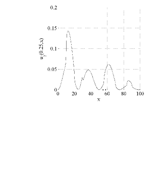
Figure 1: Example 1: a) exact habitat configuration $\mu$; b) measurement of $u_{\gamma}(0.25,x)$ which was used for recovering $\mu$; the domain $\omega$ is delimited by two black dots. The exact configuration $\mu$ was recovered after $1500$ iterations of the algorithm.

Example 2: the set $E$ is composed of step functions which can take 21 different values between $m$ and $M$.

The function $\mu\in E$ and the measurement $u_{\gamma}(\frac{t_{0}+t_{1}}{2},x)$ are depicted in Fig. 2, (a) and (b). Two elements of $E$ are said to be neighbours if they differ by $(M-m)/20$ on an interval of length $1$.

This time, the sequence ($\hat{\mu}_{n}$) stabilised on a configuration $\hat{\mu}$ (Fig. 2, (c)) after $7500$ iterations. The mean error in this case was $\frac{1}{100}\int_{0}^{100}|\mu(x)-\hat{\mu}(x)|dx=0.05.$

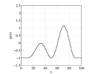
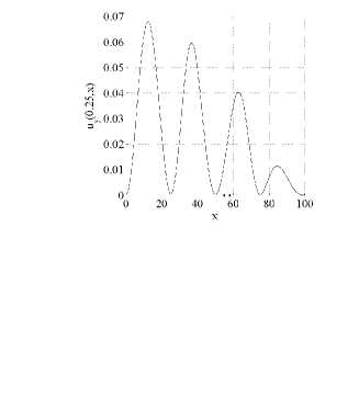
Figure 2: Example 2: a) exact habitat configuration $\mu$; b) measurement of $u_{\gamma}(0.25,x)$ which was used for recovering $\mu$; the domain $\omega$ is delimited by two black dots; c) configuration $\hat{\mu}:=\hat{\mu}_{7500}$, obtained after $7500$ iterations.

4.2 Two-dimensional case

Assume now that $\Omega=(0,20)\times(0,20)$, $\Omega_{1}=[2,18]\times[2,18]$, and that $\omega$ is the closed ball of centre $(7;7)$ and radius $3$ . Assume also that $M=2$ and $m=-1$, and that the initial data is $u_{i}=0.1xy/400\sin(x/4)^{2}\sin(y/4)^{2}$.

Example 3: $E$ is composed of binary functions which can only take the values $m$ and $M$ on each cell of a regular lattice.

We fixed $\mu\in E$ as in Fig. 3 (a). The measurement $u_{\gamma}(\frac{t_{0}+t_{1}}{2},x)$ is depicted in Fig. 3 (b). Two elements of $E$ are said to be neighbours if they differ only on one cell of the lattice.

The sequence ($\hat{\mu}_{n}$) stabilised on the exact configuration $\mu$ after 3000 iterations.

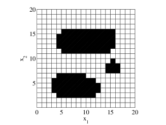
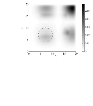
Figure 3: Example 3: a) exact habitat configuration $\mu$. In the black regions, the depicted function takes the value $2$; in the white regions, it takes the value $-1$. b) measurement of $u_{\gamma}(0.25,x)$ which was used for recovering $\mu$; the domain $\omega$ is delimited by a black circle. The exact configuration $\mu$ was recovered after $3000$ iterations.

Example 4: $E$ is composed of functions which can take $21$ different values between $m$ and $M$ on each cell of a regular lattice.

The configuration $\mu$ and the measurement $u_{\gamma}(\frac{t_{0}+t_{1}}{2},x)$ are depicted in Fig. 4 (a) and (b). Two elements of $E$ are said to be neighbours if they differ by $(M-m)/20$ on one cell of the lattice.

The sequence ($\hat{\mu}_{n}$) stabilised on a configuration $\hat{\mu}$ after 14000 iterations (Fig. 4, (c)). The mean error was $\frac{1}{20^{2}}\int_{0}^{20}\int_{0}^{20}|\mu(x,y)-\hat{\mu}(x,y)|dxdy=0.04.$

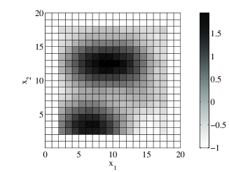
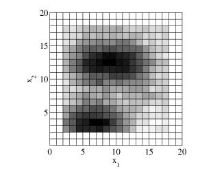
Figure 4: Example 4: a) exact habitat configuration $\mu$; b) measurement of $u_{\gamma}(0.25,x)$ which was used for recovering $\mu$; the domain $\omega$ is delimited by a black circle; c) approached configuration $\hat{\mu}_{14000}$. The darker the regions in (a), (b) and (c), the higher the values of the depicted functions.

5 Discussion and conclusion

We have shown that, for an invasive species whose density is well modelled by a reaction-diffusion equation, the spatial arrangement of the favourable and unfavourable regions can be measured indirectly through the population density at the beginning of the invasion. More precisely, we considered a logistic-like reaction-diffusion model, and we placed ourselves under the assumption that the initial population density was far from the environment carrying capacity (it can be reasonably assumed at the beginning of an invasion). In such a situation, the position of the favourable and unfavourable regions, modelled through the intrinsic growth rate coefficient $\mu$, may not be known a priori. This is especially true for exotic species whose hosts in native range and newly-colonised areas can be different. From our results, in the “ideal case” considered here, the position of these regions can be obtained through partial measurements of the population density. These partial measurements consist in two samples of the population density: 1) a “spatio-temporal” measurement, but very locally (in the small subset $\omega$) and during a short time period and, 2) a “spatial” measurement in the whole region susceptible to colonisation ($\Omega$).

The stochastic algorithm presented in section 3 shows explicitly how to reconstruct the habitat arrangement $\mu$ from the above partial measurements of the population density. This algorithm was proved to be effective in both one-dimensional and two-dimensional cases, in section 4, through several numerical experiments. In examples 1 and 3, the algorithm converged to the exact habitat configuration. In examples 2 and 4, the sizes of the sets of possible habitat configurations were increased compared to examples 1 and 3. In those cases, the algorithm converged to configurations which were close to the exact ones. It is noteworthy that the spatial measurement in $\Omega$ and the habitat arrangement $\mu$ can have very different shapes; therefore, $\mu$ cannot be straightforwardly deduced from this measurement.

These results can be helpful in preventing biological invasions. Indeed, a simple protocol, consisting of placing one trap in the invaded region, and recording the number of individuals captured by this trap over a short time-period (depending on the species characteristics), and performing a single survey of the number of individuals and their position in the whole considered region should allow, from our results, to detect the favourable areas, and to treat them preventively. As we have emphasised in Proposition 2.6.a, the knowledge of an estimate of the habitat arrangement $\mu$ also allows us to forecast the final population density, and therefore to detect the regions at higher risk, for instance in the case of harmful species. As recalled in Proposition 2.6.b, having a good estimate of the habitat arrangement $\mu$ is also crucial to forecast the fate of the invasive species: persistence or extinction.

On the other hand, we have to underline that our approach may not be adapted to some species, especially those which colonies are made of few individuals. Indeed, the diffusion operator of our model can be obtained as the macroscopic limit of uncorrelated random walks. With such an operator, by the parabolic maximum principle [16], it is known that, even with a compactly supported initial population density, the solution of our model is strictly positive everywhere on the domain as soon as $t>0$. This means that the solution, and therefore the information, propagate with infinite speed, which is not realistic for discrete populations. This could induce a practical limitation of our method to a certain type of species, which are well modelled by continuous diffusion processes even at low densities (typically some insect or plant species, with high carrying capacity and growth rate).

Note also that some of the mathematical tools used in this paper, and especially Carleman estimates (see Appendix A), were initially not adapted to the nonlinear model considered here. Thus, we first considered, in Theorem 2.2, the linear - or Malthusian - case. For populations whose density is far from the environment carrying capacity, the linear and the nonlinear problem have close solutions. In this situation, Theorem 2.4 extended the result of Theorem 2.2 to the nonlinear case of a logistic growth.

The results of this paper could be immediately extended to the case of spatially varying functions $\gamma(x)$. Another easy extension would be, for the “spatio-temporal” measurement, to use a partial boundary observation on a part $\Gamma^{+}$ of the domain boundary $\partial\Omega$ instead of sampling the population over a small domain $\omega$. Using a new Carleman estimate (see [21]) we are indeed able to write a stability result for the coefficient $\mu$, similar to that of Theorem 2.2, but with $\|\partial_{\mathbf{n}}(\partial_{t}u_{\gamma})-\partial_{\mathbf{n}}(\partial_{t}\tilde{v})\|^{2}_{L^{2}((t_{0},t_{1})\times\Gamma^{+})}$ instead of $\|\partial_{t}u_{\gamma}-\partial_{t}\tilde{v}\|^{2}_{L^{2}((t_{0},t_{1})\times\omega)}$ in the definition of the functional $G$.

6 Appendices

Let us introduce the following notations: for all $t,t^{\prime}\in\mathbb{R},$ with $t^{\prime}>t$, we denote $Q_{t}^{t^{\prime}}=(t,t^{\prime})\times\Omega$ and $\Sigma_{t}^{t^{\prime}}=(t,t^{\prime})\times\partial\Omega$. Throughout this section, with a slight abuse of notation, we designate by $C$ any upper bounds in our computations, provided they only depend on the parameters $\Omega,$ $\Omega_{1},$ $\omega,$ $\mathcal{B}_{\varepsilon},$ $D,$ $t_{0},$ $t_{1}$, $\underline{u_{i}}/\overline{u_{i}}$.

6.1 Appendix A: proof of Theorem 2.2

Carleman estimate

We recall here a Carleman-type estimate with a single observation. Let $\beta$ be a function in ${\cal C}^{2}(\overline{\Omega})$ such that

$$1<\beta<2\mbox{ in }\Omega,\ \ \beta=1\mbox{ on }\partial\Omega,\ \min\{|\nabla\beta(x)|,x\in\Omega\backslash\overline{\omega}\}>0\mbox{ and }{\partial}_{\bf n}\beta<0\mbox{ on }\partial\Omega,$$

where ${\bf n}$ denotes the outward unit normal to $\partial\Omega$. For $\lambda>0$ and $t\in(t_{0},t_{1})$, we define the following weight functions

$$\varphi(t,x)=\frac{e^{\lambda\beta(x)}}{(t-t_{0})(t_{1}-t)},\ \ \eta(t,x)=\frac{e^{2\lambda}-e^{\lambda\beta(x)}}{(t-t_{0})(t_{1}-t)}.$$

Let $q$ be a solution of the parabolic problem

$$\left\{\begin{array}[]{l}\partial_{t}q-D\Delta q+\alpha(x)q=f(t,x)\hbox{ in }Q_{t_{0}}^{t_{1}},\\ q=0\hbox{ on }\Sigma_{0}^{t_{1}},\\ q(0,x)=q_{0}(x)\hbox{ in }\Omega,\end{array}\right.\ (P)$$

for some functions $f\in L^{2}(Q_{t_{0}}^{t_{1}}),$ and $\alpha,q_{0}\in L^{\infty}(\Omega)$.

Then the following results are proved in [22]:

Lemma 6.1

Let $q$ be a solution of (P). Then, there exist three positive constants $\lambda_{0}$, $C_{0}$ and $s>1$, depending only on $\Omega$, $\omega$, $t_{0}$ and $t_{1}$ such that, for any $\lambda\geq\lambda_{0}$, the next inequalities hold:

$$\begin{array}[]{l}\hbox{a) }\|M_{1}(e^{-s\eta}q)\|^{2}_{L^{2}(Q_{t_{1}})}+\|M_{2}(e^{-s\eta}q)\|^{2}_{L^{2}(Q_{t_{1}})}+s\lambda^{2}\int_{Q_{t_{0}}^{t_{1}}}e^{-2s\eta}\varphi|\nabla q|^{2}\\ +s^{3}\lambda^{4}\int_{Q_{t_{0}}^{t_{1}}}e^{-2s\eta}\varphi^{3}q^{2}\leq C_{0}\left[s^{3}\lambda^{4}\int_{t_{0}}^{t_{1}}\int_{\omega}e^{-2s\eta}\varphi^{3}q^{2}+\int_{Q_{t_{0}}^{t_{1}}}e^{-2s\eta}\ (f-\alpha q)^{2}\right],\end{array}$$

where $M_{1}$ and $M_{2}$ are defined by $M_{1}\psi=-D\Delta\psi-s^{2}\lambda^{2}D|\nabla\beta|^{2}\varphi^{2}\psi+s(\partial_{t}{\eta})\psi$, and $M_{2}\psi=\partial_{t}\psi+2s\lambda D\varphi\nabla\beta.\nabla\psi+2s\lambda^{2}D\varphi|\nabla\beta|^{2}\psi.$ Moreover,

$$\begin{array}[]{l}\hbox{b) }s^{-2}\lambda^{-2}\int_{Q_{t_{0}}^{t_{1}}}e^{-2s\eta}\varphi^{-1}[(\partial_{t}q)^{2}+(\Delta q)^{2}]+\int_{Q_{t_{0}}^{t_{1}}}e^{-2s\eta}\varphi|\nabla q|^{2}+s^{2}\lambda^{2}\int_{Q_{t_{0}}^{t_{1}}}e^{-2s\eta}\varphi^{3}q^{2}\\ \leq C_{0}\left[s^{2}\lambda^{2}\int_{t_{0}}^{t_{1}}\int_{\omega}e^{-2s\eta}\varphi^{3}q^{2}+s^{-1}\lambda^{-2}\int_{Q_{t_{0}}^{t_{1}}}e^{-2s\eta}\ (f-\alpha q)^{2}\right].\end{array}$$

Stability estimate with one observation

Let $\mu,\tilde{\mu}\in\mathcal{M}$. We consider the solutions $v$ and $\widetilde{v}$ of the linear problems $(P_{\mu,0})$ and $(P_{\tilde{\mu},0}),$ respectively. We set $w=v-\widetilde{v}$, $y=\partial_{t}w$, and $\sigma=\mu-\widetilde{\mu}$. The function $y$ is a solution of:

$$\left\{\begin{array}[]{lll}{\partial}_{t}y=D\Delta y+\mu y+\sigma\partial_{t}\widetilde{v}&\mbox{in}&Q_{t_{0}}^{t_{1}},\\ y(t,x)=0&\mbox{on}&\Sigma_{t_{0}}^{t_{1}},\\ y(0,x)=\sigma u_{i}(x)&\mbox{in}&\Omega,\\ \end{array}\right.$$ (7)

The function $\eta(x,t)$ attains its minimum value with respect to the time at $t=T^{\prime}=\frac{t_{0}+t_{1}}{2}$. We set $\psi=e^{-s\eta}y$. Using the operator $M_{2}$, introduced in Lemma 6.1, we introduce, following [23] (see also [24] and [25]),

$$\mathcal{I}=\int_{t_{0}}^{T^{\prime}}\int_{\Omega}M_{2}\psi\;\psi.$$

Let $\lambda_{0}$ be fixed as in Theorem 6.1.

Lemma 6.2

Let $\lambda\geq\lambda_{0}$. There exists a constant $C$ such that

$$|\mathcal{I}|\leq C\left[s^{3/2}\lambda^{2}\int_{t_{0}}^{t_{1}}\int_{\omega}e^{-2s\eta}\varphi^{3}y^{2}+s^{-3/2}\lambda^{-2}\int_{Q_{t_{0}}^{t_{1}}}e^{-2s\eta}\sigma^{2}(\partial_{t}\widetilde{v})^{2}\right].$$ (8)

Proof: From the Hölder inequality, we have:

$$|\mathcal{I}|\leq s^{-3/2}\lambda^{-2}\left(\int_{0}^{T^{\prime}}\int_{\Omega}(M_{2}\psi)^{2}\right)^{1/2}\left(s^{3}\lambda^{4}\int_{0}^{T^{\prime}}\int_{\Omega}e^{-2s\eta}y^{2}\right)^{1/2}.$$

Thus using Young’s inequality, we obtain

$$|\mathcal{I}|\leq\frac{1}{4}s^{-3/2}\lambda^{-2}\left(\|M_{2}\psi\|_{L^{2}(Q_{t_{0}}^{t_{1}})}^{2}+s^{3}\lambda^{4}\int_{Q_{t_{0}}^{t_{1}}}e^{-2s\eta}\varphi^{3}y^{2}\right).$$ (9)

Applying inequality a) of Lemma 6.1 to $q:=y$, we obtain that there exists $C>0$, such that

$$\begin{array}[]{l}\|M_{2}\psi\|_{L^{2}(Q_{t_{0}}^{t_{1}})}^{2}+2s^{3}\lambda^{4}\int_{Q_{t_{0}}^{t_{1}}}e^{-2s\eta}\varphi^{3}y^{2}\\ \leq C\left[s^{3}\lambda^{4}\int_{t_{0}}^{t_{1}}\int_{\omega}e^{-2s\eta}\varphi^{3}y^{2}+\int_{Q_{t_{0}}^{t_{1}}}e^{-2s\eta}\ 2[\mu^{2}y^{2}+\sigma^{2}(\partial_{t}\widetilde{v})^{2}]\right].\end{array}$$ (10)

Furthermore, since $\mu$ is bounded, and since $\varphi$ is bounded from below by a positive constant, independent of $\lambda$, we get that

$$\int_{Q_{t_{0}}^{t_{1}}}2e^{-2s\eta}\mu^{2}y^{2}\leq s^{3}\lambda^{4}\int_{Q_{t_{0}}^{t_{1}}}e^{-2s\eta}\varphi^{3}y^{2},$$ (11)

for $\lambda$ large enough. Combining (10) and (11), we obtain:

$$\begin{array}[]{l}\|M_{2}\psi\|_{L^{2}(Q_{t_{0}}^{t_{1}})}^{2}+s^{3}\lambda^{4}\int_{Q_{t_{0}}^{t_{1}}}e^{-2s\eta}\varphi^{3}y^{2}\\ \leq C\left[s^{3}\lambda^{4}\int_{t_{0}}^{t_{1}}\int_{\omega}e^{-2s\eta}\varphi^{3}y^{2}+\int\int_{Q_{t_{0}}^{t_{1}}}e^{-2s\eta}\ \sigma^{2}(\partial_{t}\widetilde{v})^{2}\right].\end{array}$$ (12)

The conclusion of Lemma 6.2 follows from (9) and (12). $\Box$

Lemma 6.3

Let $\lambda\geq\lambda_{0}$. There exists a constant $C$ such that

$$\begin{array}[]{ll}\int_{\Omega}e^{{-2s\eta}(T^{\prime},x)}\ (\sigma\widetilde{v}(T^{\prime},x))^{2}&\leq C\left[s^{3/2}\lambda^{2}\int_{t_{0}}^{t_{1}}\int_{\omega}e^{-2s\eta}\varphi^{3}y^{2}\right.\\ &\left.+s^{-1}\lambda^{-2}\int_{Q_{t_{0}}^{t_{1}}}e^{-2s\eta(T^{\prime},x)}\sigma^{2}(\partial_{t}\widetilde{v})^{2}\right.\\ &\left.+\int_{\Omega}e^{{-2s\eta}(T^{\prime},x)}\ (D\Delta\ w(T^{\prime},x)+\mu w(T^{\prime},x))^{2}dx\right].\end{array}$$

Proof: Using integration by parts over $\Omega$ and the boundary condition $\psi=0$ on $\Sigma_{t_{0}}^{t_{1}}$, we get:

$$\begin{array}[]{ll}\mathcal{I}=&\frac{1}{2}\int_{Q_{t_{0}}^{T^{\prime}}}\partial_{t}(\psi^{2})\\ &-s\lambda D\int_{Q_{t_{0}}^{T^{\prime}}}\nabla\cdot({\varphi}\nabla\beta)\psi^{2}+2s\lambda^{2}D\int_{Q_{t_{0}}^{T^{\prime}}}{\varphi}|\nabla\beta|^{2}\psi^{2}.\end{array}$$ (13)

We then obtain

$$\frac{1}{2}\int_{\Omega}\psi\left(T^{\prime},\cdot\right)^{2}=\mathcal{I}-s\lambda^{2}D\int_{Q_{t_{0}}^{T^{\prime}}}{\varphi}|\nabla\beta|^{2}\psi^{2}dxdt+s\lambda D\int_{Q_{t_{0}}^{T^{\prime}}}{\varphi}\Delta\beta\psi^{2}\;dxdt$$

since $\psi(t_{0})=0$ and $\nabla\varphi=\lambda\varphi\nabla\beta$. As a consequence, for $\lambda>1$, and since $\Delta\beta$ is bounded in $\Omega$, we finally get

$$\int_{\Omega}e^{{-2s\eta}(T^{\prime},x)}y(T^{\prime},x)^{2}\;dx\leq 2|\mathcal{I}|+Cs\lambda^{2}\int_{t_{0}}^{T^{\prime}}\int_{\Omega}e^{{-2s\eta}}{\varphi}y^{2},$$ (14)

for some constant $C$. Using   $\varphi\leq\frac{(t_{1}-t_{0})^{2}}{4}\varphi^{3}$ and Lemma 6.1, we get that:

$$s\lambda^{2}\int_{Q_{t_{0}}^{T^{\prime}}}e^{{-2s\eta}}{\varphi}y^{2}\leq C\left[\lambda^{2}\int_{t_{0}}^{t_{1}}\int_{\omega}e^{-2s\eta}\varphi^{3}y^{2}+s^{-2}\lambda^{-2}\int_{Q_{t_{0}}^{t_{1}}}e^{-2s\eta}\ 2[\mu^{2}y^{2}+\sigma^{2}(\partial_{t}\widetilde{v})^{2}]\right].$$ (15)

Arguing as in the proof of Lemma 6.2 for equation (11), and since, for all $x\in\Omega$, the function $t\mapsto\eta(t,x)$ attains its minimum over $(t_{0},t_{1})$ at $t=T^{\prime}$, we finally obtain that, for $\lambda$ large enough, the last term in (14) is bounded from above by:

$$C\left[\lambda^{2}\int_{t_{0}}^{t_{1}}\int_{\omega}e^{-2s\eta}\varphi^{3}y^{2}+s^{-2}\lambda^{-2}\int_{Q_{t_{0}}^{t_{1}}}e^{-2s\eta(T^{\prime},x)}\sigma^{2}(\partial_{t}\widetilde{v})^{2}\right].$$

If we now observe that

$$y\left(T^{\prime},x\right)=D\Delta w\left(T^{\prime},x\right)+\mu w\left(T^{\prime},x\right)+\sigma\partial_{t}\widetilde{v}\left(T^{\prime},x\right),$$

we get:

$$\sigma^{2}\widetilde{v}\left(T^{\prime},x\right)^{2}\leq 2y\left(T^{\prime},x\right)^{2}+2\left[D\Delta w\left(T^{\prime},x\right)+\mu w\left(T^{\prime},x\right)\right]^{2},$$

and, since $s>1$, the estimate of lemma 6.3 follows. $\Box$

Lemma 6.4

We have $0\leq v,\tilde{v}\leq\overline{u_{i}}e^{Mt_{1}}$, and $|\partial_{t}\tilde{v}|\leq(D+M)\overline{u_{i}}e^{Mt_{1}}$ in $Q_{t_{0}}^{t_{1}}$.

Proof: From the parabolic maximum principle, we know that $v,\tilde{v}\geq 0$ in $Q_{t_{0}}^{t_{1}}$. Let $h$ be the solution of the ordinary differential equation

$$\left\{\begin{array}[]{l}h^{\prime}=hM\hbox{ on }\mathbb{R}_{+},\\ h(0)=\overline{u_{i}}.\end{array}\right.$$ (16)

The function $h$ is increasing and $H(t,\cdot):=h(t)$ is a supersolution of the equations satisfied by $v$ and $\tilde{v}$. As a consequence of the parabolic maximum principle, we have,

$$0\leq v,\tilde{v}\leq h(t_{1})=\overline{u_{i}}e^{Mt_{1}},\hbox{ in }Q_{t_{0}}^{t_{1}}.$$ (17)

Let us set $\rho:=\partial_{t}\tilde{v}$. The function $\rho$ satisfies:

$$\left\{\begin{array}[]{lll}{\partial}_{t}\rho=D\Delta\rho+\tilde{\mu}\rho&\mbox{in}&Q,\\ \rho(t,x)=0&\mbox{on}&\Sigma,\\ \rho(0,x)=D\Delta u_{i}(x)+\tilde{\mu}u_{i}&\mbox{in}&\Omega.\\ \end{array}\right.$$ (18)

Since $u_{i}\in\mathcal{D}$, $\rho(0,x)\in L^{\infty}(\Omega)$. Moreover, $H_{1}(t,x):=-(D+M)\overline{u_{i}}e^{Mt}$ and $H_{2}(t,x):=(D+M)\overline{u_{i}}e^{Mt}$ are respectively sub- and supersolutions of (18). The parabolic maximum principle leads to the inequalities,

$$-(D+M)\overline{u_{i}}e^{Mt_{1}}\leq\rho\leq(D+M)\overline{u_{i}}e^{Mt_{1}}\hbox{ in }Q_{t_{0}}^{t_{1}}.$$ (19)

$\Box$

From Lemmas 6.3 and 6.4, and since $\sigma$ vanishes outside $\Omega_{1}$, it follows that

$$\begin{array}[]{l}\int_{\Omega_{1}}e^{-2s\eta(T^{\prime},x)}\sigma^{2}\left(\widetilde{v}(x,T^{\prime})^{2}-Cs^{-1}\lambda^{-2}(D+M)^{2}\overline{u_{i}}^{2}e^{2Mt_{1}}\right)dx\leq\\[5.69054pt] Cs^{3/2}\lambda^{2}\int_{t_{0}}^{t_{1}}\int_{\omega}e^{-2s\eta}\varphi^{3}y^{2}+C\int_{\Omega}e^{{-2s\eta}(T^{\prime},x)}[(\Delta w(T^{\prime},x))^{2}+w(T^{\prime},x)^{2}]\;dx.\end{array}$$ (20)

Lemma 6.5

The ratio $\underline{u_{i}}/\overline{u_{i}}$ being fixed, there exists $r>0$, independent of $\tilde{\mu}$, $u_{i}$, $\underline{u_{i}}$ and $\overline{u_{i}}$, such that $\tilde{v}\left(T^{\prime},\cdot\right)>\overline{u_{i}}r$ in $\Omega_{1}$.

Proof: Let $\xi_{0}\leq 1$ be a smooth function in $\Omega$, such that $\xi_{0}\equiv 1$ in $\mathcal{B}_{\frac{\varepsilon}{2}}$ and $\xi_{0}\equiv 0$ in $\Omega\backslash\mathcal{B}_{\varepsilon}$. Let $\xi$ be the solution of

$$\left\{\begin{array}[]{l}\partial_{t}\xi=D\Delta\xi-M\xi\hbox{ in }Q,\\ \xi(t,x)=0\hbox{ on }\Sigma,\\ \xi(0,x)=(\underline{u_{i}}/\overline{u_{i}})\xi_{0}(x)\hbox{ in }\Omega.\end{array}\right.$$ (21)

Let us set $r:=\displaystyle{\inf_{x\in\Omega_{1}}\xi\left(T^{\prime},x\right)}$. From the strong parabolic maximum principle, $\xi>0$ in $Q_{t_{0}}^{t_{1}}$, and therefore, we get that $r>0$, since $\Omega_{1}$ is a closed subset of $\Omega$. Moreover, the parabolic maximum principle also yields $\overline{u_{i}}\xi\leq\tilde{v}$ in $Q_{t_{0}}^{t_{1}}$. In particular, we get $\tilde{v}\left(T^{\prime},x\right)\geq\overline{u_{i}}r>0$ in $\Omega_{1}$. $\Box$

From Lemma 6.5, it follows that, for $\displaystyle{\lambda\geq\sqrt{\frac{2C}{s}}\frac{(D+M)e^{Mt_{1}}}{r}}$, the term $\widetilde{v}(x,T^{\prime})^{2}-Cs^{-1}\lambda^{-2}(D+M)^{2}\overline{u_{i}}^{2}e^{2Mt_{1}}$ in (20) satisfies:

$$\widetilde{v}(x,T^{\prime})^{2}-Cs^{-1}\lambda^{-2}(D+M)^{2}\overline{u_{i}}^{2}e^{2Mt_{1}}\geq\overline{u_{i}}^{2}\frac{r^{2}}{2}>0\hbox{ in }\Omega_{1}.$$

We deduce that, for $\lambda$ large enough,

$$\begin{array}[]{l}\int_{\Omega_{1}}e^{-2s\eta(T^{\prime},x)}\sigma^{2}dx\\ \leq\frac{C}{\overline{u_{i}}^{2}}\left(s^{3/2}\lambda^{2}\int_{t_{0}}^{t_{1}}\int_{\omega}e^{-2s\eta}\varphi^{3}y^{2}+\int_{\Omega}e^{{-2s\eta}(T^{\prime},x)}((\Delta w(T^{\prime},x))^{2}+w(T^{\prime},x)^{2})dx\right).\end{array}$$ (22)

Using the fact that $e^{-2s\eta}\varphi^{3}$ remains bounded in $Q_{t_{0}}^{t_{1}}$, we finally obtain

$$\|\sigma\|^{2}_{L^{2}(\Omega_{1})}\leq\frac{C}{\overline{u_{i}}^{2}}\left(\int_{t_{0}}^{t_{1}}\int_{\omega}y^{2}+\int_{\Omega}((\Delta w(T^{\prime},x))^{2}+w(T^{\prime},x)^{2})\;dx\right).$$ (23)

Recalling that $w=v-\widetilde{v}$, $y=\partial_{t}(v-\widetilde{v})$, (23) implies the result of Theorem 2.2.

6.2 Appendix B: Proof of Theorem 2.4

Let $u_{\gamma}$ be the solution of $(P_{\mu,\gamma})$, and let $v$ be the solution of $(P_{\mu,0})$. Let us set $z_{\gamma}:=v-u_{\gamma}$. The function $z_{\gamma}$ is a solution of

$$\left\{\begin{array}[]{l}\partial_{t}z_{\gamma}-D\Delta z_{\gamma}=z_{\gamma}\mu(x)+\gamma u_{\gamma}^{2}\hbox{ in }Q,\\ z_{\gamma}(t,x)=0\hbox{ on }\Sigma,\\ z_{\gamma}(0,x)=0\hbox{ in }\Omega.\end{array}\right.$$ (24)

It follows from the parabolic maximum principle that $z_{\gamma}(t,x)>0$ in $Q_{t_{0}}^{t_{1}}$. Thus $u_{\gamma}\leq v$ in $Q_{t_{0}}^{t_{1}}$. Using the result of Lemma 6.4, we thus obtain:

$$u_{\gamma}(t,x)\leq\overline{u_{i}}e^{Mt_{1}}\hbox{ in }Q_{t_{0}}^{t_{1}}.$$ (25)

Let $k$ be the solution of

$$\left\{\begin{array}[]{l}k^{\prime}=kM+\gamma\overline{u_{i}}^{2}e^{2Mt_{1}}\hbox{ on }\mathbb{R}_{+},\\ k(0)=0.\end{array}\right.$$ (26)

Since $K(t,x):=k(t)$ is a supersolution of (24), we obtain that $z_{\gamma}(t,x)\leq k(t)$ in $Q_{0}^{t_{1}}$. Thus, since $k$ is increasing,

$$z_{\gamma}(t)\leq k(t_{1})=\frac{\gamma\overline{u_{i}}^{2}e^{2Mt_{1}}}{M}(e^{Mt_{1}}-1)\hbox{ in }Q_{t_{0}}^{t_{1}}.$$ (27)

Standard parabolic estimates (see e.g. [16]) then imply, using (17), (25), (27) and the hypothesis $\|u_{i}\|_{C^{2}(\overline{\Omega})}\leq\overline{u_{i}}$, that:

$$\|\partial_{t}v\|_{L^{2}(Q_{t_{0}}^{t_{1}})} = \mathcal{O}(\|\mu v\|_{L^{2}(Q_{0}^{t_{1}})}+\|u_{i}\|_{H^{1}_{0}(\Omega)})=\mathcal{O}(\overline{u_{i}}),$$ (28)

$$\|\partial_{t}z_{\gamma}\|_{L^{2}(Q_{t_{0}}^{t_{1}})} = \mathcal{O}(\|z_{\gamma}\mu+\gamma u_{\gamma}^{2}\|_{L^{2}(Q_{0}^{t_{1}})})=\mathcal{O}(\overline{u_{i}}^{2}),$$ (29)

$$\|\partial_{t}u_{\gamma}\|_{L^{2}(Q_{t_{0}}^{t_{1}})} = \mathcal{O}(\|u_{\gamma}(\mu-\gamma u_{\gamma})\|_{L^{2}(Q_{0}^{t_{1}})}+\|u_{i}\|_{H^{1}_{0}(\Omega)})$$ (30)

$$= \mathcal{O}(\overline{u_{i}}),$$

$$\sup_{t_{0}\leq t\leq t_{1}}\|v(t,.)\|_{H^{2}(\Omega)} = \mathcal{O}(\|\mu v\|_{H^{1}(0,t_{1};L^{2}(\Omega))}+\|u_{i}\|_{H^{2}(\Omega)})=\mathcal{O}(\overline{u_{i}})$$ (31)

$$\sup_{t_{0}\leq t\leq t_{1}}\|z_{\gamma}(t,.)\|_{H^{2}(\Omega)} = \mathcal{O}(\|z_{\gamma}\mu+\gamma u_{\gamma}^{2}\|_{H^{1}(0,t_{1};L^{2}(\Omega))}),$$ (32)

$$= \mathcal{O}(\overline{u_{i}}^{2}).$$

Using (29) and (32), we get:

$$G_{\mu}(\gamma,\mu)=\mathcal{O}(\overline{u_{i}}^{4}).$$ (33)

Moreover, since $u_{0}=v$, we have

$$\begin{array}[]{rl}G_{\mu}(\gamma,\tilde{\mu})&=G_{\mu}(0,\tilde{\mu})+G_{\mu}(\gamma,\mu)+2\langle\partial_{t}z_{\gamma},\partial_{t}v-\partial_{t}\tilde{v}\rangle_{L^{2}(Q_{t_{0}}^{t_{1}})}\\ &+2\langle\Delta z_{\gamma}\left(T^{\prime},\cdot\right),\Delta v\left(T^{\prime},\cdot\right)-\Delta\tilde{v}\left(T^{\prime},\cdot\right)\rangle_{L^{2}(\Omega)}\\ &+2\langle z_{\gamma}\left(T^{\prime},\cdot\right),v\left(T^{\prime},\cdot\right)-\tilde{v}\left(T^{\prime},\cdot\right)\rangle_{L^{2}(\Omega)}.\end{array}$$ (34)

Thus, using (28) and (31), which are true for both $v$ and $\tilde{v}$, and (29), (32), (33), together with Cauchy-Schwarz inequality, we get:

$$|G_{\mu}(\gamma,\tilde{\mu})-G_{\mu}(0,\tilde{\mu})|=\mathcal{O}(\overline{u_{i}}^{3}).$$ (35)

$\Box$

6.3 Appendix C: Definitions of the state spaces $E$ and of their neighbourhood systems.

In examples $1$ and $2$ of section $4$, $E$ is defined by

$$E:=\left\{\rho\in\mathcal{M},\ \rho(x)=\sum_{k=10}^{89}\alpha_{k}\chi_{k}(x)\hbox{ in }\Omega_{1},\hbox{ and }\rho(x)=m\hbox{ in }\Omega\backslash\Omega_{1}\right\},$$

where $\chi_{k}$ are the characteristic functions of the intervals $(\frac{k}{100},\frac{k+1}{100})$, and $\alpha_{k}$ are real numbers taken in finite subsets of $[m,M]$.

In example $1$, $\alpha_{k}\in\{-1,2\}$, and two distinct elements $\nu_{1}$, $\nu_{2}$ of $E$, with $\nu_{1}=\sum_{k=10}^{89}\alpha_{1,k}\chi_{k}(x)$ and $\nu_{2}=\sum_{k=10}^{89}\alpha_{2,k}\chi_{k}(x)$ in $\Omega_{1}$, are defined as neighbours if and only if there exists a unique integer $k_{0}$ in $[10,89]$ such that $\alpha_{1,k_{0}}\neq\alpha_{2,k_{0}}$. Note that, in this case, the number of elements in $E$ is $2^{80}$.

In example $2$, $\alpha_{k}\in\{(M-m)j/20+m,\hbox{ for }j=0\ldots 20.$}, and the neighbourhood system is defined as follows: two distinct elements $\nu_{1}$, $\nu_{2}$ of $E$, with $\nu_{1}=\sum_{k=10}^{89}\alpha_{1,k}\chi_{k}(x)$ and $\nu_{2}=\sum_{k=10}^{89}\alpha_{2,k}\chi_{k}(x)$ in $\Omega_{1}$, are neighbours if and only if (i) there exists a unique integer $k_{0}$ in $[10,89]$ such that $\alpha_{1,k_{0}}\neq\alpha_{2,k_{0}}$, (ii) additionally, $|\alpha_{1,k_{0}}-\alpha_{2,k_{0}}|=(M-m)/20$. Note that, in such a situation, the number of elements in $E$ is $21^{80}$.

In examples $3$ and $4$ of section $4$, $E$ is defined by

$$E:=\left\{\rho\in\mathcal{M},\ \rho(x)=\sum_{i,j=2}^{17}\alpha_{i,j}\chi_{i,j}(x)\hbox{ in }\Omega_{1},\hbox{ and }\rho(x)=m\hbox{ in }\Omega\backslash\Omega_{1}\right\},$$

where $\chi_{i,j}$ are the characteristic functions of the square cells $(i/20,i/20+1/20)\times(j/20,j/20+1/20)$, and $\alpha_{i,j}$ are real numbers taken in finite subsets of $[m,M]$.

In example $3$, $\alpha_{i,j}\in\{-1,2\}$. In this case, the number of elements in $E$ is $2^{256}$. Two distinct elements $\nu_{1}$, $\nu_{2}$ of $E$, with $\nu_{1}=\sum_{i,j=2}^{17}\alpha^{1}_{i,j}\chi_{i,j}(x)$ and $\nu_{2}=\sum_{i,j=2}^{17}\alpha^{2}_{i,j}\chi_{i,j}(x)$ for $x\in\Omega_{1}$, are defined as neighbours if and only if there exists a unique couple $(i_{0},j_{0})$ of integers comprised between $2$ and $17$ such that $\alpha^{1}_{i_{0},j_{0}}\neq\alpha^{2}_{i_{0},j_{0}}$.

In example $4$ $\alpha_{i,j}\in\{(M-m)j/20+m,\hbox{ for }j=0\ldots 20.$}. The number of elements in $E$ is ${21}^{256}$. In this case, two distinct elements $\nu_{1}$, $\nu_{2}$ of $E$, with $\nu_{1}=\sum_{i,j=2}^{17}\alpha^{1}_{i,j}\chi_{i,j}(x)$ and $\nu_{2}=\sum_{i,j=2}^{17}\alpha^{2}_{i,j}\chi_{i,j}(x)$ for $x\in\Omega_{1}$, are defined as neighbours if and only if (i) it exists a unique couple $(i_{0},j_{0})$ of integers comprised between $2$ and $17$ such that $\alpha^{1}_{i_{0},j_{0}}\neq\alpha^{2}_{i_{0},j_{0}}$; and (ii) additionally $|\alpha^{1}_{i_{0},j_{0}}-\alpha^{2}_{i_{0},j_{0}}|=(M-m)/20$.

References

- [1] A.M. Liebhold, W.L. MacDonald, D. Bergdahl, V.C. Mastro, Invasion by exotic forest pests: A threat to forest ecosystems, Forest Sciences Monographs 30 (1995) 1.
- [2] National Invasive Species Information Center, USDA 2006, Executive Order 13112.
- [3] J.G. Skellam, Random dispersal in theoretical populations, Biometrika 38 (1951) 196.
- [4] N. Shigesada, K. Kawasaki, Biological Invasions: Theory and Practice, Oxford Series in Ecology and Evolution, Oxford University Press, Oxford, 1997.
- [5] P. Turchin, Quantitative Analysis of Movement: Measuring and Modeling Population Redistribution in Animals and Plants, Sinauer Associates, Sunderland, MA, 1998.
- [6] A. Okubo, S.A. Levin, Diffusion and Ecological Problems - Modern Perspectives, Second edition, Springer-Verlag, 2002.
- [7] R.A. Fisher, The wave of advance of advantageous genes, Ann. Eugenics 7 (1937) 355.
- [8] A.N. Kolmogorov, I.G. Petrovsky, N.S. Piskunov, Étude de l’équation de la diffusion avec croissance de la quantité de matière et son application à un problème biologique, Bull. Univ. État Moscou, Série Internationale A 1 (1937) 1.
- [9] H. Berestycki, F. Hamel, L. Roques, Analysis of the periodically fragmented environment model : I - Species persistence, J. Math. Biol. 51 (1) (2005) 75.
- [10] H. Berestycki, F. Hamel, L. Roques, Analysis of the periodically fragmented environment model : II - Biological invasions and pulsating travelling fronts, J. Math. Pures Appl. 84 (8) (2005) 1101.
- [11] N. Kinezaki, K. Kawasaki, N. Shigesada, Spatial dynamics of invasion in sinusoidally varying environments Popul. Ecol. 48 (2006) 263.
- [12] N. Shigesada, K. Kawasaki, E. Teramoto, Traveling periodic waves in heterogeneous environments, Theor. Popul. Biol. 30 (1986) 143.
- [13] R.S. Cantrell, C. Cosner, Spatial Ecology via Reaction-Diffusion Equations, Series In Mathematical and Computational Biology, John Wiley and Sons, Chichester, Sussex UK, 2003.
- [14] L. Roques, R.S. Stoica, Species persistence decreases with habitat fragmentation: an analysis in periodic stochastic environments, J. Math. Biol. 55 (2007) 189.
- [15] L. Roques, M.D. Chekroun, On population resilience to external perturbations. SIAM J. Appl. Math. 68 (1) (2007) 133.
- [16] L.C. Evans, Partial Differential Equations, University of California, Berkeley - AMS, 1998.
- [17] L. Roques, F. Hamel, Mathematical analysis of the optimal habitat configurations for species persistence, Mathematical Biosciences 210 (2007) 34.
- [18] B. Hajek, Cooling schedules for optimal annealing, Math. Oper. Res. 13 (1988) 311.
- [19] D. Henderson, S.H. Jacobson, A.W. Johnson, 2003, The Theory and Practice of Simulated Annealing, Handbook on Metaheuristics, in: F. Glover, G. Kochenberger (Eds.), Kluwer Academic Publishers, Norwell MA, 2003, p. 287.
- [20] S. Kirkpatrick, C.D. Gelatt, M.P. Vecchi, Optimization by Simulated Annealing, Science 220 (1983) 671.
- [21] P. Albano, D. Tataru, Carleman estimates and boundary observability for a coupled parabolic-hyperbolic system, Electron. J. Differential Equations 22 (2000) 1.
- [22] A. Fursikov, Optimal control of distribued systems, Translations of Mathematical Monographs, American Mathematical Society, Providence, RI, 2000.
- [23] L. Baudouin, J.P. Puel, Uniqueness and stability in an inverse problem for the Schrödinger equation, Inverse Problems 18 (2002) 1537.
- [24] M. Cristofol, P. Gaitan, H. Ramoul, Inverse problems for a two by two reaction-diffusion system using a Carleman estimate with one observation, Inverse Problems 22 (2006) 1561.
- [25] L. Cardoulis, M. Cristofol, P. Gaitan, Inverse problem for a Schrödinger operator in an unbounded strip, J. Inverse Ill-Posed Problems V (16) (2008) 127.