Pion Polarizability in the NJL model and Possibilities of its Experimental Studies in Coulomb Nuclear Scattering

Abstract

The charge pion polarizability is calculated in the Nambu-Jona-Lasinio model, where the quark loops (in the mean field approximation) and the meson loops (in the $1/N_{c}$ approximation) are taken into account. We show that quark loop contribution dominates, because the meson loops strongly conceal each other. The sigma-pole contribution $(m^{2}_{\sigma}-t)^{-1}$ plays the main role and contains strong t-dependence of the effective pion polarizability at the region $|t|\geq 4M_{\pi}^{2}$. Possibilities of experimental test of this sigma-pole effect in the reaction of Coulomb Nuclear Scattering are estimated for the COMPASS experiment.

1. Introduction

Elementary particle polarizabilities $\alpha^{E},~{}\alpha^{H}$ were introduced as coefficients of low energy expansion of the Compton effect amplitude [1] using the definition of the effective potential energy:

$$V_{\rm eff}=-\frac{1}{2}[\alpha^{E}E^{2}+\alpha^{H}H^{2}]\Big{|}_{\alpha^{E}=-\alpha^{H}}=\frac{\alpha^{E}}{4}F^{2}_{\mu\nu}.$$ (1)

These coefficients as well as the electromagnetic radius are constants characterizing the internal structure of particles.

The values of charged pion polarizabilities $\alpha^{H},\alpha^{\rm E}_{\pi}$ was measured in Serpukhov [2]

$$\alpha_{\pi}^{E}\simeq-\alpha^{\rm H}_{\pi}=(6.8\pm 1.8)\cdot 10^{-4}{\mbox{\rm fm}}^{3}$$ (2)

and MAMI [3]

$$\alpha_{\pi}^{E}\simeq-\alpha^{\rm H}_{\pi}=(5.8\pm 1.7)\cdot 10^{-4}{\mbox{\rm fm}}^{3}$$ (3)

and was extracted from the MARK II data [4] in [5]

$$\alpha_{\pi}^{E}\simeq-\alpha^{\rm H}_{\pi}=(2.2\pm 1.6)\cdot 10^{-4}{\mbox{\rm fm}}^{3}.$$ (4)

One can see that the precision of the experimental measurements is too low to distinguish between the many predictions of the value of the charged pion polarizability obtained in various quark, chiral, dispersion and other models (see e.g. the reviews [6, 7, 8, 9, 10]).

There is a hope that new more precise measurements of the pion polarizabilities at the COMPASS experiment at CERN [11, 12, 13, 14] provide a good opportunity for the verification of these models.

The idea to investigate the charged pion polarizability in radiative $\pi^{-}$ meson scattering in the nuclear Coulomb field was proposed in [15]. It was shown in [15] that in the reaction

$$\pi^{-}+(A,Z)=\pi^{-}+(A,Z)+\gamma,$$ (5)

the Coulomb amplitude dominates for very small four-momentum transfers $\left|t\right|\leq 2\times 10^{-4}\left(~{}\mbox{GeV}/c\right)^{2}$ and the contribution from the pion polarizability to the Compton effect increases with the decrease of the Coulomb transfer.

The first experiment proposed in [15] was fulfilled at SIGMA-AYAKS spectrometer [2] in the context of the first predictions of the pion polarizability value in the quantum field theory approach [6, 17] to the non-polynomial Effective Chiral Lagrangian [18]. The results of calculation in [16] can be presented as the sum of both the fermion loops and the meson ones

$${\alpha^{E}_{\pi^{\pm}}}(t) = {\left(\alpha_{\pi^{\pm}}\right)_{ch}}\left[{\beta^{\rm fermion}_{\pi^{\pm}}}(t)+{\beta^{\rm pion}_{\pi^{\pm}}}(t)\right],$$ (6)

where $t$ is given in the experimental region $|t/(2M_{\pi})^{2}|\sim 1$ [2] and

$${\left(\alpha_{\pi^{\pm}}\right)_{ch}}=\dfrac{\alpha}{2\pi F^{2}_{\pi}m_{\pi}}=5.8\times 10^{-4}fm{}^{-3};$$ (7)

is the chiral limit, here $F_{\pi}=93$ MeV and $\alpha=\dfrac{e^{2}}{4\pi}=\dfrac{1}{137}$. The baryon loops gave the main contribution ${\beta^{\rm fermion}}_{\pi^{\pm}}\simeq 1$, whereas the meson loop contribution was small and negative ${\beta^{\rm pion}}_{\pi^{\pm}}\simeq-0.1$. It disagrees with the value ${\beta^{\rm pion}}_{\pi^{\pm}}\simeq+0.5$ obtained in [19] in the Chiral Perturbation Theory [20]. The authors of [19] associated this value ${\beta^{\rm pion}}_{\pi^{\pm}}\simeq+0.5$ with additional Chiral Lagrangians at order $p^{4}$. These low energy Lagrangians can contain the hadron contributions including the fermion loop one in the hidden form.

The problem of the ambiguities of the pion polarizability obtained from the Effective Chiral Lagrangians can be clear up by both the direct experimental measurements and the results obtained on the fundamental level of the QCD motivated quark models.

The calculations of the pion polarizability in the quark NJL model [8, 21, 22] motivated by QCD [23, 24] were fulfilled in [8, 25] in the framework of the mean field approximation, where the quark loops only are taken into account and the result ${\beta^{\rm quark}}^{\rm NJL}_{\pi^{\pm}}\simeq 1$ was obtained in agreement with the quark-baryon duality [26].

In this paper, we take into account also the meson loops. They appear in the next over $(1/N_{c})$ approximation. The NJL model results on the charge pion polarizability are summed and compared with other theoretical models.

The possibilities of the experimental tests of the NJL model predictions in reaction of Coulomb Nuclear Scattering will be estimated for the COMPASS experiment.

The content of the paper is the following. In Section 2., the kinematics of experiments [2] was chosen to detect with good efficiency the Compton effect events on pion with photon energies in the range $70-900~{}\mbox{MeV}$ in the pion rest frame. The pion polarizability is calculated in Section 3. Section 4 is devoted to discussion of possibility of the experimental test of the prediction of NJL model at COMPASS.

2. Kinematics of Pion Compton Effect

We consider the process: $\pi^{-}+(A,Z)=\pi^{-}+(A,Z)+\gamma$

$$\pi[p_{1}]~{}~{}+~{}~{}\gamma^{*}[q_{1}]~{}~{}\to~{}~{}\pi[p_{2}]~{}~{}+~{}~{}\gamma[q_{2}],$$ (8)

where the components of 4-vectors $[p_{1},q_{1},p_{2},q_{2}]$ are chosen in the form

$$p_{1}=\left(\varepsilon,~{}~{}~{}~{}~{}~{}~{}~{}~{}~{}~{}~{}~{}\varepsilon-\frac{M^{2}_{\pi}}{2\varepsilon},~{}~{}~{}~{}~{}~{}~{}~{}~{}~{}~{}~{}~{}~{}~{}~{}~{}~{}~{}0,~{}~{}~{}~{}0\right)$$ (9)

$$q_{1}=\left(\frac{Q^{2}}{2M_{\rm Nuc}},~{}~{}~{}~{}~{}{Q}=-\frac{M^{2}_{\pi}\omega^{2}+p_{t}^{2}}{2\omega(1-\omega)\varepsilon},~{}~{}~{}~{}~{}~{}0,~{}~{}~{}~{}0\right)$$ (10)

$$p_{2}=\left((1-\omega)\varepsilon,~{}~{}(1-\omega)\varepsilon-\frac{M^{2}_{\pi}+p_{t}^{2}}{2(1-\omega)\varepsilon},~{}~{}~{}p_{t},~{}~{}~{}~{}0\right)$$ (11)

$$q_{2}=\left(\varepsilon\omega,~{}~{}~{}~{}~{}~{}~{}~{}~{}~{}~{}\varepsilon\omega-\frac{p_{t}^{2}}{2\omega\varepsilon},~{}~{}~{}~{}~{}~{}~{}~{}~{}~{}~{}~{}~{}-p_{t},~{}~{}~{}~{}0\right).$$ (12)

where $\varepsilon$ is the energy of incoming pion, $M_{\rm Nuc}$ is the mass of the nuclear target and $\omega$ is the relative energy of emitted photon.

$$Q=-\frac{\omega^{2}M_{\pi}^{2}+p^{2}_{t}}{2\varepsilon\omega(1-\omega)}\equiv\frac{t}{2\varepsilon\omega},~{}~{}~{}~{}~{}~{}~{}~{}$$ (13)

is four-momentum transfer, and

$$t=(p_{1}-p_{2})^{2}=-\frac{M_{\pi}^{2}\omega^{2}+p^{2}_{t}}{(1-\omega)}$$ (14)

is one of Mandelstamm variables.

Amplitude is

$$A=A_{c}e^{i\phi}+A_{s},$$

where

$$A_{c}=(4\pi)^{3/2}e^{3}\frac{4M_{N}Z\varepsilon^{\mu}}{Q^{2}}\left\{g_{0\mu}-\frac{\varepsilon p_{2\mu}}{(p_{2}q_{2})}+\frac{(1-\varepsilon)p_{1\mu}}{(p_{1}q_{2})}+\beta[g_{0\mu}(q_{2}q_{1})-\varepsilon\omega q_{1\mu}]\right\}$$

is the Coulomb amplitude; $A_{s}=(4\pi)^{3/2}e^{2}M_{N}\varepsilon^{\mu}T_{\mu}$ is amplitude of the nuclear scattering; $\phi$ is the phase of the Coulomb - nuclear scattering; Z is the charge of a nucleus; $M_{N}$ is the mass of a nucleus; $\varepsilon^{\mu}$ is the vector of the polarization of a photon; $g_{\mu\nu}={\rm diag(1,-1,-1,-1)}$; $\alpha_{\pi}=\alpha\beta_{-}/M_{\pi}$ is the polarizability of a pion $\pi^{-}$; $T_{\mu}$ is the amplitude of a nuclear radiation scattering.

3. Polarizability of a pion in NJL model

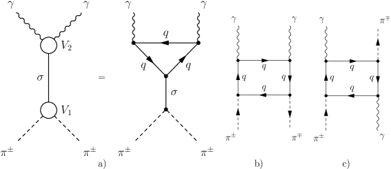
Figure 1:

3.1. Mean field approximation

The calculations of the pion polarizability in the NJL model [8, 21, 22] were fulfilled in [8, 25] in the approximation. It was shown in [8, 25] that in this mean field approximation the main contribution goes from the the quark loops given in Figs. 1a,b,c. The first diagram in Fig. 1a contains two vertexes

$$V_{1}=\dfrac{4m_{u}^{2}}{F_{\pi}}\sqrt{Z},~{}~{}V_{2}=\dfrac{10\alpha}{9\pi F_{\pi}\sqrt{Z}}\overline{F}(t_{u})[g_{\mu\nu}q_{1}\cdot q_{2}-{q_{1}}_{\mu}{q_{2}}_{\nu}]\varepsilon_{\mu}(q_{1})\varepsilon_{\nu}(q_{2})$$ (18)

and the sigma meson propagator $1/(m_{\sigma}^{2}-t)$, where $m_{u}=280$ MeV is the constituent mass of the u-(d-) quarks and $t_{u}=t/(4m_{u}^{2})<0$ is given in the region of negative values, the factor $Z$ has a form $Z=\left(1-\frac{6m_{u}^{2}}{M_{A_{1}}^{2}}\right)^{-1}$; here $M_{A_{1}}=1260MeV$ is the mass of $A_{1}$-meson [27].

The t-dependence of the radiative triangle and box diagrams is very weak and it can be neglected. In particular, the triangle diagram formfactor in the region of measurement $|t_{u}|\sim 1/4$ can be identified with the unit 1

$$\overline{F}(t_{u}) = 3\int\limits_{0}^{1}dx\int\limits_{0}^{1}dyy\frac{1-4y^{2}x(1-x)}{1-4y^{2}x(1-x)t_{u}}=1+t_{u}\frac{7}{90}...$$ (19)

within order of 2% accuracy.

Taking into account the contribution of the diagrams in Figs. 1b,c in the lowest $q_{1}\cdot q_{2}$ approximation

$$\frac{\alpha}{\pi F_{\pi}}[g_{\mu\nu}q_{1}\cdot q_{2}-{q_{1}}_{\mu}{q_{2}}_{\nu}]\varepsilon_{\mu}(q_{1})\varepsilon_{\nu}(q_{2})$$ (21)

one can obtain the next expression for polarizability [25]

$${\alpha^{E}_{\pi^{\pm}}}(t)=\dfrac{\alpha}{18\pi F^{2}_{\pi}m_{\pi}}\left[\frac{40m^{2}_{u}}{m_{\sigma}^{2}-t}-{1}\right]={\left(\alpha_{\pi^{\pm}}\right)_{ch}}{\beta^{\rm quark}_{\pi^{\pm}}}(t),$$ (22)

where the $t$-dependence of the quark loops is neglected.

Using the definitions (6) and (7) and the NJL relation [8]

$$m^{2}_{\sigma}=4m_{u}^{2}+M^{2}_{\pi},$$ (23)

one can obtain the final result in the form

$$\beta^{\rm quark}_{\pi^{\pm}}(t)=\frac{10}{9}\frac{4m^{2}_{u}}{m_{\sigma}^{2}-t}-\frac{1}{9}$$ (24)

where the chiral limit ($t=0$, $M_{\pi}^{2}=0$ and $m^{2}_{\sigma}=4m_{u}^{2}$) corresponds to unit $\beta^{\rm quark}_{\pi^{\pm}}(0)\to 1$.

3.2. Meson loops

Figure 2:

Figure 3:

Figure 4:

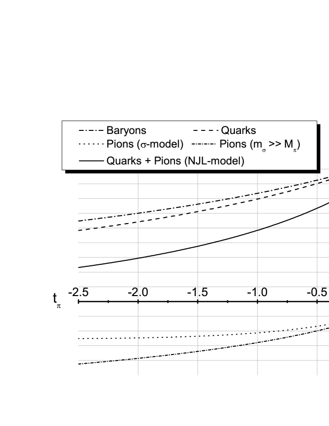
Figure 5: These are the pion polarizability contributions (ordinate axis) taken separately and their sum (quarks + mesons) given by Eq. (28) in terms of $t_{\pi}=t/(2M_{\pi})^{2}$ (abscissa).

As it was shown in [29] in two-photon decays of scalar mesons besides the quark loops contribution in the mean field approximation the important role is played by meson loops in the next $1/N_{c}$ order approximation. In particular, in two-photon decays of $f_{0}(980)$ meson, the meson loops plays the dominant role [29, 30]. The comparably large values of the meson loop contributions in comparison with the quark loops caused by the fractional electric charge of quarks, while the mesons have an integer charges. Therefore, in description of radiative decays of scalar meson both the quark and meson loops are necessary to take them into account. In papers [29] it was shown that this approach leads to satisfactory agreement with the recent experimental data on two-photon decays of scalar mesons $\sigma(600)$, $f_{0}(980)$ and $a_{0}(980)$.

Therefore, in description of pion polarizability in the electromagnetic vertex $\sigma\to 2\gamma$ the quark triangle loop should be supplied by meson loop contributions.

However, in the case of the Compton effect, there is a set of diagrams with internal sigma meson line. These diagrams also give the noticeable contribution to polarizability and have an opposite sign in comparison with the meson diagrams on Fig. 4.

As a result the contributions of the meson loops in Figs. 2,3 strongly conceal the ones of meson loops in Fig. 4.

Finally the pion loop contributions take the form

$$\beta^{\rm pion}_{\pi^{\pm}}(t)=\frac{m_{u}^{2}}{M_{\pi}^{2}}\left[\frac{4m_{u}^{2}}{m^{2}_{\sigma}-t}-1\right]\frac{\Phi(t_{\pi})}{3}=\frac{m^{2}_{\sigma}-M_{\pi}^{2}}{m^{2}_{\sigma}-t}\left(t_{\pi}-\frac{1}{4}\right)\frac{\Phi(t_{\pi})}{3},$$ (25)

where in this model $m^{2}_{\sigma}=4m_{u}^{2}+M_{\pi}^{2}$ and ${\Phi}(t_{\pi})$ is the function of $t_{\pi}=t/(2M_{\pi})^{2}=q_{1}q_{2}/2M^{2}_{\pi}$ given by Eqs. (16) and (17) with the integral representation

$${\Phi}(t_{\pi}) = 6\int\limits_{0}^{1}dx\int\limits_{0}^{1}dyy\frac{4y^{2}x(1-x)}{1-4y^{2}x(1-x)t_{\pi}}=1+t_{\pi}\frac{8}{15}...$$ (26)

In the limit $m^{2}_{\sigma}=4m_{u}^{2}+M_{\pi}^{2}\to\infty$ we get the result obtained in [6, 16]

$$\beta^{\rm pion}(t) = \left[t_{\pi}-\frac{1}{4}\right]\frac{{\Phi}(t_{\pi})}{3},$$ (27)

with the chiral symmetry breaking given by Eq. (23).

Thus, the sum of contributions of all loops takes the form of the dynamical pion polarizability

$$\beta_{\pi^{\pm}}^{\rm NJL}(t)=\beta^{\rm quark}_{\pi^{\pm}}(t)+\beta^{\rm pion}_{\pi^{\pm}}(t)=\frac{m^{2}_{\sigma}-M_{\pi}^{2}}{m^{2}_{\sigma}-t}\left[\frac{10}{9}+\left(t_{\pi}-\frac{1}{4}\right)\frac{\Phi(t_{\pi})}{3}\right]-\frac{1}{9}.$$ (28)

This pion polarizability is in agreement with the results obtained in the linear sigma model [33] and the infinite sigma mass limit of the nonlinear Chiral Lagrangians [16].

The Fig. 5 shows us all contributions taken separately and their sum (quarks + mesons) for $m^{2}_{\sigma}=4m_{u}^{2}+M_{\pi}^{2}$, $m_{u}=280$ MeV in terms of $t_{\pi}=t/(2M_{\pi})^{2}$.

We can see that there is the sigma pole effect of the t-dependence of the effective pion polarizability. This effect can explain different results of the different experiments given in Introduction (2), (3), and (4).

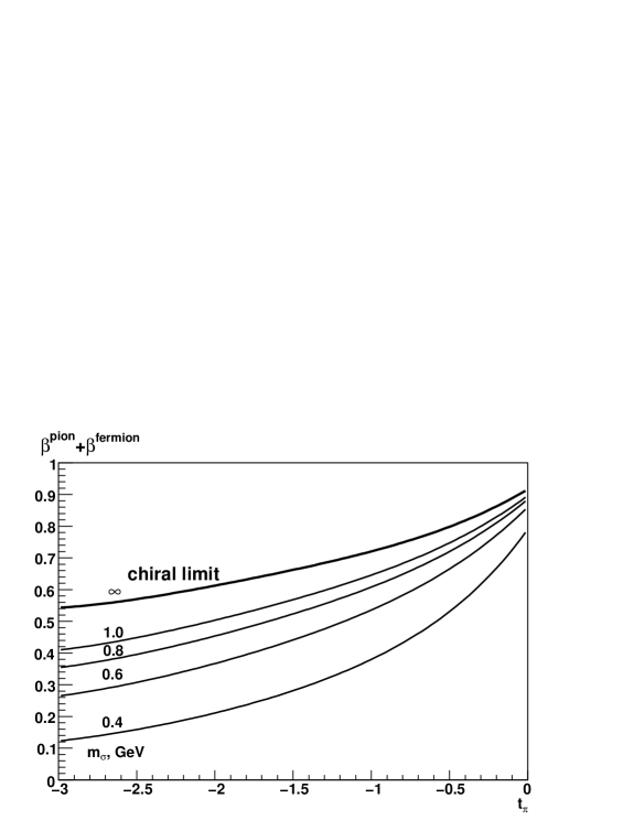
Figure 6: $\beta^{baryon(quark)}+\beta^{pion}$ for different values of $m_{\sigma}$.

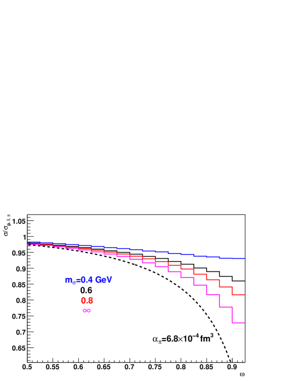
Figure 7: The ratio of the differential cross sections $d\sigma/d\omega$ for different values of $m_{\sigma}$.

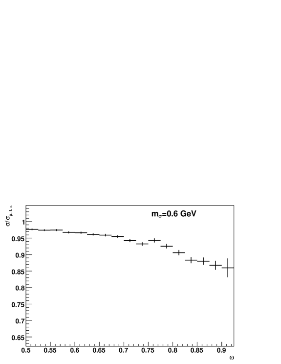
Figure 8: The MC simulation for ratio of the differential cross section $d\sigma/d\omega$ corresponding to 5 months of data taking ($m_{\sigma}=0.6~{}GeV$).

4. Possibility of the experimental test of the prediction of NJL model at COMPASS

The COMPASS is the fixed target experiment in the secondary beam of Super Proton Synchrotron (SPS) at CERN. The purpose of this experiment is the study of hadron structure and hadron spectroscopy with high intensity muon and hadron beams. The COMPASS setup provides unique conditions for investigation of the process (1) ([11],[12],[14],[13]). It has silicon detectors up- and downstream of the target for the precise vertex position reconstruction and for the measurement of the pion scattering angle, an electromagnetic calorimeter for the photon 4-momentum reconstruction and two magnetic spectrometers for the determination of the scattered pion momentum. Hadron calorimeters and muon identification system can be used for identification of secondary particles.

The kinematic range, covered by the COMPASS experiment approximately corresponds to the parameter values range

$$0.5<\omega<0.95,~{}~{}~{}~{}~{}~{}M_{\pi}/3<p_{t}<2M_{\pi},~{}~{}~{}~{}s=(p_{2}+q_{2})^{2}=\frac{M^{2}_{\pi}\omega+p_{t}^{2}}{\omega(1-\omega)}<(3.75M_{\pi})^{2}$$

$$-{2}~{}<~{}\frac{t}{(2m_{\pi})^{2}}<-\frac{1}{8}~{}.$$

The Monte Carlo simulation, based on the realistic description of the COMPASS detector using GEANT3 toolkit, was performed to study the interaction of 190 GeV/c $\pi^{-}$ beam with 5 mm nickel target. High intensity of the hadron beam (up to $2\times 10^{7}$ pions per 10 s spill) and high capabilities of the trigger and DAQ system will allow to collect enough statistics of $\pi^{-}+A\to A+\pi^{-}+\gamma$ events for precise measurement of pion polarizabilities. COMPASS will able to measure the pion polarizabilities not only averaged over some kinematic region (as it was done in Serpukhov experiment [2] and MarkII [4]) but also $\alpha_{\pi}$ dependencies on the kinematic variables.

The possibility to extract the mass of $\sigma$-meson from the behavior of the differential cross section $d\sigma/d\omega$ was studied basing on the assumptions that $\alpha_{E}+\alpha_{H}=0$ and that baryon and pion loops contribute to $\alpha_{\pi^{\pm}}$ (see Fig 6). The ratio of the differential cross section $d\sigma/d\omega$, predicted by NJL model, to the corresponding cross section for point-like pion is presented in Fig. 7. Fig. 8 shows the result of the simulation for $m_{\sigma}=0.6~{}GeV$ for the case of $10^{6}$ events which corresponds to the total beam flux is $4\times 10^{12}$ pions (approximately 5 months of running with beam intensity $2\times 10^{7}$ pions per 10 s spill). The corresponding statistical error of the measurement of the mass of $\sigma$-meson is 25 MeV. For $m_{\sigma}=1.0~{}GeV$ statistical error increases to 90 MeV.

5. Discussion and Conclusion

The charge pion polarizability was considered within the Nambu-Jona-Lazinio model.

In the difference with the earlier papers [8, 25] on the NJL calculation of pion polarizability, where only the quark loops were taken into account, here we calculated the contributions of the meson loops. However, in the case of the Compton effect, the noticeable contribution of the sigma pole diagrams in Figs. 2,3 was strongly concealed by a set of diagrams with internal sigma meson line in Fig. 4.

At the region of transfer $t\ll M^{2}_{\pi}$, the prediction of the NJL model almost coincides within 5 – 10% of accuracy with the QFT approach to Chiral Lagrangian [6], where fermion loops were taking into account.

Thus, the NJL model result reveals the dominant role of the mean field approximation and the sigma pole diagram. This sigma-pole diagram contains the strong t-dependence of the measurable effective polarizability at the region of transfer $t$ of the COMPASS experiment. This t-dependence can explain difference of two experimental results obtained in [2, 3] and by MARK II [4] at the different transverse momentum.

If the experimental uncertainties is less then 5% then pion polarizability dependence on transverse momentum can be measured in the region of the variation of the observable parameters.

6. Acknowledgements

The authors want to thank Drs. A.B. Arbuzov, S.B. Gerasimov, E.A. Kuraev, and M.A. Ivanov for fruitful discussions.

References

• [1] A.Β Klein, Phys.Β Rev.Β  99, 998 (1955).
• [2] Yu M. Antipov et al., Phys. Lett. B 121, 445 (1983);
Yu M. Antipov et al., Z. Phys. C 26, 495 (1985).
• [3] J. Ahrens et al., Eur. Phys. J. A 23, 113 (2005).
• [4] J. Boyer et al., Phys. Rev. D 42, (1990) 1350.
• [5] J.F. Donoghue and B.R. Holstein, Phys. Rev. D 48, 137 (1993).
• [6] M.K. Volkov, V.N. Pervushin. Nuovo Cimento 27A, 277 (1975);
M.K. Volkov, V.N. Pervushin, Sov. J. Part. Nucl. 6 632 (1975);
M.K. Volkov, V.N. Pervushin, Usp. Fiz. Nauk, 120, 363 (1976);
M.K. Volkov, V.N. Pervushin, β€œEssentially Nonlinear Field Theory, Dynamical Symmetry and Meson Physics” ATOMIZDAT, Moscow, ed. D.I.Blokhintsev, 1979 (in Russian).
• [7] V.Β A.Β Petrun’kin, Fiz. Elem. Chastits At. Yadra, 12, 692 (1981).
• [8] M.Β K. Volkov, Sov. J. Part. and Nuclei, 17, 186 (1986).
• [9] L.V. Fil’kov, V.L. Kashevarov, Phys. Rev. C73:035210, (2006); e-Print: nucl-th/0512047; hep-ph/0610102
• [10] J. Gasser, M.A. Ivanov, and M.E. Sainio, Nucl. Phys. B 745, 84 (2006); and refs. therein.
• [11] P. Abbon , E. Albrecht et al., The Compass Experiment at CERN. NIM A577 (2007) 455-518
• [12] M. A. Moinester et al.,Czech.J.Phys.53:B169-B187,2003, hep-ex/0301024
• [13] M. A. Moinester, Pion polarizabilities and Hybrid meson structure at COMPASS, Tel Aviv University Preprint TAUP 2661-2000, hep-ex/0012063
• [14] A. Olchevski, M. Faessler, Experimental requirements for COMPASS Initial Primakoff Physics program, COMPASS coll. Meeting 2001.
• [15] A.S. Galperin, et al. Sov.J. Nucl. Phys. 32, 1053 (1980);
G.M. Mitsel’makher, V.N. Pervushin, Sov. J. Nucl. Phys. 37, 945 (1983).
• [16] V.N. Pervushin, M.K. Volkov. Phys.Lett., 55B, 405 (1975).
• [17] M.K. Volkov, D.I. Kazakov, V.N. Pervushin, T.M.F. 28 46 (1976) (in Russian, translated in English Theor.Math.Phys., 28 27 (1977)).
• [18] S. Weinberg, Phys. Rev. Lett., 18, 188 (1967).
• [19] N. Kaiser, J.M. Friedrich ,Eur. Phys. J.A36:181-188,2008. e-Print: arXiv:0803.0995 [nucl-th]
• [20] J. Gasser and H. Leutweeler, Ann. Phys. (N.Y.) 158, 142 (1984).
• [21] D. Ebert and M.Β K. Volkov, Sov.J. Nucl. Phys. 36, 736 (1982).
• [22] D. Ebert and M.Β K. Volkov, Z. Phys. C 16, 205 (1983).
• [23] Yu.L. Kalinovsky, L. Kaschluhn, V.N. Pervushin. Phys.Lett. 231 B, 288 (1989).
• [24] D. Ebert, H. Reinhardt, and M.Β K. Volkov, Prog. Nucl. Phys. 33, 1 (1994).
• [25] M.Β K. Volkov, A.A. Osipov, Sov. J. of Nucl. Phys., 41, 650 (1985).
• [26] D. Ebert and M.Β K. Volkov, Phys. Lett. 101 B, 252 (1981).
• [27] C.Β Amsler et al., [Particle Data Group], Phys.Β Lett.Β  B 667, 1 (2008).
• [28] D.Β Ebert, T.Β Feldmann and M.Β K.Β Volkov, Int.Β J.Β Mod.Β Phys.Β  A 12, 4399 (1997).
• [29] M.Β K.Β Volkov, Yu.Β M.Β Bystritskiy and E.Β A.Β Kuraev, arXiv:0901.1981 [hep-ph].
• [30] Yu.Β M.Β Bystritskiy, M.Β K.Β Volkov, E.Β A.Β Kuraev, E.Β Bartos and M.Β Secansky, Phys.Β Rev.Β  D 77, 054008 (2008) [arXiv:0712.0304 [hep-ph]].
• [31] M.Β K. Volkov, Ann. Phys. (N.Y.) 157, 282 (1984).
• [32] D. Ebert and H. Reinhardt, Nucl. Phys. B 271, 188 (1986).
• [33] A.S. Galperin, Yu. L. Kalinovsky, β€œPion Polarizability in the Linear Sigma-Model.” JINR -Report N P2 – 10849, JINR, 1977, Dubna.
• [34] L. Maiani, G. Pancheri and N. Paver, eds., The Second DAFNE Physics Handbook (INFN, Frascati, 1995).