Predicted gamma-ray image of SN 1006 due to inverse Compton emission

Abstract

We propose a method to synthesize the inverse Compton (IC) gamma-ray image of a supernova remnant starting from the radio (or hard X-ray) map and using results of the spatially resolved X-ray spectral analysis. The method is successfully applied to SN 1006. We found that synthesized IC gamma-ray images of SN 1006 show morphology in nice agreement with that reported by the H.E.S.S. collaboration. The good correlation found between the observed very-high energy gamma-ray and X-ray/radio appearance can be considered as an evidence that the gamma-ray emission of SN 1006 observed by H.E.S.S. is leptonic in origin, though the hadronic origin may not be excluded.

1 Introduction

H.E.S.S. and MAGIC projects open the era of the very-high energy (VHE) $\gamma$-ray astronomy in the sense that they can provide for the first time detailed images of various astrophysical objects. VHE $\gamma$-ray emission from supernova remnants (SNRs) is one of the key components in investigation of the processes around strong nonrelativistic shocks, namely, dynamics and structure of the shock itself, magnetic field behavior, and microphysics of charged particles including their injection and acceleration. Observations in this energy domain demonstrate that charged particles are really accelerated in SNRs up to the highest energies observed in galactic cosmic rays.

SNRs with known TeV $\gamma$-ray images include RX J1713.7-3946 (Aharonian et al., 2006, 2007a), Vela Jr. (Aharonian et al., 2005c, 2007b), SN 1006 (Naumann-Godo et al., 2009), RCW86 (Aharonian et al., 2009), IC443 (Albert et al., 2007), W28 (Aharonian et al., 2008a), CTB 37B (Aharonian et al., 2008b), G0.9+0.1 (Aharonian et al., 2005a), MSH 15-52 (Aharonian et al., 2005b). Pulsar-wind nebulae could be the origin of $\gamma$-rays in G0.9+0.1 and MSH 15-52 while the particles accelerated at the forward shock of SNRs are likely to be responsible for emission in the other shell-type SNRs.

The broad-band analysis of the spectra from SNRs is useful to set constraints on model parameters but it still leave open the nature of VHE $\gamma$-ray flux either as leptonic or as hadronic in origin (e.g. RX J1713.7-3946: Aharonian et al., 2006; Berezhko & Völk, 2006). The analysis of the spatial distribution of $\gamma$-ray emission is an additional important channel of the experimental information.

Hadronic $\gamma$-rays arise at the location of the target protons. Rather large density of target protons – as e.g. in molecular clouds – is the condition for the effective hadronic emission in SNRs with high TeV $\gamma$-ray fluxes. The morphology of this type of emission in such SNRs is expected to follow the structures of regions of enhanced density of target protons, not the structures in the SNRs where initial protons are accelerated. In SNRs which are bright in $\gamma$-rays, surface brightness distribution of proton-origin $\gamma$-ray emission may not therefore be expected to follow the radio and/or nonthermal X-ray images of SNRs, like it is observed in IC443, W28 or CTB 37B.

In contrast, the VHE $\gamma$-ray and hard X-ray morphologies are observed to be well correlated in the cases of RX J1713.7-3946, Vela Jr., SN 1006 and possibly RCW86. Thus it could be that TeV $\gamma$-rays reflect the same structures where the radio and nonthermal X-ray emission arise. In this scenario, electrons with energies of tens TeV may be responsible both for the (synchrotron) X-rays with energies of few keV and for the inverse-Compton (IC) $\gamma$-rays with energies of few TeV which are observable by H.E.S.S.

The H.E.S.S. image of SN 1006 reported recently (Naumann-Godo et al., 2009) reveals a very good correlation between X- and $\gamma$-ray maps. Can the correlation between IC $\gamma$-ray and synchrotron X-ray images really be an argument for leptonic origin of VHE $\gamma$-ray emission? In the present paper, we make use of the spatially resolved analysis of the radio and X-ray data of SN 1006 to generate images with the possible appearance that this SNR would acquire if the whole TeV $\gamma$-emission were due to leptonic IC process.

Since the purpose of the present analysis is to be as much model independent as possible, our work is mostly based on experimental results, without involving models of SNR dynamics, electron kinetics and evolution, etc., contrary to what has been carried out in previous approaches to the problem (Reynolds, 1998; Fulbright & Reynolds, 1990; Reynolds, 2004; Orlando et al., 2007; Petruk et al., 2009b). Radio and nonthermal X-ray emission contain information about the accelerated electrons, their distribution inside SNR, maximum energies, etc. The method we propose extracts most of the important properties, which are needed to synthesize an IC $\gamma$-ray image, from the radio and X-ray data. The major exception is the magnetic field (MF). In the absence of observational information about it, we consider three cases of possible MF configurations.

2 Methodology

Let us assume that the energy spectrum of electrons holds the following relation

$$N(E)=KE^{-s}\exp(-E/E_{\mathrm{max}}).$$ (1)

where $N(E)$ is the number of electrons per unit volume with arbitrary directions of motion, $E$ the electron energy, $K$ the normalization of the electron distribution, $s$ the power law index and $E_{\mathrm{max}}$ the maximum energy of electrons accelerated by the shock. This equation neglects small concave-up curvature of the spectrum predicted by efficient shock acceleration but allows us to be in the framework of the methodology of the X-ray spectral analysis (Miceli et al., 2009, srcut model was used). The concavity results in a small bump around $E_{\mathrm{max}}$ which leads mainly to some increase of the IC flux, which we are not interested in. It is not expected to affect the pattern of the gamma-ray brightness obtained with our method. Simpler spectrum $N(E)=KE^{-s}$ is valid for the radio emission. The emissivity due to synchrotron or IC emission is

$$q(\varepsilon)=\int dEN(E)p(E,\varepsilon,[B])$$ (2)

where $p$ is the radiation power of a single electron with energy $E$, $\varepsilon$ is the photon energy. The strength of magnetic field $B$ is involved only in the synchrotron emission process.

The simplest way to reach our goal is to use the delta-function approximation of the single-electron emissivities applied to spectrum Eq. (1). Namely, the special function $F$ appeared in the theory of synchrotron radiation is substituted with

$${\cal F}\left(\frac{\nu}{\nu_{\mathrm{c}}}\right)=\delta\left(\frac{\nu}{\nu_{\mathrm{c}}}-0.29\right)\int\limits_{0}^{\infty}F(x)dx$$ (3)

where $\nu$ is the frequency, $\nu_{\mathrm{c}}(B,E)=c_{1}BE^{2}$ is the characteristic frequency, $c_{1}=6.26\times 10^{18}{\,\rm cgs}$. This results in synchrotron radio and X-ray emissivities with the following dependencies:

$$q_{\mathrm{r}}\propto\nu_{\mathrm{r}}^{-(s-1)/2}KB^{(s+1)/2}$$ (4)

$$q_{\mathrm{x}}\propto\nu_{\mathrm{x}}^{-(s-1)/2}KB^{(s+1)/2}\exp\left[-\left(\frac{\nu_{\mathrm{x}}}{\nu_{\mathrm{break}}}\right)^{1/2}\right]$$ (5)

where $\nu_{\mathrm{break}}$ is

$$\nu_{\mathrm{break}}=\nu_{\mathrm{c}}(B,E_{\mathrm{max}}).$$ (6)

With Eq. (4) and Eq. (5), we approximate the relation between the radio and X-ray synchrotron emissivities:

$$q_{\mathrm{x}}=q_{\mathrm{r}}\left(\frac{\nu_{\mathrm{x}}}{\nu_{\mathrm{r}}}\right)^{-(s-1)/2}\exp\left[-\left(\frac{\nu_{\mathrm{x}}}{\nu_{\mathrm{break}}}\right)^{1/2}\right].$$ (7)

However, exponentially cut off electron distribution Eq. (1) convolved with the $\delta$-function approximation for the single-particle emissivity, Eq. (5), underestimates the synchrotron flux from the same electron distribution convolved with the full single-particle emissivity, Eq. (2), at frequencies $\nu>30\nu_{\mathrm{break}}$ (see Fig. 3 in Reynolds (1998), $\nu_{\mathrm{break}}$ is marked as $\nu_{\mathrm{m}}$ there).

In this paper, we use $\nu_{\mathrm{x}}=2.4{\,\rm keV}=5.8\times 10^{17}{\,\rm Hz}$. The range of $\nu_{\mathrm{break}}$ in SN 1006 is found to be $(0.06\div 1)\times 10^{17}{\,\rm Hz}$ (Miceli et al., 2009). Thus, we are working with $\nu_{\mathrm{x}}\approx(6\div 100)\nu_{\mathrm{break}}$. Using Eq. (7) , we may therefore underestimate the real X-ray flux in $\sim 10$ times in regions where $\nu_{\mathrm{break}}$ is small. Thus, as it is pointed out by Reynolds & Keohane (1999), the approximate Eq. (7) is not robust at highest frequencies.

We suggest therefore an empirical approximation of the numerically integrated synchrotron emissivity Eq. (2), i.e. emissivity of the exponentially cut off electron distribution convolved with the full single-particle emissivity:

$$q_{\mathrm{x}}=q_{\mathrm{r}}\left(\frac{\nu_{\mathrm{x}}}{\nu_{\mathrm{r}}}\right)^{-(s-1)/2}\exp\left[-\beta_{\mathrm{x}}\left(\frac{\nu_{\mathrm{x}}}{\nu_{\mathrm{break}}}\right)^{0.364}\right]$$ (8)

where $\beta_{\mathrm{x}}=1.46+0.15(2-s)$. This approximation is quite accurate. Its errors are less than $18\%$ for $s=1.8\div 2.5$ and $\nu_{\mathrm{x}}\leq 10^{3}\nu_{\mathrm{break}}$.

We assume that VHE $\gamma$-ray emission from SN 1006 is due to IC process in the black-body photon field of the cosmic microwave background. The convolution of the electron distribution Eq. (1) with the $\delta$-function approximation for the single-particle IC emissivity (Petruk, 2009) is also inaccurate to describe the $\gamma$-ray radiation of electrons with energies around $E_{\mathrm{max}}$. Therefore, like in the case of the synchrotron radiation, we use an approximate formula for the IC emissivity, too.

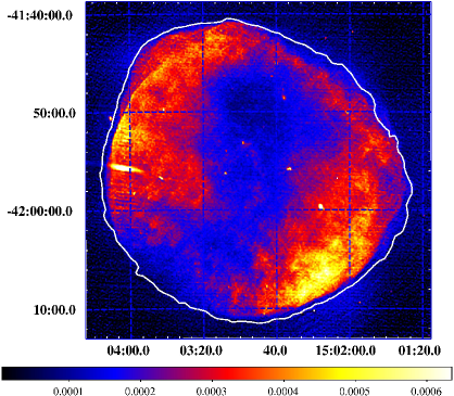
Figure 1: Radio image of SN 1006 at $\lambda\sim 20$ cm. The color scale is in units Jy beam^-1. The white contour denotes the boundary of SN 1006 (see text).

Let us consider IC emission at $1{\,\rm TeV}$. We developed an approximation for the numerically integrated IC emissivity (2) of electrons with the energy spectrum (1) at $\gamma$-ray energy $1{\,\rm TeV}$:

$$q_{\mathrm{ic@1}}\propto K\exp\left(-{\beta_{\mathrm{ic}}}{E_{\mathrm{max}}^{-0.75}}\right)$$ (9)

where $\beta_{\mathrm{ic}}=15$ for $2\leq s\leq 2.5$ and $\beta_{\mathrm{ic}}=15+2(2-s)$ for $1.8\leq s<2$. The error of this approximation is less than $25\%$ for $E_{\mathrm{max}}\geq 0.3{\,\rm TeV}$. This approximation accounts for the Klein-Nishina decline where necessary.

The maximum energy is related to $\nu_{\mathrm{break}}$ by Eq. (6) :

$$E_{\mathrm{max}}=C_{1}\nu_{\mathrm{break}}^{1/2}B^{-1/2}$$ (10)

where $C_{1}=c_{1}^{-1/2}$. Substitution of Eq. (9) with this $E_{\mathrm{max}}$ and $K$ from Eq. (4) results in

$$q_{\mathrm{ic@1}}\propto q_{\mathrm{r}}B^{-(s+1)/2}\exp\left[-\beta_{\mathrm{ic}}\left(\frac{B^{1/2}}{C_{1}\nu_{\mathrm{break}}^{1/2}}\right)^{0.75}\right].$$ (11)

This expression relates the radio emissivity and the IC $\gamma$-ray emissivity at 1 TeV with only one unknown, $B$. It may be used in the same cases where the srcut model is applicable, that is, if the spectrum of electrons may be approximated by Eq. (1) with $s$ assumed constant from the radio to X-ray emitting electrons.

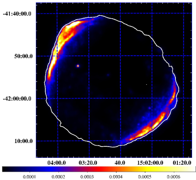
Figure 2: X-ray image of SN 1006 in $2-4.5{\,\rm keV}$. The pixel size is $8^{\prime\prime}$. The color scale is in units MOS1 counts s^-1 pixel^-1.

The idea of our method is represented by Eq. (11). Namely, this expression may be used in a small region (“pixel”) of a SNR projection in order to relate the surface brightness in radio band and IC $\gamma$-rays. Having this relation applied to all “pixels”, we may predict the main features of the $\gamma$-ray morphology of SNR originated in an IC process. This procedure ‘converts’ the radio image to an IC one.

Another possibility is to start from the hard X-ray map and ‘translate’ it into the $\gamma$-ray image in a similar fashion. Namely, substitution Eq. (11) with $q_{\mathrm{r}}$ from Eq. (8) yields

$$\begin{array}[]{l}\displaystyle q_{\mathrm{ic@1}}\propto q_{\mathrm{x}}B^{-(s+1)/2}\exp\left[-\beta_{\mathrm{ic}}\left(\frac{B^{1/2}}{C_{1}\nu_{\mathrm{break}}^{1/2}}\right)^{0.75}\right.\\ \\ \displaystyle\left.\qquad+\beta_{\mathrm{x}}\left(\frac{\nu_{\mathrm{x}}}{\nu_{\mathrm{break}}}\right)^{0.364}\right].\end{array}$$ (12)

However, an X-ray image can be used only if it is dominated everywhere by the nonthermal emission.

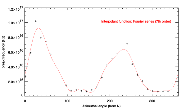
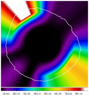
Figure 3: Break frequency $\nu_{\mathrm{break}}$: azimuthal profile (left) and image (right, the color scale is in units of Hz).

Eqs. (11) and (12) relate emissivities of the uniform plasma. We use these equations to deal with surface brightnesses that are superpositions of the local emissivities along the line of sight. Strictly speaking, this may be done only for the thin rim around SNR edge where plasma is approximately uniform along the line of sight. However, this approach may also be extended to deeper regions of SNR projection (see Appendix). Since X-ray limbs are (and $\gamma$-ray ones are expected to be) quite thin and close to the edge, our method is able to correctly determine the location of the bright limbs in the IC $\gamma$-ray image of SN 1006. In the interior of SNR projection, we consider $B$ and $\nu_{\mathrm{break}}$ as ‘effective’ values for a given ‘pixel’.

It is interesting to note that Eq. (11) [or Eq. (12)] may be solved for the value of $B$. In this way, the method proposed here may be used for deriving the effective (line-of-sight averaged) MF pattern in SNR from its radio [or synchrotron X-ray] and IC $\gamma$-ray maps. The distribution of $\nu_{\mathrm{break}}$ may be obtained from the radio ($q_{\mathrm{r}}$) and synchrotron X-ray ($q_{\mathrm{x}}$) images by solving Eq. (8), without the need of the spatially resolved X-ray analysis.

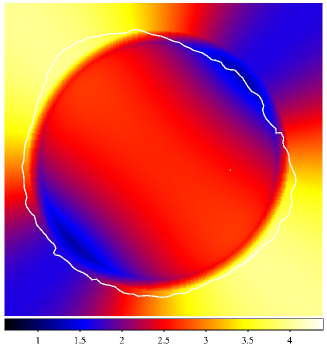
Figure 4: Map of effective MF used in calculations for the model MF1. $\zeta=0.9$. This map is rotated on $90^{\mathrm{o}}$ for the other scenario, MF2. The color scale is in units of $B_{\mathrm{o}}$.

3 Experimental data and models of magnetic field

In order to make use of Eq. (11) or Eq. (12), one needs: i) an initial image, i.e. the map of distribution of the synchrotron radio (or X-ray) surface brightness, ii) the distribution of $\nu_{\mathrm{break}}$ obtained from the spatially resolved spectral analysis of X-ray data and iii) the distribution of the effective magnetic field over the initial image.

We use the high resolution radio image of SN 1006 at $\lambda\sim 20$ cm (Fig. 1), produced on the basis of archival Very Large Array data combined with Parkes single-dish data presented and described in Petruk et al. (2009a).

As for the X-ray image, we use the 2.0-4.5 keV XMM-Newton EPIC mosaic obtained by Miceli et al. (2009), shown in Fig. 2. The mosaic has been produced by combining the 7 public archive XMM-Newton observations of SN1006, and using the PN, MOS1 and MOS2 cameras. The total effective EPIC exposure times ranges between 70 and 140 MOS1-equivalent ks.

A contour plotted on the images delineates the boundary of SN 1006. It corresponds to the level of $10\%$ of the maximum brightness in the soft ($0.5-0.8$ keV) X-ray map of SNR (see Fig. 1 in Miceli et al., 2009).

The azimuthal profile (Fig. 3a) and image (Fig. 3b) of the break frequency was derived on the basis of spatially resolved X-ray spectral fitting results. The reader is referred to Miceli et al. (2009) for the details on the procedure for X-ray data analysis and creation of this image. The same spectral fits also show that $\alpha$, the radio spectral index, is between 0.47 and 0.53 everywhere around the shock. Therefore, we take $s=2\alpha+1=2$ to be constant in SN 1006.

We consider three models for magnetic field inside SNR. SN 1006 is rather symmetrical. In the procedure of MF map simulation, SNR is assumed to be spherical, with the radius equal to the average radius of SN 1006. For technical reasons, MF is fixed to the postshock value also outside the boundary of the spherical SNR (Fig. 4). This allows us to deal correctly also with regions of SN 1006 which are larger than the average radius.

Classical MHD description corresponds to the unmodified shock theory. It takes into account the post-shock evolution of MF and the compression factor which increases with the shock obliquity. In this case, two possible orientations of ISMF are considered. Namely, NW-SE (Fig. 4) in model MF1 (equatorial, or barrel-like, model) and NE-SW in MF2 (polar caps model). ISMF is assumed to be constant around SN 1006 with the strength $B_{\mathrm{o}}=10{\,\rm\mu G}$. This value is choosen to give, in models MF1 and MF2, the postshock magnetic field $20\div 40\ \mu G$, a value which follows from estimations for downstream MF strength (e.g. Völk et al., 2008) and reported $\gamma$-ray flux (Naumann-Godo et al., 2009). Such ISMF looks to be unrealistic at the position of SN 1006 far above the Galactic plane. A possibility to provide tens of $\mu G$ upstream of the shock would be the magnetic field amplificaion as an effect of efficient cosmic ray acceleration, which is out of the scope of this study. It should be noted however that the absolute value of the upstream field plays no role for the purpose of our paper. The aspect angle between ISMF and the line of sight is taken to be $70^{\mathrm{o}}$ for MF1 (Reynolds, 1996; Petruk et al., 2009a) and, for simplicity, also for MF2 (we shall see below that the actual value of the aspect angle is not crucial for the purpose of the present paper, because even different models of MF lead to quite similar $\gamma$-ray pattern).

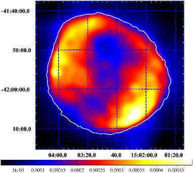
Figure 5: Radio image of SN 1006 at $\lambda\sim 20$ cm, from Fig. 1, smoothed with Gaussian with $2^{\prime}$ sigma.

The procedure of generation of the average MF maps for MF1 and MF2 models is as follows. First we calculated numerically MHD model of Sedov SNR (Sedov, 1959; Reynolds, 1998; Korobeinikov, 1991). This gives us three-dimensional distribution of MF inside SNR. An effective MF in a given ‘pixel’ of SNR projection is taken as a straight average for this 3-D MF distribution along the line of sight, accounting for the azimuthal orientation and an aspect angle of the ambient MF in respect to the observer as well as the fact that most of emission arise right after the shock. Really, in order to generate map of effective MF one should calculate the emissivity-weighted average. Such an approach requires however the knowledge of 3-D distribution of emitting electrons within SNR which is unknown until one makes the full modelling from basic theoretical principles. In contrast, the scope of the present paper is to ‘extract’ the structure of radiating material from the observational data. Therefore, our procedure consists in approximate calculation of emissivity-weighted MF, without considering the 3-D distribution of relativistic electrons. In fact, most emission comes from a rather thin shell with thickness $\sim 10\%$ of SNR radius. Therefore, in calculations of the average magnetic field, we consider only this part of SNR interior, namely the integration along the line of sight is within regions from $\zeta R$ to $R$, with $\zeta<1$ (Fig. 4). A choice of $\zeta$ is rather arbitrary. It is apparent from calculations that contrasts between the outer regions and the interior of the IC image depend on this choice. The preference to the value of $\zeta$ does not alter, however, the main features of the predicted IC morphology of SNR. Note that the azimuthal variation of the brightness is not affected at all by $\zeta$ for radii of SNR projection $\geq\zeta R$. In other words, the position of the limbs on the synthesized IC $\gamma$-ray image may not be altered by the particular choice of $\zeta$. Nevertheless, in order to determine the most appropriate value of $\zeta$, we made the full MHD simulations of Sedov SNR with model of evolution of the relativistic electrons in the SNR interior from Reynolds (1998). Then the map of the emissivity-weighted average MF was produced from these simulations and compared with our maps of effective MF derived for different $\zeta$. In this way, we found that the value $\zeta=0.9$ provides the good correspondence between MF maps in these two approaches.

The third model of MF is relevant to the nonlinear acceleration theory with the time-dependent MF amplification and the high level of turbulence (Bohm limit; Völk et al., 2004). The quasi-parallel theory assumes in this case that the turbulence is produced ahead of the shock, not downstream. The compression of the (already turbulent) magnetic field then does not depend on the original obliquity (Völk et al., 2003; Berezhko et al., 2002). Rakowski et al. (2008) argue that shocks of different initial obliquity subject to magnetic field amplification become perpendicular immediately upstream. ISMF is therefore assumed to increase on the shock by a large factor (due to compression and amplification), the same for any obliquity. In addition, in model MF3, we assume MF to be approximately uniform everywhere inside SNR (Berezhko & Völk, 2004), with the strength $150{\,\rm\mu G}$ (Ksenofontov et al., 2005).

Theoretical work on magnetic-field amplification starting with Bell & Lucek (2001) focuses on shocks which are originally parallel far upstream, with some implications that the process is less effective for (initially) perpendicular shocks. In this scenario, obliquity dependence of the post-shock MF would be opposite to the classical one. Really, MF amplification is expected to follow acceleration efficiency which decrease with the obliquity. If so, limbs in SN 1006 should correspond to the largest post-shock MF. Such MF morphology is qualitatively represented by MF1 model (Fig. 4).

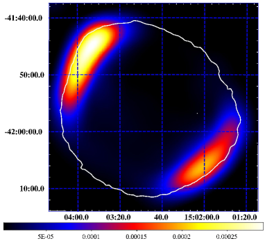
Figure 6: X-ray image of SN 1006 in 2-4.5${\,\rm keV}$, from Fig. 2, smoothed with Gaussian with $2^{\prime}$ sigma.

Some other notes to our methodology are in order. All initial maps were homogenized to the same size, orientation, resolution and pixel size. Eq. (11) is applied to each pixel of the initial images. The maximum brightness on images is fixed at the maximum value in the histogram distribution which has at least 10 pixels. The minimum is fixed at the level 1/100 of the maximum value. This is true for all the images, including the synthesized images, the observed X-ray and radio ones, and excluding the MF and $\nu_{\mathrm{break}}$ maps.

Some images are smoothed to fit the resolution of H.E.S.S. The resolution used is $\mathrm{FWHM}=4.75^{\prime}$ (Aharonian et al., 2005d), so the Gaussian sigma is $2^{\prime}$. The role of smoothing is visible on Figs. 5, 6, to be compared with radio and X-ray images on Figs. 1, 2.

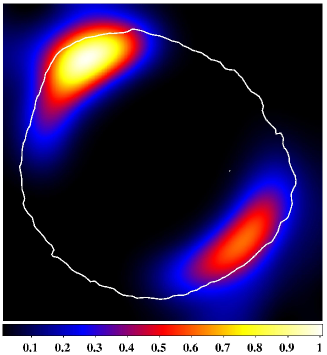
Figure 7: X-ray image of SN 1006 at $2.4{\,\rm keV}$ generated from the radio one (Fig. 1) with the use of Eq. (8) and smoothed to $2^{\prime}$ Gaussian sigma. The color scale is normalized to the maximum brightness.

4 Results and Discussions

To check our approach, we made use of Eq. (8) to generate the X-ray image of SN 1006 starting from the radio one. We stress that we do not need any assumption about MF configuration for this test, everything needed for radio to X-ray conversion may be taken from observations. Really, we need just the input radio image (Fig. 1), and the distribution of the break frequency (Fig. 3). The resulting image is presented on Fig. 7. It shows good correlation with the hard X-ray observations (Fig. 6), confirming that the proposed method works well. It restores the main properties of the observed hard X-ray image: essential decrease of the thickness of the two bright synchrotron limbs in X-rays comparing to the radio band (Fig. 5), correct position of the limbs and negligible emission from the interior. Therefore, the method is reliable to be used for simulation of the $\gamma$-ray images of SNRs.

Synthesized TeV $\gamma$-ray images of SN 1006 due to IC process are presented on Fig. 8 (model MF1, barrel-like SNR in classical MHD or polar caps in non-linear Bell & Lucek (2001) approach), Fig. 9 (MF2, polar-caps in classical MHD) and Fig. 10 (MF3, uniform MF in the SNR interior for Berezhko et al. (2002) non-linear model). Images presented on the left panels were obtained from the radio map as initial model, while those shown in the right panels have the hard X-ray map as the starting point. Middle panels represent ‘radio-origin’ $\gamma$-images of the left panels smoothed to the resolution of H.E.S.S.

Let us first consider the $\gamma$-ray morphologies obtained from the radio image. Two arcs dominate in all three MF configurations. Their locations correspond to limbs in radio and X-ray images. This confirms that correlation between TeV $\gamma$-ray and X-ray/radio morphologies may be considered as direct evidence that the $\gamma$-ray emission of SN 1006 observed by H.E.S.S. is leptonic in origin.

Geometry of MF essentially different from those we considered might result in different predicted $\gamma$-ray images of SNR. Nevertheless, our results demonstrate that if MF strength varies within factor $\sim 3$ around the shock (Fig. 4), any configuration of MF results in double-limb IC $\gamma$-ray image of SN 1006.

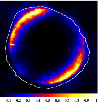
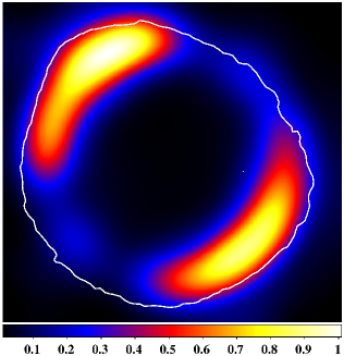
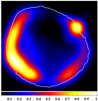
Figure 8: Predicted IC morphology of SN 1006 at photons with energy $1{\,\rm TeV}$, for the model MF1. IC image generated from the radio map (left); the same smoothed to $2^{\prime}$ Gaussian sigma to fit the H.E.S.S. resolution (centre); IC image generated from X-ray map and smoothed to $2^{\prime}$ Gaussian sigma (right). The color scales are normalized to the maximum brightness.

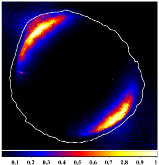
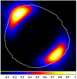
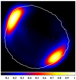
Figure 9: The same as on Fig. 8 for the model MF2.

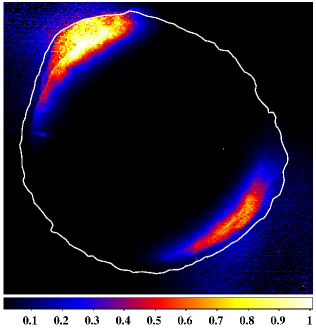
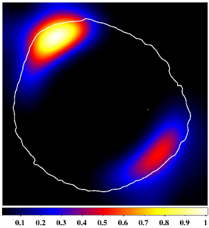
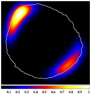
Figure 10: The same as on Fig. 8 for the model MF3.

For areas with the same radio surface brightness, higher MF implies lower IC $\gamma$-ray brightness, Eq. (11). We have therefore different azimuthal contrasts (i.e. the ratio of maximum to minimum brightness around the rim) in $\gamma$-ray images for different models of MF. In particular, in model MF1 the strength of the postshock MF is maximum in NE and SW regions (Fig. 4) where the radio brightness has maxima. At the same time, MF is smaller in faint NW and SE regions. This leads to small azimuthal contrast of brightness between bright and faint regions in $\gamma$-ray image (Fig. 8, left). In the opposite model MF2 the strength of the postshock MF is maximum in the faint NW and SE regions, that results in the largest brightness contrast (Fig. 9, left). Two arcs are therefore more pronounced in the $\gamma$-ray image for models MF2 and MF3.

The differences in $\gamma$-images for three models of MF are not so prominent after smoothing them to the resolution of H.E.S.S. In all three cases (Fig. 8-10, center panels), there are two bright limbs in the same locations corresponding to limbs on the smoothed X-ray map shown in Fig. 6. The synthesized images can be also directly compared to the H.E.S.S. map of SN 1006 (Naumann-Godo et al., 2009). Good correlation between the synthesized and the observed images allows us to prefer leptonic origin of TeV $\gamma$-ray emission of this SNR. The uncertainties introduced in our method by the lack of knowledge of the real MF inside the remnant do not alter this correlation, as it is clearly seen from our synthesized images.

VHE $\gamma$-ray images obtained from the initial hard X-ray map (Fig. 8-10, right panels) are quite similar to those from the initial radio map, except for the configuration MF1. This fact reinforce the goodness of our method. The reason of differences between the ‘radio-origin’ and the ‘X-ray-origin’ $\gamma$-ray images in the MF1 case (Fig. 8right) is the contribution of the thermal X-ray emission to the hard X-ray image which was used, in the SE and NW regions of SN 1006. Namely, our fitting show that the fraction of thermal emission in the overall 2-4.5 keV flux in the SE region is about 50% (Miceli et al., 2009). The prominent but localized NW bright spot is completely dominated by the thermal X-ray emission (Vink et al., 2003). So, the $\gamma$-ray brightness in these regions is overestimated in our synthesized images. This effect is not prominent for MF2 and MF3 configurations because MF is large enough in SE region to visually decrease the brightness there. Thus, the X-ray map may be used as initial one in our method only if it is completely dominated everywhere by the nonthermal emission.

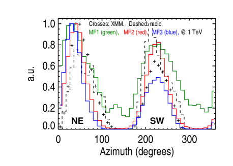
Figure 11: Azimuthal profiles of the observed radio (dashed line) and X-ray (crosses) compared with the synthesized $\gamma$-ray (solid lines) surface brightness (as from the input radio image), from images smoothed with $2^{\prime}$ sigma Gaussian. Background galaxy at the azimuth around $90^{o}$ is excluded.

In order to quantify differences in images due to different models of MF, the azimuthal profiles from our synthesized $\gamma$-ray images are compared on Fig. 11 with the corresponding azimuthal profiles derived from the VLA+Parkes radio image (Fig. 5) and the XMM-Newton X-ray image of SN 1006 (Fig. 6). The profiles have been derived from maps smoothed to the HESS resolution. A large (from $8^{\prime}$ to $20^{\prime}$ from center) annulus centered on the remnant is divided in 40 sectors. The values of brightness plotted is obtained by integration inside the sectors. Observational profiles are corrected for the background which is determined inside the central $0^{\prime}-7^{\prime}$ circle.

Fig. 11 shows that the radio azimuthal profile may not be used as a tracer for the azimuthal variation of the IC $\gamma$-ray brightness because it reflects only the changes in MF strength and density of relativistic electrons, while X-ray profile accounts also for the variation of the electron maximum energy which is important for $\gamma$-ray emission as well.

Fig. 11 reveals a very good match between positions and shape of the limbs in the hard X-ray map seen by XMM-Newton and in all synthesized $\gamma$-ray images. If the future reports of the H.E.S.S. collaboration reveal that the profile of VHE $\gamma$-ray brightness in SN 1006 closely match the XMM-Newton X-ray profile, then Fig. 11 could suggests that the preferred model for SN 1006 could be MF2, i.e. the bright limbs in this SNR might be polar caps (Rothenflug et al., 2004) in classical MHD description. However, it seems that statistical errors affecting modern H.E.S.S. data may not allow us to distinguish between the three models of magnetic field. We expect however that direct comparison of the X-ray and $\gamma$-ray observations with more sofisticated simulations (e.g. involving nonuniform ISMF) allows one to find a correct three-dimensional geometry for SN 1006 and ISMF around it.

5 Conclusions

We propose a general method to synthesize an IC $\gamma$-ray image of SNRs from their observed radio map and the results of spatially resolved X-ray spectral analysis, and we apply it to the supernova remnant SN 1006. The method is based on the fact that the surface brightness distribution of the synchrotron radio and X-ray emission of SNRs contains information about the distribution and properties of accelerated electrons which are responsible for the $\gamma$-ray emission as well. We have derived analytical expression to calculate the $\gamma$-ray image from radio or X-ray surface brightness map, Eq. (11). It is used for each pixel of the input image, knowing the surface distribution of $\nu_{\mathrm{break}}$ and assuming some configuration of magnetic field.

X-ray and TeV $\gamma$-ray photons are radiated by electrons with almost the same energies. It seems therefore to be more natural to use the hard X-ray map as input rather than the radio one. However, we show that the contribution from the thermal component in the initial X-ray image may result in incorrect prediction for the IC brightness distribution. Thus, the hard X-ray map may be used only if it is completely dominated everywhere by the nonthermal emission, which is not the case of the XMM-Newton 2.0-4.5 keV image of SN 1006.

On the other hand, the usage of the radio map as input may introduce some errors due to possible change of the spectral index in the electron spectrum. The applicability of the method may be tested by generating a synchrotron X-ray image from the radio one with Eq. (8). If synthesized distribution of X-ray surface brightness correlates well with the observed one (as in the case of SN 1006) then both the srcut model in XSPEC and our method for IC $\gamma$-ray image may be used for a given SNR.

Our synthesized VHE IC $\gamma$-ray images of SN 1006 are quite similar to that reported in the publication of the H.E.S.S. collaboration (Naumann-Godo et al., 2009). This fact favours a leptonic scenario for the TeV $\gamma$-ray emission of this SNR. However a hadronic origin cannot be ruled out in view of the measured ISM densities, consistent with a hadronic scenario (e.g. Ksenofontov et al., 2005). If this is the case, the observed TeV brightness map may reflect the distribution of protons with energies $>2.4{\,\rm TeV}$ which interact with compressed ISM downstream of the shock.

The present spatial resolution achieved by H.E.S.S., prevents us to ultimately disentangle between the three considered configurations of MF in SN 1006: in all three cases, the two arcs on our $\gamma$-ray images are in the same location as in radio and X-rays. If MF strength varies no more than factor $\sim 3$ or so (as on Fig. 4) around the shocks, IC $\gamma$-ray image of SN 1006 should have two limbs located in the same regions as in X-ray map, independently of the actual azimuthal configuration of MF. The reason, in accordance with Eq. (11), is the contrasts in (radio or X-ray) brightness and $\nu_{\mathrm{break}}$ which dominate any moderate azimuthal variation of MF. The use of the observed ratios of the radio surface brightness and the break frequency between NE and SE regions in Eq. (11) shows that a variation of MF $B_{\mathrm{NE}}/B_{\mathrm{SE}}$ larger than a factor of 4 may reverse the location of bright IC limbs.

Appendix A Approximate description of surface brightness

Here, the approach developed in Petruk et al. (2009a, b) is adopted for general description of the surface brightness. The surface brightness of a spherical SNR projection at distance $\varrho$ from the center and at azimuth $\varphi$ is

$$S(\varrho,\varphi)=2\int^{R}_{a(\varrho)}q(a,\Theta_{\mathrm{o}}){rr_{\mathrm{a}}da\over\sqrt{r^{2}-\varrho^{2}}}.$$ (13)

where $q$ is emissivity, $\Theta_{\mathrm{o}}=\Theta_{\mathrm{o}}(\varphi,r/\varrho,\phi_{\mathrm{o}})$ is the shock obliquity, $\phi_{\mathrm{o}}$ an aspect angle, $r$ and $a$ are Eulerian and Lagrangian coordinates, $r_{\mathrm{a}}$ the derivative of $r(a)$ in respect to $a$. The emissivity in synchrotron or IC process is

$$q=\int dEN(E)p(E,\nu).$$ (14)

In the $\delta$-function approximation of the single-electron emissivity $p(E,\nu)$, we may write that

$$q\propto N(E_{\mathrm{m}})B^{\mathrm{x}}$$ (15)

where $E_{\mathrm{m}}$ is an energy of electron which gives maximum contribution to radiation at a given frequency $\nu$, $\mathrm{x}=1/2$ for synchrotron and $\mathrm{x}=0$ for IC emission.

Energy spectrum of electrons $N(E)$ evolves in a different way downstream of the shocks with different obliquity, i.e. $N(E_{\mathrm{m}})=N(E_{\mathrm{m}};a,\Theta_{\mathrm{o}})$. In Sedov SNR, this evolution may approximately be expressed by the two independent terms (for details see Petruk et al., 2009a, b)

$$N(E_{\mathrm{m}};a,\Theta_{\mathrm{o}})\approx N_{\mathrm{a}}(a)N_{\mathrm{\Theta}}(\varrho,\Theta_{\mathrm{eff}})$$ (16)

where $\Theta_{\mathrm{eff}}=\Theta_{\mathrm{o}}(\varphi,1,\phi_{\mathrm{o}})$. The similar relation holds for MF: $B(a,\Theta_{\mathrm{o}})\approx B_{\mathrm{s}}(\Theta_{\mathrm{o}})B_{\mathrm{a}}(a)$ where $B_{\mathrm{s}}$ is the immediately post-shock value. This allows Eq. (13) to be written as

$$\begin{array}[]{ll}S(\varrho,\varphi)&\propto\displaystyle N_{\mathrm{\Theta}}(\varrho,\Theta_{\mathrm{eff}})B_{\mathrm{s}}(\Theta_{\mathrm{eff}})^{\mathrm{x}}\\ \\ &\displaystyle\times\int^{R}_{a(\varrho)}\!N_{\mathrm{a}}(a)B_{\mathrm{a}}(a)^{\mathrm{x}}{rr_{\mathrm{a}}da\over\sqrt{r^{2}-\varrho^{2}}}.\end{array}$$ (17)

where integral depends on $\varrho$ only. In other notations,

$$S(\varrho,\varphi)\approx q_{\mathrm{eff}}(\varrho,\varphi)\cdot{\cal I}(\varrho)$$ (18)

where ${\cal I}$ is an integral in (17) devided by $N_{\mathrm{a}}(\varrho)$. The accuracy of this approximate formula increases toward the edge of SNR projection where the bright limbs we are interested in are located.

It is important that the factor ${\cal I}$ does not depend on $E_{\mathrm{m}}$, but only on the coordinate in the projection. This means that ${\cal I}$ is almost the same in a given position of the radio, X- and $\gamma$-ray images and we may use Eqs. (8), (11) and (12) written for emissivities in order to relate surface brightnesses in each ‘pixel’. The factor ${\cal I}$ is also independent of $\varphi$ in this approximation. Therefore, the azimuthal variations of the surface brightness $S$ at a given $\varrho$ may be directly represented by the azimuthal variations of the effective emissivities. This provides justification for discussion in Sect. 4. However, the radial contrasts in brightness should account for the radial changes in ${\cal I}$ which is unknown until one considers detailed 3-D MHD model of SNR.

References

- Aharonian et al. (2005a) Aharonian, F. et al., 2005a, A&A 432, L25
- Aharonian et al. (2005b) Aharonian, F. et al., 2005b, A&A 435, L17
- Aharonian et al. (2005c) Aharonian, F. et al., 2005c, A&A 437, L7
- Aharonian et al. (2005d) Aharonian, F. et al., 2005d, ApJ, 636, 777
- Aharonian et al. (2006) Aharonian, F. et al., 2006, A&A 449, 223
- Aharonian et al. (2007a) Aharonian, F. et al., 2007a, A&A 464, 235
- Aharonian et al. (2007b) Aharonian, F. et al., 2007b, ApJ 661, 236
- Aharonian et al. (2008a) Aharonian, F. et al., 2008a, A&A 481, 401
- Aharonian et al. (2008b) Aharonian, F. et al., 2008b, A&A 486, 829
- Aharonian et al. (2009) Aharonian, F. et al., 2009, ApJ 692, 1500
- Albert et al. (2007) Albert, J. et al. 2007, ApJ 664, L87
- Bell & Lucek (2001) Bell & Lucek, 2001, MNRAS, 321, 433
- Berezhko et al. (2002) Berezhko E., Ksenofontov L., Völk H., 2002, A&A, 395, 943
- Berezhko & Völk (2004) Berezhko, E. G., & Völk, H. J. 2004 A&A, 427, 525
- Berezhko & Völk (2006) Berezhko, E. G., & Völk, H. J. 2006, A&A 451, 981
- Fulbright & Reynolds (1990) Fulbright, M. S., & Reynolds, S. P., 1990, ApJ , 357, 591,
- Korobeinikov (1991) Korobeinikov, V., Problems of Point Blast Theory (Springer-Verlag New York, 1991), 400 p.
- Ksenofontov et al. (2005) Ksenofontov, L. T., Berezhko, E. G., Völk, H. J., 2005, A&A, 443, 973
- Miceli et al. (2009) Miceli, M., Bocchino, F., Iakubovskyi, D. et al. 2009, A&A, accepted, astro-ph/0903.3392
- Naumann-Godo et al. (2009) Naumann-Godo, M., Lemoine-Goumard, M., de Naurois, M., 2009, 44th Rencontres de Moriond Proc., submitted
- Orlando et al. (2007) Orlando, S., Bocchino, F., Reale, F., Peres, G., & Petruk, O., 2007, A&A, 470, 927
- Petruk (2009) Petruk, O. 2009, A&A, 499, 643
- Petruk et al. (2009a) Petruk, O., Dubner, G., Castelletti, G., et al. 2009a, MNRAS, 393, 1034
- Petruk et al. (2009b) Petruk, O., Beshley, V., Bocchino, F., & Orlando, S., 2009b, MNRAS, 395, 1467
- Rakowski et al. (2008) Rakowski, C., Laming, J., Ghavamian, P., 2008, ApJ 684, 348
- Reynolds (1996) Reynolds, S. P., 1996, ApJ 459, L13
- Reynolds (1998) Reynolds, S. P., 1998, ApJ 493, 375
- Reynolds (2004) Reynolds, S. P., 2004, Adv. Sp. Res., 33, 461
- Reynolds & Keohane (1999) Reynolds, S. P. & Keohane, J. W. 1999, ApJ 525, 368
- Rothenflug et al. (2004) Rothenflug R., Ballet J., Dubner G., Giacani E., Decourchelle A., & Ferrando P., 2004, A&A, 425, 121
- Schlickeiser (2002) Schlickeiser, R. Cosmic Ray Astrophysics (Springer, 2002)
- Sedov (1959) Sedov L.I., 1959, Similarity and Dimensional Methods in Mechanics (New York, Academic Press).
- Vink et al. (2003) Vink, J., Laming, J. M., Gu, M. F., Rasmussen, A., & Kaastra, J. S., 2003, ApJ 587, L31
- Völk et al. (2003) Völk H., Berezhko E., Ksenofontov L., 2003, A&A, 409, 563
- Völk et al. (2004) Völk, H.J., Ksenofontov, L., Berezhko, E.G., 2004, A&A 427, 525
- Völk et al. (2008) Völk, H.J., Ksenofontov, L., Berezhko, E.G., 2008, A&A 490, 515