Mixing rate for semi-dispersing billiards with non-compact
cusps
A. Arbieto, R. Markarian, M. J. Pacifico and R. Soares
Abstract.
Since the seminal work of Sinai one studies chaotic
properties of planar billiards tables. Among them is the study of
decay of correlations for these tables. There are examples
in the literature of tables
with exponential and even polynomial decay.
However, until now nothing is known about mixing properties
for billiard tables with non-compact cusps. There is no consensual
definition of mixing for systems with infinite
invariant measure. In this paper we study geometric and ergodic
properties of billiard tables with a
non-compact cusp.
The goal of this text is, using the definition of mixing proposed
by Krengel and Sucheston for systems with invariant infinite measure,
to show that the billiard whose table is constituted by the
-axis and and the portion in the plane below the graph
of is mixing and the speed of mixing is
polynomial.
This work was partially supported by CNPq Brazil, Pronex on Dynamical Systems,
FAPERJ-Cientista do Nosso Estado, E-26/100.588/2007, FAPERJ-Bolsa Nota 10-Proc E-26/100.053/2007,
Prodoc-CAPES and Proyecto PDT 2006-2008. S/C/IF/54/001, Uruguay.
1. Introduction
The planar billiard is the dynamical system defined
by the free motion of a particle in the interior of a domain
(usually called table) subjected to elastic collisions to the boundary of ,
that is, angle of incidence equals angle of reflexion.
In a seminal work, Sinai [22] proved that the billiard map
of a system in a two-dimensional torus with finitely many convex
obstacles is a K-automorphism.
For billiards with non-compact cusps, that generate a dynamical system
with an infinite invariant measure, in [15] Lenci proved an
extension of the results of Katok and Strelcyn [11]
for the infinite measure case and, as an application, he showed
that certain tables with non-compact cusps have hyperbolic
structure, that is, existence of absolutely
continuous local stable and unstable manifolds. Furthermore,
adapting arguments contained in [17], Lenci proved that
these billiards maps are ergodic.
About the finite measure case, in [2],
Bunimovich and Sinai proved a “stretched” exponential decay of correlations
for dispersing billiards.
Young [23] showed that the decay of correlations is actually exponential.
This later result was extended by Chernov [3] for billiards with positive-angle
corners.
In [18], Markarian, based on [24], showed that
billiards in the Bunimovich stadium has polynomial decay of correlations.
More recently, Chernov and Markarian [6] proved that semi-dispersing
billiard tables with compact cusps also have polynomial decay
of correlations.
Improved estimates for correlations in different types of billiard
tables
were also proved by Chernov and Zhang [7].
We are interested in tables of the form where is a three times differentiable bounded convex function,
satisfying the hypotheses (H1) to (H5) listed in Section 2.
Theorem A.
The billiard map defined in a table with a non-compact cusp is
an infinite K-automorphism.
Following Krengel and Sucheston [13], we say that an endomorphism
on a -finite infinite measure space is F-mixing
if for all measurable set with ,
As it was commented before, there is no consensual definition of
mixing for systems with infinite measure. A discussion on different
definitions of mixing for systems with infinite measure was recently
done by Lenci [16].
Parry [19] showed that “an infinite K-automorphism has
countable Lebesgue spectrum” and in [13], Krengel and Sucheston
showed that “if an endomorphism has countable Lebesgue spectrum then this endomorphism is
F-mixing”. Therefore we get
Corollary 1.1.
The billiard map defined in a table with a non-compact cusp is F-mixing.
For a conservative endomorphism on a -finite measure space , we define its
entropy [12] by
In [12, p. 172], Krengel showed that “every conservative K-automorphism
on a -finite measure space has positive entropy”. Hence
Corollary 1.2.
The entropy of the billiard map defined in a table with a non-compact cusp
is positive.
Furthermore we can study the speed of convergence to zero in this definition of
F-mixing. We say that an endomorphism is polynomially F-mixing if
for some “good” (e.g., with piecewise differentiable boundary)
set with and some
. The constant
depends on but the exponent depends only on .
Using in the definition of the table we show
Theorem B.
The billiard map defined in a table with a non-compact cusp is polynomially F-mixing.
2. Definition of the dynamical system
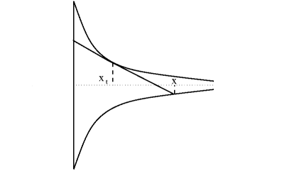
As mentioned in the previous section, we are interested in tables of the form where is a three times differentiable bounded convex function.
Figure 1. Introducing , , e .
We denote by the dispersing part of the table and by the leftmost vertical
wall in .
The angle in the vertex is and it can be zero.
So the billiard table might have a compact cusp besides the non-compact one on
.
We present two other tables, that will be used in the definitions below:
For we use the following notations: indicates
that there exists a constant such that , as ,
analogously for the symbol and we denote by if
tends to zero, as . Moreover, we use the same symbols when ,
if there is no ambiguity.
Also, we indicate by if there exists a constant
such that and
we write if there exists a constant such that .
Define , for each on , implicitly by
One can see that is the -coordinate of the tangent point on .
Figure 2. The point .
In [15], Lenci studied tables with
satisfying the following assumptions
(H1)
as ;
(H2)
;
(H3)
;
(H4)
;
(H5)
, for some
.
It is not difficult to see that satisfies the conditions
above.
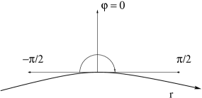
Following [15], choosing as cross-section the rebounds against the dispersing part
. we parametrize these line elements as
, is the arc length variable along (with for
the vertex )
and is the angle between the velocity vector and the normal
at the point of collision, as in Figure 3. We define the manifold
and the return map defined on ,
preserving the measure .
Figure 3. the choice of orientation for and
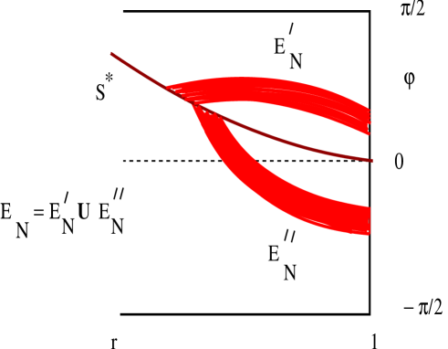
We do not define on those points that hit tangentially or that would end
up in the vertex . That is, we exclude . These points make up
the singularity set of , denoted by . This set consists of two lines
(see [15, p.138]) (as shown in Figure 4).
The curve corresponds to tangencies on in the third
quadrant (on , tangencies on , after a rebound on the vertical side);
this curve is as regular as . As for , its first part corresponds
to line elements pointing to (on , after a rebound on the horizontal side);
as decreases, these become tangencies on . the boundary between these two behaviors
is the only non-regular point of .
Analogously we define , where are the singularity lines
of , obtained from using the time-reversal operator
.
We denote by e .
which will be denoted unstable and stable cones, respectively.
They are strictly invariant under the action of .
Remark 2.1.
We note that our choice of parametrization is different from the one in [15].
This leads to a different choice of the cone bundles.
However, it does not alter the results obtained in that paper.
Let be the leftmost wall on and the phase space defined by
the vectors based on . Since is a global cross-section we can define
a return map and let be the measure
induced on . Denote by the region of located above .
From the definition of , the line elements of are precisely
the ones that,on , hits -axis. We call
the return map to and one can see that
is isomorphic (with respect to ) to .
Lenci [15] showed that the billiard map has a
hyperbolic structure,
i.e., existence of local stable and unstable
manifolds almost everywhere and these local foliations are absolutely
continuous with respect to the invariant measure [15, Theorem 6.2,Theorem 7.5]
and adapting the formulation of Liverani and Wojtkowski [17] to the
infinite measure case, he proved a local ergodicity property [15, Theorem 8.5]
and as consequences its global ergodicity [15, Theorem 8.5].
The definition of ergodicity used in these two results is that the Birkhoff average are constant
almost everywhere for all integrable functions, a weaker definition than the usual one,
for systems with invariant finite measure. However Lenci also proved that
is ergodic [15, Proposition 8.11], which implies that
the billiard map is ergodic in the sense that invariant sets are measurably indecomposable.
Remark 2.2.
It is not difficult to see that is ergodic, for all positive integer .
Indeed, it is just repeated the argument in the proof of [15, Proposition 8.11] .
Next we introduce auxiliary first return maps associated with
the billiard system we are considering. Recall that we already
defined that corresponds for the bouncing at
the vertical wall and corresponding to the
bouncing at the dispersing part of . We point out that a priori,
the bouncing at the dispersing part contains the most of the
chaotic behavior, but this gives a system with an infinity measure,
one of the major difficulties in analyzing this billiard system.
To bypass this difficulty, we consider as well the bouncing at
the vertical wall, that gives a finite measure system. Thus
we set , that consider the bouncing at the dispersing part
and the bouncing at the vertical wall and denote the return map to .
Note that by construction comes from bouncing at a global cross section to
the billiard, constituted by the union of and , the dispersing and the
vertical wall respectively.
Thus is a billiard map that preserves the infinite measure
defined at .
When no ambiguity exists, we will use the same notation for the
(infinite) measure invariant by the map .
Figure 5. The phase space . The line ,
corresponds to the vertex and corresponds
to the vertex in the point of .
As in [15, Corollary 3.3] we conclude that is conservative.
Moreover, since is ergodic and it is induced by ,
so is .
The map describes all the dynamics of our system and this is the map
we shall deal with from now on.
Let be an infinite -finite measure space and
an automorphism. We say that
is an infinite K-automorphism if there exists a sub--algebra such that
(i)
;
(ii)
;
(iii)
.
The next proposition is an extension for K-automorphisms
of a similar result for ergodic maps in spaces with infinite
measure. See [1, p. 42].
Proposition 3.2.
Let be an ergodic measure preserving map of the -finite
measure space and suppose there exists such
that and
.
If is a (finite or infinite) K-automorphism
then is a (finite or infinite) K-automorphism.
Proof.
Since is a K-automorphism, there exists , sub--algebra of
such that
(1)
;
(2)
;
(3)
.
Let . Then
(i) .
(ii) ;
since, by condition (2), ,
and given ,
Because , it follows that
, so
.
Thus .
(iii) We must show that
To do this, we just need to show that
Let and
suppose that .
Furthermore, we may suppose that
because, if not, we take
as the set.
Then which is equal to ,
by the definition of .
By condition (1), ,
so
, by condition (3).
Then
and .
Thus
.
Also, ,
for all .
Then , for all ,
because
.
Since , we get
hence .
∎
We also need the following theorem due to Pesin and
Katok and Strelcyn:
Theorem 3.3.
(Pesin [20, Theorem 7.2] , Katok and Strelcyn [11, Theorem 13.1])
Let be a finite union of compact Riemannian manifolds
(possibly with boundaries and corners),
all of them with dimension , glued along finitely many
submanifolds of positive codimension and a map on
preserving a Borel probability measure , both satisfying the Katok
and Strelcyn conditions indicated in [11, Section 1.1] .
Suppose that
has positive -measure.
Then there exist sets ,
, such that
(1)
, for
, ;
(2)
, , for ;
(3)
for : ,
is ergodic;
(4)
for , there exists a splitting
such that
(a)
for ;
(b)
para ,
;
(c)
is a finite K-automorphism.
Returning to the billiard map case:
Lemma 3.4.
Let be the phase space associated to the rebounds in the vertical wall.
Then is a finite K-automorphism.
Proof.
We know that is ergodic for all . Also, the Lyapunov
exponents for are non-zero. So we may apply Theorem 3.3.
However, by the ergodicity of , all the decompositions are trivial and
we get that is a K-automorphism.
∎
From Proposition 3.2, it follows that an
infinite K-system, concluding the proof of Theorem A.
4. Geometric conditions
This section and the next one are inspired in the
analysis for trajectories in a finite cusp studied
by Chernov and Markarian [6].
We are in the same setting as in the previous sections.
Fix .
Let us study the behavior of a trajectory that leaving
(with coordinates in ),
enters in the cusp, and comes back after rebounds.
In order to do this, we shall adopt a new system of coordinates from now on.
Let , , be the -coordinate associated to the
-th rebound on ,
(where , leaving ),and , , the positive angle
between the trajectory and the tangent at the point of collision with coordinate
().
Define
that is, the -coordinate of the most interior point
inside the cusp.
If then
(4.1)
(4.2)
If then
Lemma 4.1.
Using the notation above,
Proof.
Suppose that, without lost of generality, . Then
On the other hand,
So,
That is,
Now, we must show that and
, for all while the collisions
remain inside the cusp. Indeed, suppose that for it is true and we shall show it
for . Then
By the induction hypothesis, the following holds
So
(4.3)
Using the hypothesis of induction and by (4.3), we get
Thus
Since , for all ,
e
,
as we wish to demonstrate. Thus
∎
Let us now split the trajectories going through the
cusp in three regions. For this, we choose
sufficiently small, that the exact value
is not important,
e.g. .
This choice allows us to make estimates in three different regions,
defining
We call the series of rebounds between and the entering period,
between and the turning period and between
and the exiting period.
Furthermore, consider large enough, e.g. .
From now on, we use the table
defined by .
Until the end of this section, we use the following change of variables:
Lemma 4.2.
We have
so all segments have size of order .
Moreover
(4.4)
and
Also
(4.5)
and
Proof.
For each , we define .
Using the definition of , we obtain
. Also we define
.
Multiplying (4.1) by
and expanding in its Taylor’s series we get
for some constants . This implies that
, for some .
∎
In the proof of Lemma 4.2, we obtained the following
and we shall use the values from now on.
For ,
let be the time between two consecutive collisions
in the billiard table:
Then, using the values above,
for .
Furthermore, if we denote by the curvature of the dispersing part
of the table at the point of collision ,
we have that, as w enter in the cusp ()
since .
We also have that
(4.14)
Moreover
To obtain , we notice that
This last one can be computed as
And to obtain ,
Hence
(4.15)
Remark 4.3.
Due to the reversibility property of the billiard map, all the formulas obtained
above hold for the exiting period as well. So
(4.16)
During the exiting period we can use the countdown index
obtaining asymptotic rates for
, as for example,
, , etc.
5. Hyperbolicity
We use in this section the p-norm, defined by
for vectors of a point .
For billiard maps, the expansion rate of unstable vectors
(i.e., in an unstable cone) in the p-norm is given by
(see [5, p.58]). Here denotes
the curvature of a small arc transverse to the wave
front. For further details we suggest Chernov and Markarian’s book
[4, Chapter IV].
Moreover, for semi-dispersing billiards, unstable vectors are expanded monotonically
in the p-norm, and this is not necessarily true in the Euclidean norm
(see [5, Section 4.4]).
The values can be calculated inductively as
From the equations (4.5) and (4.16),
we know that and , hence they can be arbitrarily close to zero,
which implies that the expansion rate would be extremely high.
However is an increasing function of and .
So if increases,
decreases. In this way, we can obtain an upper bound for the expansion rate
taking lower bounds for and .
Thus we introduce the following assumption
(5.1)
Let
, where
i.e., indicates the amount of rebounds
in the dispersing part before returning to the vertical wall
. So, is the subset of
that return for the first time to after iterations of .
The main goal of this section is to prove the following theorem
Theorem 5.1.
For all , satisfying e ,
Let us denote by .
For ,
(5.2)
Lemma 5.2.
We have that
,
,
,
Proof.
For ,
for some . Suppose that . Then
If is small enough, the expression in parenthesis is positive and
Similarly
Supposing , we get
If is large enough, the expression in parenthesis is negative for large and
completing the induction.
For ,
e
So
We have that
Moreover
So
Thus
On the other hand
There exist constants and such that
and also , because , and
is a bounded sequence.
So
Thus ,
and therefore .
For , using the reversibility property of the billiard map,
for . In particular,
for some and .
Supposing ,
If is small enough, the expression between brackets is positive, for large,
and we obtain that .
Supposing that ,
If is large enough, the expression between brackets is negative, for large,
and we obtain ,
completing the proof.
∎
Let .
This set is as in Figure 6.
It is bounded by curves, denoted by , and ,
and by the line .
The curve is made up of points from that, leaving ,
they hit the dispersing part
tangentially at the first collision. This is a decreasing curve,
since it is a singularity line for for positive values of
until ;
and it is not hard to calculate the slope of this line,
obtaining that it has an horizontal tangency at
Besides, the lines separating and
are constituted of trajectories which the last collision in leaving out
the cusp is tangent. So, they are singularity lines for , and then ,
decreasing lines and regular as consequence of the results in [5, Chapter 4].
Figure 6. The sets , and .
The images
are domains bounded by singularity lines for
, ,
which are curves with positive slope. Moreover, by the property
of time-reversing of the billiard map,
if, and only if,, . So is
obtained reflecting along the line .
The domain close to is made up of two strips:
the inferior strip , which consists of points
that leave the vertical wall and hit the cusp directly;
and the superior strip ,
which consists of points that hit the cusp after a rebound in the horizontal
part of the table . The sets , , make up a nested
structure that shrink to (1,0) as goes to infinity (it is enough
to note that in order to achieve more rebounds inside the cusp, on ,
we must begin closer to the point and the particle must be thrown
almost parallel with respect to the axis ).
The point from farthest from over is at a distance
because on (given by equation (4.4)).
Over , using the values of and obtained in and
, respectively, and a simple geometric construction,
we get that the distance of the strip to the point is .
Since the lines , and are decreasing and has
horizontal tangent on, the “length” of each strip of is .
Now consider an unstable curve inside one of the strips of ,
transverse to the direction of , by the relation between cones
and singularity lines given by condition (C6) from [15, Section 8]. Using the symmetry of , the set
is a line stretching ”from top to bottom” one of the strips of
, therefore, it has “length” .
Using the fact that the derivative of has an expansion rate of
for unstable vectors, given by Theorem 5.1,
we get that .
This is the “width” of each of the strips of .
Since the sets are away from , the measure
is equivalent to the Lebesgue measure on .
Thus,
so
hence has finite measure.
Also the measure of the intersection
can be computed using the symmetry of the sets
and ,
Thus
showing that the speed of decay is at most polynomial.
Acknowledgments
This work corresponds to the Ph.D. thesis of the fourth author, under
the guidance of Maria Jose Pacifico and Roberto Markarian. He thanks
IMERL-Montevideo for the hospitality during certain period while
working on this project.
R. Markarian and R. Soares thank UNAM, Instituto de Matematicas
in Cuernavaca, Mexico, and A. Arbieto, R. Markarian and
R. Soares thank ICTP-Trieste for their kind hospitality and
financial support during a visit there while working on this project.
M.J. Pacifico thanks Scuola Normale Superiore di Pisa for its kind
hospitality during her staying for a postdoctoral program, when this
work was finished.
Appendix A Mixing systems and another proof of Corollary
1.1
In this section we explain a sufficient condition for a system to be F-mixing.
It is based on the work of Coudene [8]
adapted to our definition of F-mixing. From now on
is a metric space, the Borel -algebra of ,
an infinite -finite regular measure on and a -measure preserving transformation.
Definition A.1.
([8, Definition 1])
We define the stable distribution of of a point as
A measurable function is called -invariant
when there exists a set with full measure such that
for all , implies .
If is invertible we define the unstable distribution
of a point for as the stable distribution
for . In a similar way , we define a -invariant function.
We say that the stable distribution is ergodic if every -invariant function is -almost
everywhere.
The propositions below are slight modifications of Theorem 2 and Theorem 3
from [8]. Indeed, since the main elements used in the proof are
the Banach-Alaoglu Theorem and Banach-Saks Theorem, which are true in Hilbert
spaces, there will be few changes in the proofs. We also assume that the measure is
regular because we use the fact that continuous functions with compact support
are dense in [21, p.69].
Proposition A.2.
(Based on [8, Theorem 2])
Let be a metric space, a regular infinite -finite measure
on , a -measure-preserving transformation
and .
Then any weak limit of is -invariant.
Proof.
Let be a weak limit of . First assume that
is continuous with compact support (thus uniformly continuous). The Banach-Saks
theorem guarantees that there exist subsequences and such that
If , then
So is -invariant.
Let . For all , there exists
a continuous function with compact support such that
.
Passing to a subsequence, by Banach-Alaoglu Theorem,
we can assume that converges weakly to a
function
which is -invariant. It follows that
weakly, which implies that
Thus there exists a sequence of -invariant functions that converges
to in the -norm and, passing to a subsequence,
almost everywhere.
Hence, for a set with full measure, if ,
, we get that
This shows that is -invariant.
∎
Using the proposition above, the next one is proved
as in [8].
Proposition A.3.
(Based on [8, Theorem 3])
Let be a metric space, a regular infinite -finite measure
on , an invertible -measure-preserving transformation
and .
Then any weak limit of is -invariant and -invariant.
Corollary A.4.
If is ergodic then is F-mixing.
Proof.
Let . If has a weak limit,
by Proposition A.2 and hypothesis, this limit
is constant at almost every point; thus it is equal to zero
at almost every point. Therefore is F-mixing.
Suppose that does not converge weakly to zero.
Thus there exist an , a subsequence and a function
such that
However by Banach-Alaoglu Theorem there exists a subsequence such that converges
weakly to a function -invariant, by
Proposition A.2, which is constant by hypothesis and hence
must be zero almost everywhere. This contradiction shows that
is F-mixing.
∎
Take a function which is
-invariant and -invariant. By the property of absolute continuity
of the local stable and unstable manifolds [15], Theorem 7.5,
-invariance and -invariance imply that this function must be constant
almost everywhere in the ergodic component of . However, since
has only one ergodic component
is constant almost everywhere,
that is, and are ergodic. Thus, by Corollary A.4,
is F-mixing
∎
References
[1]J. Aaronson,
“An introduction to infinite ergodic theory”,
Mathematical Surveys and Monographs, 50, American Mathematical Society, Providence, RI, 1997.
[2]L. A. Bunimovich and Ya. G. Sinai,
Statistical properties of Lorentz gas with periodic configuration of scatterers,
Commun. Math. Phys. 78 (1981), 479–497.
[3]N. I. Chernov,
Decay of correlations and dispersing billiards,
J. Statist. Phys. 94(3-4) (1999), 513–556.
[4]N. Chernov and R. Markarian,
“Introduction to the Ergodic Theory of Chaotic Billiards”,
24o Colóquio Brasileiro de Matemática, Publicações
Matemáticas, IMPA, 2003.
[5]N. Chernov and R. Markarian,
“Chaotic billiards”,
Mathematical Surveys and Monographs, 127, American Mathematical Society, Providence, RI, 2006.
[6]N. Chernov and R. Markarian,
Dispersing billiards with cusps: slow decay of correlations,
Commun. Math. Phys. 270 no 3 (2007), 727–758.
[7]N. Chernov and H.-K. Zhang,
Improved estimates for correlations in billiards,
Commun. Math. Phys. 277 no 2 (2008), 305–321.
[8]Y. Coudene,
On invariant distributions and mixing,
Ergod. Th. and Dynam. Sys. 27 (2007), 109–112.
[9]N. A. Friedman,
Mixing transformations in an infinite measure space,
Studies in Probability and Ergodic Theory,
Advances in Mathematics Supplementary Studies, vol 2 (1978), 167–184.
[11]A. Katok, J.-M. Strelcyn, (in collaboration with F. Ledrappier and F.Przytycki),
“Invariant manifolds, entropy and billiards; smooth maps with singularities”,
Lect. Notes in Math., 1222, Spinger-Verlag, 1986.
[12]U. Krengel,
Entropy of conservative transformations,
Z. Wahrscheinlichkeitstheorie und Verw. Gebiete 7 (1967), 161–181.
[13]U. Krengel and L. Sucheston,
On mixing in infinite measure spaces,
Z. Wahrscheinlichkeitstheorie und Verw. Gebiete 13 (1969), 150–164.
[14]K. Krickeberg,
Strong mixing properties of Markov chains with infinite invariant measure,
in “Proc. Fifth Berkeley Sympos. Math. Statist. and Probability (Berkeley, Calif., 1965/66), Vol. II: Contributions to Probability Theory, Part 2” Univ. California Press, Berkeley, Calif (1967), 431–446.
[15]M. Lenci,
Semi-dispersing billiards with an infinite cusp I,
Commun. Math. Phys. 230 no 1 (2002), 133–180.
[16]M. Lenci,
On infinite-volume mixing,
preprint, http://arxiv.org/abs/0906.4059.
[17]C. Liverani and M. Wojtkowski,
Ergodicity in Hamiltonian systems,
Dynamics reported, 130–202,
Dynam. Report. Expositions Dynam. Systems (N.S.), 4, Springer, Berlin, 1995.
[18]R. Markarian,
Billiards with polynomial decay of correlations,
Ergod. Th. Dynam. Sys. 24 (2004), 177–197.
[19]W. Parry,
Ergodic and spectral analysis of certain infinite measure preserving
transformations,
Proc. Amer. Math. Soc. 16 (1965), 960–966.
[20]Ya. B. Pesin,
Lyapunov characteristics exponents and smooth ergodic theory,
Russ. Math. Surv. 32(4) (1977), 55–114.
[21]W. Rudin,
“Real and Complex Analysis”,
WCB/McGraw-Hill, 3rd edition, 1987.
[22]Ya. G. Sinai,
Dynamical systems with elastic reflections,
Russ. Math. Surveys 25 (1970), 137–189.
[23]L. S. Young,
Statistical properties of dynamical systems with some hyperbolicity,
Ann. of Math.(2) 147 no. 3 (1998), 585–650.
[24]L. S. Young,
Recurrence times and rates of mixing,
Israel J. Math. 110 (1999), 153–188.
A. Arbieto, M. J. Pacifico, R. Soares:
Instituto de Matemática,
Universidade Federal do Rio de Janeiro,
C. P. 68.530, CEP 21.945-970,
Rio de Janeiro, R.J., Brazil.
E-mails:
arbieto@im.ufrj.br, pacifico@im.ufrj.br,castijos@gmail.com
R. Markarian:
Instituto de Matemática y Estadística (IMERL),
Facultad de Ingeniería, Universidad de la República,
CC30, CP 11300, Montevideo, Uruguay.
E-mail: roma@fing.edu.uy


![[Uncaptioned image]](/html/0907.0975/assets/x7.png)