Convex Hull of $N$ Planar Brownian Motions: Exact Results and an Application to Ecology

Abstract

We compute exactly the mean perimeter and area of the convex hull of $N$ independent planar Brownian paths each of duration $T$, both for open and closed paths. We show that the mean perimeter $\displaystyle\langle L_{N}\rangle=\alpha_{N}\,\sqrt{T}$ and the mean area $\displaystyle\langle A_{N}\rangle=\beta_{N}\,T$ for all $T$. The prefactors $\alpha_{N}$ and $\beta_{N}$, computed exactly for all $N$, increase very slowly (logarithmically) with increasing $N$. This slow growth is a consequence of extreme value statistics and has interesting implications in ecological context in estimating the home range of a herd of animals with population size $N$.

Ecologists often need to estimate the home range of an animal or a group of animals, in particular for habitat-conservation planning ConsPlan . Home range of a group of animals simply means the two dimensional space over which they typically move around in search of food. There exist various methods to estimate this home range, based on the monitoring of the positions of the animals over a certain period of time Worton . One method consists in drawing the minimum convex polygon enclosing all monitored positions, called the convex hull. While this may seem simple minded, it remains, under certain circumstances, the best way to proceed Folia . The monitored positions, for one animal, will appear as the vertices of a path whose statistical properties will depend on the type of motion the animal is performing. In particular, during phases of food searching known as foraging, the monitored positions can be described as the vertices of a random walk in the plane ERW ; BRW . For animals whose daily motion consists mainly in foraging, quantities of interest about their home range, such as its perimeter and area, can be estimated through the average perimeter and area of the convex hull of the corresponding random walk (Fig. 1). If the recorded positions are numerous (which might result from a very fine and/or long monitoring), the number of steps of the random walker becomes large and to a good approximation the trajectory of a discrete-time planar random walk (with finite variance of the step sizes) can be replaced by a continuous-time planar Brownian motion of a certain duration $T$.

Figure 1: Convex hull of (a) a 7-step random walk starting at $O$ (b) 3 closed Brownian paths.

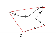
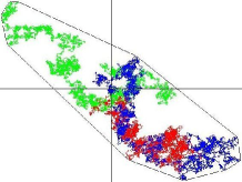
The home range of a single animal can thus be characterized by the mean perimeter and area of the convex hull of a planar Brownian motion of duration $T$ starting at origin $O$. Both ‘open’ (where the endpoint of the path is free) and ‘closed’ paths (that are constrained to return to the origin in time $T$) are of interest. The latter corresponds, for instance, to an animal returning every night to its nest after spending the day foraging in the surroundings. For an ‘open’ path, the mean perimeter $\langle L_{1}\rangle=\sqrt{8\pi T}$ and the mean area $\langle A_{1}\rangle=\pi T/2$ are known in the mathematics literature Ta ; LetacFS ; El . For a ‘closed’ path, only the mean perimeter is known Go : $\langle L_{1}\rangle=\sqrt{\pi^{3}T/2}$.

In any given habitat, an animal is however hardly alone but they live in herds with typically a large population size $N$. To study their global home range via the convex hull model, one needs to study the convex hull of $N$ planar Brownian motions. Assuming that the animals do not develop any substantial interaction between them during foraging, this leads us to the main question addressed in this Letter: what is the mean perimeter and area of the convex hull of $N$ independent planar Brownian motions (both open and closed) each of duration $T$? This question is of vital importance in ecological conservation: if the population size increases by, say ten-fold, by how much should one increase the home range, i.e., the conservation area?

Using the standard scaling property of Brownian motion, ${\rm lengthscale}\sim({\rm timescale})^{1/2}$, it follows that the mean perimeter and area of the global convex hull of $N$ independent Brownian paths will behave as $\langle L_{N}\rangle=\alpha_{N}\sqrt{T}$ and $\langle A_{N}\rangle=\beta_{N}T$ for all $T$. The main challenge is to estimate the $N$-dependence of the prefactors $\alpha_{N}$ and $\beta_{N}$. The central result of this Letter is to provide exact formulae for $\alpha_{N}$ and $\beta_{N}$ for all $N$, both for open and closed paths.

Most interestingly we find that the mean perimeter and area of the convex hull increases very slowly with $N$ for large $N$: $\alpha_{N}\simeq 2\pi\sqrt{2\ln N}$, $\beta_{N}\simeq 2\pi\ln N$ for open paths, and $\alpha_{N}(c)\simeq\pi\sqrt{2\ln N}$, $\beta_{N}(c)\simeq\frac{\pi}{2}\ln N$ for closed paths, $c$ referring to closed paths. This leads to our main conclusion: the home range increases very slowly with increasing population size. Indeed, the $\ln N$ behaviour of the prefactor $\beta_{N}(c)$ in the mean area indicates that, for instance, a $10$-fold increase in the number of animals in the herd will result, on average, in the addition of only about $3.6\ T$ units of area to the home range of the herd — a good news for conservation.

To proceed, let $I$ denote any set of points on the plane with coordinates $(x_{i},y_{i})$. Let $C$ denote the convex hull of $I$, i.e., the minimal convex polygon enclosing this set.

Figure 2: Support function of a 7-step random walk

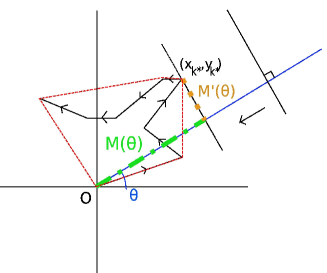
Geometrically, the convex hull can be constructed very simply: consider any arbitrary direction from the origin $O$ specified by the angle $\theta$ with respect to the $x$ axis. Bring a straight line from infinity perpendicularly along direction $\theta$ and stop when it touches a point of the set $I$ [e.g., in Fig. 2, this point has co-ordinates $(x_{k^{*}},y_{k^{*}})$]. Let $M(\theta)$ denote the Euclidean distance of this perpendicular line from the origin when it stops, measuring the maximal extension of the set $I$ along the direction $\theta$. This support function can be simply written as

$$M(\theta)=\max_{i\in I}\left\{x_{i}\cos\theta+y_{i}\sin\theta\right\}.$$ (1)

Knowing $M(\theta)$, one can express the perimeter and the area of the convex hull $C$ via Cauchy’s formulae Cau :

$$L = \int_{0}^{2\pi}d\theta M(\theta)$$ (2)

$$A = \frac{1}{2}\int_{0}^{2\pi}d\theta\left(M^{2}(\theta)-\left(M^{\prime}(\theta)\right)^{2}\right),$$ (3)

where $M^{\prime}(\theta)=dM/d\theta$. In this Letter we show how these two formulae can be used to compute the mean perimeter and area of the convex hull of $N$ planar Brownian motions.

To illustrate the main idea let us start with a single open Brownian path, the generalizations to $N>1$ and for closed paths will follow. In this case the set $I$ consists of the vertices of a Brownian path of duration $T$ starting at the origin $O$. Since it is a continuous path, we can conveniently label the coordinates by $\mathcal{B}(\tau)=(x(\tau),y(\tau))$ with $0\leq\tau\leq T$. Here $x(\tau)$ and $y(\tau)$ are just two independent one dimensional Brownian paths each of duration $T$ and evolve via the Langevin equations: ${\dot{x}}(\tau)=\eta_{x}(\tau)$ and ${\dot{y}}(\tau)=\eta_{y}(\tau)$ where $\eta_{x}(\tau)$ and $\eta_{y}(\tau)$ are independent Gaussian white noises, each with zero mean and delta correlated, e.g., $\langle\eta_{x}(\tau)\eta_{x}(\tau^{\prime})\rangle=\delta(\tau-\tau^{\prime})$ and the same for $\eta_{y}$. Clearly then $\langle x^{2}(\tau)\rangle=\tau$ and $\langle y^{2}(\tau)\rangle=\tau$.

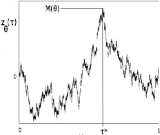
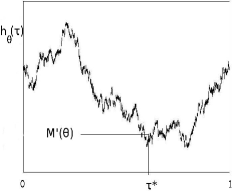
Let us now consider a fixed direction $\theta$. Then, $z_{\theta}(\tau)=x(\tau)\cos\theta+y(\tau)\sin\theta$ and $h_{\theta}(\tau)=-x(\tau)\sin\theta+y(\tau)\cos\theta$ are also two independent one dimensional Brownian motions (each of duration $T$) parametrized by $\theta$. Then $M(\theta)$ in Eq. (1) is simply the maximum of the one dimensional Brownian motion $z_{\theta}(\tau)$ over the time interval $\tau\in[0,T]$, i.e., $M(\theta)={\rm max}[z_{\theta}(\tau)]$. Let $\tau^{*}$ be the time at which this maximum is achieved. Then, $M(\theta)=z_{\theta}(\tau^{*})=x(\tau^{*})\cos\theta+y(\tau^{*})\sin\theta$. Taking derivative with respect to $\theta$ gives $M^{\prime}(\theta)=-x(\tau^{*})\sin\theta+y(\tau^{*})\cos\theta=h_{\theta}(\tau^{*})$. Thus, while $M(\theta)$ is the maximum value of the first Brownian motion $z_{\theta}(\tau)$, $M^{\prime}(\theta)$ is the value of the second independent Brownian motion $h_{\theta}(\tau)$ but at the time $\tau=\tau^{*}$ at which the first one achieves its maximum (see Fig. 3 and 3). Note, in particular, that for $\theta=0$, $z_{0}(\tau)=x(\tau)$ and $h_{0}(\tau)=y(\tau)$. Thus $M(0)$ is the maximum of $x(\tau)$ in $\tau\in[0,T]$ while $M^{\prime}(0)=y(\tau^{*})$ is the value of $y$ at the time $\tau^{*}$ when $x$ achieves its maximum.

Figure 3: (a) Location $\tau^{*}$ of the maximum $M(\theta)$ of $z_{\theta}(\tau)$ and (b) corresponding value of $M^{\prime}(\theta)=h_{\theta}(\tau^{*})$

Taking expectation and using isotropy of the mean over the choice of directions, it follows that

$$\langle L\rangle = 2\pi\ \langle M(0)\rangle$$ (4)

$$\langle A\rangle = \pi\left(\langle[M(0)]^{2}\rangle-\langle[M^{\prime}(0)]^{2}\rangle\right).$$ (5)

For a one dimensional Brownian motion $x(\tau)$ over $[0,T]$, the distribution of its maximum is well known Feller . The cumulative distribution, $Q_{1}(m,T)={\rm Prob}[M(0)\leq m]={\rm erf}(m/\sqrt{2T})$, where ${\rm erf}(z)=\frac{2}{\sqrt{\pi}}\,\int_{0}^{z}e^{-u^{2}}\,du$. The first two moments can be easily computed: $\langle M(0)\rangle=\sqrt{2T/\pi}$ and $\langle[M(0)]^{2}\rangle=T$. Eq. (4) then gives the mean perimeter, $\langle L_{1}\rangle=\alpha_{1}\sqrt{T}$ with $\alpha_{1}=\sqrt{8\pi}$. The calculation of the mean area is slightly trickier since we need $\langle[M^{\prime}(0)]^{2}\rangle$. We first note that for any fixed time $\tau^{*}$, $E[y^{2}(\tau^{*})]=\tau^{*}$ (since it is a free Brownian motion) where the expectation is taken over all realizations of the process $y$ at fixed $\tau^{*}$. But $\tau^{*}$ itself is a random variable, being the time at which the first process $x$ achieves its maximum. Its distribution is also well known and given by the celebrated arcsine law of Lévy Levy : $P(\tau^{*},T)=[\tau^{*}(T-\tau^{*})]^{-1/2}/\pi$. Thus, averaging further over $\tau^{*}$ taken from this distribution, we finally get $\langle[M^{\prime}(0)]^{2}\rangle=\langle\tau^{*}\rangle=T/2$. Eq. (5) then gives the exact mean area $\langle A_{1}\rangle=\beta_{1}T$ with $\beta_{1}=\pi/2$.

For a single closed path, the analysis is similar, except that $x(\tau)$ and $y(\tau)$ are now two independent one dimensional Brownian bridges of duration $T$, i.e., both start at the origin but are constrained to return to the origin at time $T$: $x(0)=x(T)=0$ and $y(0)=y(T)=0$. The distribution of the maximum of a Brownian bridge is also well known Feller and its first two moments are given by: $\langle M(0)\rangle=\sqrt{\pi T/8}$ and $\langle[M(0)]^{2}\rangle=T/2$. Thus, the mean perimeter of the convex hull is given from Eq. (4): $\langle L_{1}\rangle=\alpha_{1}(c)\sqrt{T}$ with $\alpha_{1}(c)=\sqrt{\pi^{3}/2}$. To compute the mean area, we note that for a Brownian bridge $y(\tau)$, at fixed time $\tau^{*}$, $E[y^{2}(\tau^{*})]=\tau^{*}(T-\tau^{*})/T$. Moreover, the distribution of $\tau^{*}$, the time at which a bridge achieves its maximum is known to be uniform Feller . Thus, taking average over $\tau^{*}$ with uniform distribution, $P(\tau^{*},T)=1/T$, we get $\langle M^{\prime}(0)^{2}\rangle=\langle y^{2}(\tau^{*})\rangle=T/6$. Eq. (5) then gives the exact mean area of the convex hull of a planar closed Brownian path: $\langle A_{1}\rangle=\beta_{1}(c)\,T$ with $\beta_{1}(c)=\pi/3$. To our knowledge, this result, even for a single closed path, appears to be new.

This method can then be generalized to $N$ independent planar Brownian paths, open or closed. We now have two sets of $N$ Brownian paths: $x_{j}(\tau)$ and $y_{j}(\tau)$ ($j=1,2,\ldots,N$). All paths are independent of each other. Since isotropy holds, we can still use Eqs. (4) and (5), except that $M(0)$ now denotes the global maximum of a set of $N$ independent one dimensional Brownian paths (or bridges for closed paths) $x_{j}(\tau)$ ($j=1,2,\ldots,N$), each of duration $T$,

$$M(0)=\max_{1\leq j\leq N}\,\max_{0\leq\tau\leq T}\left[x_{1}(\tau),x_{2}(\tau),\ldots,x_{N}(\tau)\right].$$ (6)

Let $j_{*}$ and $\tau^{*}$ denote the label of the path and the time at which this global maximum is achieved. Then, using argument similar to the $N=1$ case, it is easy to see that $M^{\prime}(0)=y_{j_{*}}(\tau^{*})$, i.e., the position of the $j_{*}$-th $y$ path at the time when the $x$ paths achieve their global maximum.

To compute the first two moments of $M(0)$, we first compute the distribution $P_{N}[M(0),T]$ of the global maximum of $N$ independent Brownian paths (or bridges) $x_{j}(\tau)$. This is a standard extreme value calculation. Consider first $N$ open Brownian paths. It is easier to compute the cumulative probability, $Q_{N}(m,T)={\rm Prob}[M(0)\leq m]$. Since the Brownian paths are independent, it follows that $Q_{N}(m,T)=[Q_{1}(m,T)]^{N}$, where $Q_{1}(m,T)={\rm erf}(m/\sqrt{2T})$ for a single path mentioned before. Knowing this cumulative distribution $Q_{N}(M(0),T)$, the first two moments $\langle M(0)\rangle$ and $\langle[M(0)]^{2}\rangle$ can be computed for all $N$. Using the result for $\langle M(0)\rangle$ in Eq. (4) gives us the mean perimeter, $\langle L_{N}\rangle=\alpha_{N}\sqrt{T}$ with

$$\alpha_{N}=4N\sqrt{2\pi}\int_{0}^{\infty}du\ u\ e^{-u^{2}}\left[\text{erf}\left(u\right)\right]^{N-1}.$$ (7)

The first few values are: $\alpha_{1}=\sqrt{8\pi}=5.013..$, $\alpha_{2}=4\sqrt{\pi}=7.089..$, $\alpha_{3}=24\,{\rm tan}^{-1}(1/\sqrt{2})/\sqrt{\pi}=8.333..$ etc. (see Fig. 4 for a plot of $\alpha_{N}$ vs. $N$). For large $N$, one can analyse the integral in Eq. (7) by the saddle point method giving details , $\alpha_{N}\simeq 2\pi\sqrt{2\ln N}$. This logarithmic dependence on $N$ is thus a direct consequence of extreme value statistics Gumbel and the calculation of the mean perimeter of the convex hull of $N$ paths is a nice application of the extreme value statistics.

To compute the mean area, we need to calculate $\langle[M^{\prime}(0)]^{2}\rangle$ in Eq. (5). We proceed as in the $N=1$ case. For a fixed label $j$ and fixed time $\tau$, the expectation $E[y_{j}^{2}(\tau)]=\tau$ which follows from the fact that $y_{j}(\tau)$ is simply a Brownian motion. Thus, $E[y_{j_{*}}^{2}(\tau^{*})]=\tau^{*}$. Next, we need to average over $\tau^{*}$ which is the time at which the global maximum in Eq. (6) happens. The distribution $P_{N}(\tau^{*},T)$ of the time of global maximum of $N$ independent Brownian motions, to our knowledge, is not known in the probability literature. We were able to compute this exactly for all $N$ details . Skipping details, we find that $P_{N}(\tau^{*},T)=\frac{1}{T}\,F_{N}(\tau^{*}/T)$ where

$$F_{N}(z)=\frac{a_{N}}{\sqrt{z(1-z)}}\,\int_{0}^{\infty}dx\,x\,e^{-x^{2}}\,\left[{\rm erf}\left(x\sqrt{z}\right)\right]^{N-1}$$ (8)

and $a_{N}$ is a normalization constant fixed by, $\int_{0}^{1}F_{N}(z)\,dz=1$. It is easy to check that for $N=1$, it reproduces the arcsine law mentioned before. Averaging over $\tau^{*}$ drawn from this distribution, we can then compute $\langle[M^{\prime}(0)]^{2}\rangle=\int_{0}^{T}\tau^{*}P_{N}(\tau^{*},T)\,d\tau^{*}$. Substituting this in Eq. (5) gives the exact mean area for all $N$, $\langle A_{N}\rangle=\beta_{N}T$ with

$$\beta_{N}={4N}\,{\sqrt{\pi}}\,\int_{0}^{\infty}du\ u\ \left[\text{erf}(u)\right]^{N-1}\left(ue^{-u^{2}}-g(u)\right)$$ (9)

where $g(u)=\frac{1}{2\sqrt{\pi}}\int_{0}^{1}\frac{e^{-{u^{2}}/{t}}\ dt}{\sqrt{t(1-t)}}$. For example, the first few values are given by, $\beta_{1}=\pi/2=1.570..$, $\beta_{2}=\pi=3.141..$, $\beta_{3}=\pi+3-\sqrt{3}=4.409..$ etc. (Fig. 4 shows a plot of $\beta_{N}$ vs $N$). The large $N$ analysis gives details , $\beta_{N}\simeq 2\pi\ln N$. Thus for large $N$, the shape of the convex hull approaches a circle of radius $\sqrt{2\ln N}$ which, incidentally, coincides with the set of distinct sites visited by $N$ Brownian motions larralde .

For $N$ closed Brownian planar paths one proceeds in a similar way. Without repeating the analysis, we just mention our main results details . The mean perimeter and area are given by, $\langle L_{N}\rangle=\alpha_{N}(c)\sqrt{T}$ and $\langle A_{N}\rangle=\beta_{N}(c)T$ where, for all $N$,

$$\alpha_{N}(c) = \frac{\pi^{3/2}}{\sqrt{2}}\sum_{k=1}^{N}\binom{N}{k}\frac{(-1)^{k+1}}{\sqrt{k}}$$ (10)

$$\beta_{N}(c) = \frac{\pi}{2}\left[\sum_{k=1}^{N}\frac{1}{k}-\frac{N}{3}+\frac{1}{2}\sum_{k=2}^{N}(-1)^{k}\,f(k)\right]$$ (11)

and $f(k)=\binom{N}{k}\,(k-1)^{-3/2}\left(k\tan^{-1}(\sqrt{k-1})-\sqrt{k-1}\right)$. The first few values are: $\alpha_{1}(c)=\sqrt{\pi^{3}/2}=3.937..$, $\alpha_{2}(c)=\sqrt{\pi^{3}}(\sqrt{2}-1/2)=5.090..$, $\alpha_{3}(c)=\sqrt{\pi^{3}}(3/\sqrt{2}-3/2+1/\sqrt{6})=5.732..$ and $\beta_{1}(c)=\pi/3=1.047..$, $\beta_{2}(c)=\pi(4+3\pi)/24=1.757..$, $\beta_{3}(c)=2.250..$ etc. (see Fig. 4 for a plot of $\alpha_{N}(c)$ and $\beta_{N}(c)$ vs. $N$). Large $N$ analysis shows that details , $\alpha_{N}(c)\simeq\pi\sqrt{2\ln N}$ and $\beta_{N}(c)\simeq\frac{\pi}{2}\ln N$, smaller respectively by a factor $1/2$ and $1/4$ than the corresponding results for open paths.

We have also computed the mean perimeter and area of the convex hull of $N=1,2,3,4$ Brownian paths (both open and closed) via numerical simulations. For each $N$, we constructed $N$ independent normal Gaussian random walks of $10^{4}$ steps each with a time step $\Delta\tau=10^{-4}$. For each realisation of the $N$ walks, we constructed the convex hull using the Graham scan algorithm Graham and computed its perimeter and area and then averaged over $10^{3}$ samples. We find excellent agreement with our analytical predictions (Fig. 4).

Figure 4: Setting $T=1$, the analytical results for average perimeter $\alpha_{N}$ [Eq. (7)] and area $\beta_{N}$ [Eq. (9)] of $N$ open (Op.) Brownian paths, and similarly the average perimeter $\alpha_{N}(c)$ [Eq. (10)] and area $\beta_{N}(c)$ [Eq. (11)] of $N$ closed (Cl.) Brownian paths, plotted against $N$. The symbols denote results from numerical simulations (up to $N=4$).

The method presented here is general and can, in principle, be applied to compute the mean perimeter and area of the convex hull of any set of random points. In fact, when the set consists of just random points, each drawn independently from a given distribution, the statistics of the perimeter and area of their convex hull has been studied extensively in various different contexts Renyi . Our method, using extreme value statistics, can easily recover these results details , but can go further e.g., when the points are correlated as in the case of Brownian paths.

This work leads to several interesting open questions. It would be interesting to extend the results presented here for normal diffusion to the case where the trajectories of animals such as birds, deers or spider monkeys undergo anomalous diffusion, e.g., Lévy flights etc. GM ; KS ; Ramos . Another interesting question concerns the effect of interactions or collective behavior of the animals on the statistics of their convex hulls. For animals like birds that move in $3$-dimensional space, it would be interesting to study the statistics of the convex polytope of their trajectories, such as the mean surface area and the volume of such a polytope details . Finally, the distribution of the time of maximum $\tau^{*}$, a crucial ingredient in our method, has recently been computed exactly for a variety of constrained one dimensional Brownian motions julien . These results may be useful to study the statistics of convex hulls of constrained planar Brownian paths (see e.g.  BL ).

We thank D. Dhar and H. Larralde for useful discussions.

References

- (1) D. Murphy and B. Noon, Ecol. Appl. 2, 3 (1992).
- (2) B.J. Worton, Biometrics 51, 1206 (1995).
- (3) S.A. Boyle et. al. Folia Primatologica 80, 33 (2009).
- (4) F. Bartumeus et. al. Ecology, 86, 3078 (2005).
- (5) H.C. Berg, Random Walks in Biology (Princeton University Press, New York, 1983); L. Edelstein-Keshet, Mathematical Models in Biology (McGraw Hill, Boston, 1988).
- (6) L. Takács, Amer. Math. Month. 87, 142 (1980).
- (7) M. El Bachir Ph.D thesis, Université Paul Sabatier, Toulouse, France 1983.
- (8) G. Letac, J. Theor. Proba. 6, 385 (1993).
- (9) A. Goldman, Prob. Theor. Relat. Fields 105, 57 (1996).
- (10) A. Cauchy, Mem. Acad. Sci. Inst. Fr. 22, 3 (1850); L.A. Santaló, Integral Geometry and Geometric Probability (Addison-Wesley, Reading, MA, 1976).
- (11) W. Feller, An Introduction to Probability Theory and Its Applications ( Wiley, New York, 1968).
- (12) P. Lévy, Compos. Math., 7, 283 (1939).
- (13) Details will be published elsewhere.
- (14) E.J. Gumbel, Statistics of Extremes, (Columbia University Press, New York, 1958).
- (15) H. Larralde et. al. Phys. Rev. A 45, 7128 (1992).
- (16) R.L. Graham, Inform. Proc. Lett. 1,132 (1972).
- (17) A. Rényi and R. Sulanke, Z. Wahrsch. Verw. Geb. 2, 75 (1963).
- (18) G.M. Viswanathan et. al., Nature 381, 413 (1996) (see also A.M. Edwards et. al., Nature 449, 1044 (2007)).
- (19) J. Klafter and I.M. Sokolov, Phys. World 18, 29 (2005).
- (20) G. Ramos-Fernández et. al. Behav. Ecol. Sociobio. 55, 223 (2004).
- (21) J. Randon-Furling and S.N. Majumdar, JSTAT, P10008 (2007); S.N. Majumdar et. al., J. Phys. A: Math. Theor. 41, 365005 (2008).
- (22) P. Biane and G. Letac, arXiv:0905.2256