Investigating the critical properties of beyond-QCD theories using Monte Carlo Renormalization Group matching

Abstract

Monte Carlo Renormalization Group (MCRG) methods were designed to study the non-perturbative phase structure and critical behavior of statistical systems and quantum field theories. I adopt the 2-lattice matching method used extensively in the 1980’s and show how it can be used to predict the existence of non-perturbative fixed points and their related critical exponents in many flavor SU(3) gauge theories. This work serves to test the method and I study relatively well understood systems: the $N_{f}=0$, 4 and 16 flavor models. The pure gauge and $N_{f}=4$ systems are confining and chirally broken and the MCRG method can predict their bare step scaling functions. Results for the $N_{f}=16$ model indicate the existence of an infrared fixed point with nearly marginal gauge coupling. I present preliminary results for the scaling dimension of the mass at this new fixed point.

I Introduction

The Monte Carlo Renormalization Group (MCRG) methods, based on Wilson’s renormalization group theory, were developed and used extensively in the 1980’s to study the critical properties of spin and gauge models Swendsen (1979, 1981, 1984); Hasenfratz et al. (1984a, b); Bowler et al. (1985); Hasenfratz (1984, 1988); Decker et al. (1988); Gupta et al. (1984); Patel and Gupta (1985). The 2-lattice matching MCRG proved to be particularly useful to calculate the $\beta$ function of asymptotically free theories, like quenched QCD Bowler et al. (1985); Hasenfratz et al. (1984a, b). The approach has all but been forgotten in the last 20 years as lattice QCD calculations focused on spectral and other experimentally measurable quantities. Lately there has been increased interest in beyond-QCD lattice models Catterall and Sannino (2007); Appelquist et al. (2008); Shamir et al. (2008); Deuzeman et al. (2008); Del Debbio et al. (2008a); Catterall et al. (2008); Fodor et al. (2008a); Del Debbio et al. (2008b); DeGrand et al. (2009); Hietanen et al. (2009b); Fodor et al. (2008b); Appelquist et al. (2009); Hietanen et al. (2009a); Deuzeman et al. (2009) as they could describe strongly coupled beyond-Standard Model physics Hill and Simmons (2003); Banks and Zaks (1982); Sannino and Tuominen (2005); Dietrich and Sannino (2007). Ref. Fleming (2008) is a good summary of the issues and recent lattice results. A basic discussion of the physical picture with some remarks on expectations for lattice simulations were presented in Ref. DeGrand and Hasenfratz (2009). In this paper I follow the Wilson renormalization group RG language used in DeGrand and Hasenfratz (2009).

SU(3) gauge models with $N_{f}$ fermions in the fundamental representation can have very different phase structure depending on the number of fermions Banks and Zaks (1982). If $N_{f}>16$ asymptotic freedom is lost, the gauge coupling is irrelevant and the continuum theory is free. For small $N_{f}$ the $g=0$, $m=0$ Gaussian fixed point (GFP) is the only critical fixed point (FP). The theory is asymptotically free, confining and chirally broken. Somewhere around $N_{f}\approx 10$ the gauge coupling develops a new FP at $g^{*}\neq 0$ Caswell (1974); Dietrich and Sannino (2007). At $g^{*}$ the gauge coupling is irrelevant, it is an infrared FP (IRFP). The continuum limit defined in the basin of attraction of this IRFP is neither confining not chirally broken; it is conformal when $m=0$. This conformal phase is expected to exits all the way to $N_{f}=16$. Identifying the lower end of the conformal window and the critical properties of the IRFP are the main issues of recent lattice simulations. The MCRG method was designed to answer these kind of questions and in this paper I present the first such study in $N_{f}=4$ and $N_{f}=16$ flavor SU(3) theories. I also investigate the pure gauge SU(3) model where it is possible to do high statistics, large volume simulations. I have chosen these models as the expected phase structure is rather well known, so I can use them to calibrate and test the method. My eventual goal is to extend these studies to other flavor numbers or fermions in different representations.

Since MCRG has been used very little in the last 20 years, I devote Sect.III to the basic description of the 2-lattice matching MCRG. The method allows the determination of a sequence of couplings $\beta_{0},\beta_{1},...\beta_{n},...$ with lattice spacings that differ by a factor of s between consecutive points, $a(\beta_{n})=a(\beta_{n-1})/s$. $s$ is the scale change of the RG transformation, $s=2$ in this study. This sequence is analogous to the step scaling function defined in the Schrodinger functional (SF) method Luscher et al. (1993, 1994); Capitani et al. (1999), but in MCRG it is defined through the bare couplings. To emphasize this difference I will use the notation $s_{b}(\beta_{n};s)=\beta_{n}-\beta_{n-1}$ for the bare step scaling function instead of the more traditional $\sigma(u;s)$ used in the SF approach.

The sequence $\beta_{0},\beta_{1},...\beta_{n},...$ can be used to determine the renormalized running coupling in theories that are governed by the GFP if at the weak coupling end of the chain a renormalized coupling, like the SF $\bar{g}^{2}$, is calculated and connected to a continuum regularization scheme, while at the strong coupling end some physical quantity is used to determine the lattice scale. I do not pursue this calculation here, though I will compare results for $s_{b}(\beta;s=2)$ from SF and MCRG in Sect. IV.1.

The rest of the paper is organized as follows. Sect. II summarizes the perturbative picture of these many fermion theories. Sect. III describes the 2-lattice matching method and defines the RG block transformation used in this work. The numerical simulations and results are discussed in Sect. IV. The technical aspects of MCRG are described in detail for the pure gauge SU(3) theory in Sect.IV.1 as it serves to justify the approach used for the $N_{f}=4$ and $N_{f}=16$ models in Sects. IV.2 and IV.3. I use nHYP smeared staggered fermions in this work. I present some basic properties of 4 flavor staggered fermions, together with the MCRG calculation of the bare step scaling function in Sect. IV.2. The existence of an IRFP requires the re-evaluation of the MCRG method. This, together with preliminary results for the scaling exponent of the mass in the $N_{f}=16$ model are presented in Sect. IV.3.

II The perturbative picture

Before discussing the MCRG method and the numerical results I briefly summarize the perturbative picture. The universal 2-loop $\beta$ function for SU(3) gauge with $N_{f}$ fermions in the fundamental representation is

$$\beta(g^{2})=\frac{dg^{2}}{d\log(\mu^{2})}=\frac{b_{1}}{16\pi^{2}}g^{4}+\frac{b_{2}}{(16\pi^{2})^{2}}g^{6}+\dots\,,$$ (1)

$$b_{1} = -11+\frac{2}{3}N_{f}\,,$$

$$b_{2} = -102+\frac{38}{3}N_{f}\,.$$

For $N_{f}<16.5$ the 1-loop coefficient $b_{1}$ is negative, the gauge coupling is relevant at the $g=0$ Gaussian FP, the theory is asymptotically free. Dimensional transmutation is responsible for mass generation. The energy scale changes by a factor of 2 between couplings $g_{1}$ and $g_{2}$ if

$$\rm{ln}(2)=-\,\int_{g_{1}}^{g_{2}}\frac{g}{\beta(g^{2})}dg\,.$$ (2)

At one loop level this leads to a constant shift in $\beta=6/g^{2}$ and the bare step scaling function is

$$s_{b}(\beta_{1};s=2)=\beta_{1}-\beta_{2}=-\,\frac{3\,\rm{ln}(2)}{4\pi^{2}}b_{1}\,\,\,\,\,\,(\rm{1-loop}).$$ (3)

For small fermion numbers the higher order terms are small, the $\beta$ function is expected to remain negative. Lattice simulations indicate that for $N_{f}\leq 8$ the system is confining and chiral symmetry is spontaneously broken. For $N_{f}>8$ the 2-loop $\beta$ function develops a zero at $g^{*}\neq 0$ Banks-Zaks FPBanks and Zaks (1982). At this new FP $g$ is irrelevant, it is an IRFP for the gauge coupling. The infinite cut-off limit in the vicinity of $g^{*}$ is conformal.

When the perturbatively predicted $g^{*}$ is large, higher order or non-perturbative effects can destroy the existence of the IRFP. Analytical considerations and numerical simulations suggest that the bottom of the conformal window is around $N_{f}\approx 10$ Caswell (1974); Dietrich and Sannino (2007). At $N_{f}=16$, the largest flavor number that is still asymptotically free, the Banks-Zaks FP occours at a small value $g^{*}\sim\epsilon$, perturbation theory could correctly describe the conformal phase. At the IRFP there is only one relevant operator, the mass. Its scaling dimension (critical exponent) is close to its engineering one $y_{m}\sim 1+\cal{O}(\epsilon)$, while the scaling dimension of the gauge coupling is $y_{g}\sim-\epsilon^{2}$. The slope of the $\beta$ function at $g^{*}$ predicts the exponent

$$\beta(g^{2}) = -y_{g}(g^{2}-g^{*2})+{\cal O}((g^{2}-g^{*2})^{2})\,,$$ (4)

$$y_{g} = -\frac{b_{1}^{2}}{b_{2}}\,.$$ (5)

Eq. 2 now gives

$$g_{1}^{2}-g^{*2} = (g_{2}^{2}-g^{*2})2^{-2y_{g}}\,,$$ (6)

$$s_{b}(\beta_{1};s=2) = \beta_{1}-\beta_{2}=(\beta_{2}-\beta^{*})(2^{-2y_{g}}-1)\,,$$ (7)

if $\beta_{1}-\beta^{*}\,,\,\beta_{2}-\beta^{*}\ll 1$. For 16 flavors perturbatively $y_{g}\approx-0.01$, the gauge coupling is almost marginal. For smaller $N_{f}$ or higher representation fermions $|y_{g}|$ can be larger, though both numerical and analytical considerations find that $|y_{g}|$ remains small even at the bottom of the conformal windowGardi and Grunberg (1999); Appelquist et al. (2009); DeGrand and Hasenfratz (2009).

The mass is a relevant operator both at the GFP and at the IRFP, with critical value $m^{*}=0$. Under a scale change $s=2$ it changes as

$$m_{1}=m_{2}2^{-y_{m}}\,,$$ (8)

where $1/y_{m}=\nu$ is the critical index of the mass.

III The MCRG method

The Wilson RG description of statistical systems is a very effective approach to describe the phase diagram, calculate critical indices, and in case of lattice discretized quantum field theories, understand the infinite cut-off continuum limit of these models. There are many books and review articles written about the subject. I do not attempt to explain Wilson RG here, I only summarize the main points. Two reviews that could be useful for other parts of this paper are Refs. Hasenfratz (1984); DeGrand and Hasenfratz (2009).

In the inherently non-perturbative Wilson RG approach one considers the evolution of all the possible couplings under an RG transformation that preserves the internal symmetries of the system but integrates out the cut-off level UV modes. The fixed points of the transformation are characterized by the number of relevant operators, i.e. couplings with positive scaling dimensions that flow away from the FP. Irrelevant couplings have negative scaling dimensions and they flow towards the FP. The IR values of irrelevant operators are independent of their UV values. Continuum (or infinite cut-off) limits can be defined by tuning the relevant couplings towards the FP, thus controlling their IR value. The number of relevant operators and their speed along the RG flow lines are universal, related to the infrared properties of the underlying continuum limit. On the other hand the location of the FP is not physical, in fact different RG transformations have different fixed points.

In quantum field theories the best understood fixed points are at vanishing couplings (Gaussian FPs) as they can be treated perturbatively. For example the GFP of the 4 dimensional SU(3) pure gauge model has one relevant operator, the gauge coupling, and no other FP of the model is known to exist. The Gaussian FP of 2-flavor QCD has two relevant operators, the mass and the gauge coupling. Gauge theories with many flavors can develop, in addition to the GFP, a new fixed point where only the mass is relevant (Banks-Zaks infrared fixed point) Banks and Zaks (1982). These new FPs are rarely in the perturbative region and to study their existence and properties is the main motivation for this paper.

III.1 The 2-lattice matching MCRG method

Consider a $d$-dimensional lattice model with action $S(K_{i})$. $\{K_{i}\}$ denotes the set of all possible couplings, though in a typical lattice simulation only a few of them are non-zero. The system is characterized by one or more length scales, like the correlation length $\xi$, inverse quark masses, etc. In numerical simulations we always deal with finite volume and for now I assume a hypercubic geometry with linear size $L=\hat{L}a$. The first step of a real space renormalization group block transformation is to define block variables. These new variables are defined as some kind of local average of the original lattice variables and for a scale $s>1$ transformation they live on an $\hat{L}/s$ lattice. By integrating out the original variables while keeping the block variables fixed one removes the ultraviolet fluctuations below the length scale $sa$. The action that describes the dynamics of the block variables is usually much more complicated than the original one, but if $s$ is much smaller than the lattice correlation length, the long distance infrared properties of the system are unchanged. After repeated block transformation steps the blocked actions describe a flow line in the multi-dimensional action space

$$\{K_{i}\}\equiv\{K_{i}^{(0)}\}\to\{K_{i}^{(1)}\}\to\{K_{i}^{(2)}\}\to....\,,$$ (9)

where $\{K_{i}^{(n)}\}$ denotes the couplings after $n$ blocking steps. While the physical correlation length is unchanged, the lattice correlation length after $n$ blocking steps is

$$\xi^{(n)} = s^{-n}\xi^{(0)}\,.$$ (10)

The RG can have fixed points only when $\xi=\infty$ (critical) or $\xi=0$ (trivial). We are, of course, interested in the former one. Near the critical fixed point the linearized RG transformation predicts the scaling operators and their corresponding scaling dimensions.

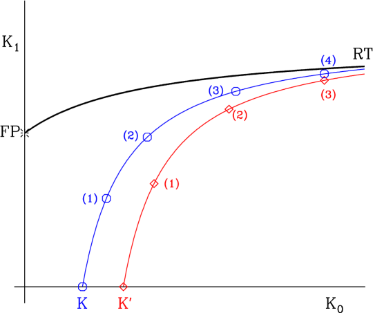
Figure 1: Sketch of the RG flow around a FP with one relevant operator. The coupling pair $(K,K^{\prime})$ indicates matched couplings whose correlation length differ by a factor of $s$.

It is easy to visualize the renormalization group flow lines when there is only one relevant coupling at the fixed point, as illustrated in Fig. 1. The sketch depicts the flow lines in the parameter space $\{K_{0},K_{1}\}$, where for simplicity I assume that the critical surface is at $K_{0}=0$. Flow lines starting near the critical surface approach the fixed point in the irrelevant direction(s) but flow away in the relevant one. After a few RG steps the irrelevant operators die out and the flow follows the unique renormalized trajectory (RT), independent of the original couplings. If we can identify two sets of couplings, $\{K_{i}\}$ and $\{K_{i}^{\prime}\}$, that end up at the same point along the RT after repeated blocking steps, we can conclude that their correlation lengths are identical. If they end up at the same point along the RT but one requires one less blocking steps to do so, according to Eq. 10 their lattice correlation lengths differ by a factor of $s$. This is also illustrated in Fig. 1. From $K^{\prime}$ one needs 3 while from $K$ one needs 4 RG steps to reach the same point of the RT (up to small corrections in the irrelevant direction(s)), therefore $\xi^{\prime}=\xi/s$. This gives the bare step scaling function with scale change $s$. The two lattice matching Hasenfratz et al. (1984b, a) is a numerical method to identify $(K,K^{\prime})$ pairs.

In order to identify a pair of couplings $(K,K^{\prime})$ with $\xi^{\prime}=\xi/s$ we have to show that after $n$ and $(n-1)$ blocking steps their actions are identical, $S(K_{i}^{(n)})=S(K_{i}^{\prime(n-1)})$. It is quite difficult to calculate the blocked action, but fortunately we do not need to know the actions explicitly to shows that they are identical. It is sufficient to show that the expectation values of every operator measured on configurations generated with one or the other action are identical. Furthermore it is possible to create a configuration ensemble with Boltzman weight of an RG blocked action by generating an ensemble with the original action and blocking the configurations themselves Swendsen (1979). This suggests the following procedure for the 2-lattice matching:

1. Generate a configuration ensemble of size $L^{d}$ with action $S(K)$. Block each configuration $n$ times and measure a set of expectation values on the resulting $(L/s^{n})^{d}$ set.

2. Generate configurations of size $(L/s)^{d}$ with action $S(K^{\prime})$, where $K^{\prime}$ is a trial coupling. Block each configuration $n-1$ times and measure the same expectation values on the resulting $(L/s^{n})^{d}$ set. Compare the results with that obtained in step 1. and tune the coupling $K^{\prime}$ such that the expectation values agree.

A few basic comments are in order:

• Since we always compare measurements on the same lattice size, the finite volume corrections are minimal and even very small lattices can be used.

• It is not necessary to work on lattices that are larger than the correlation length of the system, nor does it matter if we are in the confined or deconfined phase of the system.

• If the flow lines follow the unique RT, even one operator expectation value is sufficient to find the matching coupling, all other operators should give the same prediction. In practice we can do only a few blocking steps and the flow lines might not reach the RT. That will be reflected by different operators predicting different matching values. The spread of these predictions measure the goodness of the matching. Increasing the number of blocking steps improves the matching, and when the RT is reached, consequetive blocking steps predict the same matching couplings.

• The location of the fixed point and its renormalized trajectory in the irrelevant directions depend on the block transformation. Block transformations that have free parameters can be optimized so their RT is reached fast and the matching is reliable after a very few RG steps. This optimization proved essential in previous applications Hasenfratz et al. (1984a, b); Bowler et al. (1985); Hasenfratz (1988); DeGrand et al. (1995).

• Since we can match by comparing local operators, the statistical accuracy is usually acceptable even with small configuration sets.

If the FP has two relevant operators, the matching proceeds similarly but one has to tune 2 operators. In practice this is much more difficult than the tuning of a simple coupling. It is frequently easier to fix one of the relevant couplings to its FP value and proceed with the matching in the second relevant coupling as described above.

I will illustrate the above points in Sect.IV.

III.2 The renormalization group block transformation

I chose a scale $s=2$ block transformation, similar to what was used in Refs. Swendsen (1981); Hasenfratz et al. (1984b)

$$V_{n,\mu}={\rm Proj[}(1-\alpha)U_{n,\mu}U_{n+\mu,\mu}+\frac{\alpha}{6}\sum_{\nu\neq\mu}U_{n,\nu}U_{n+\nu,\mu}U_{n+\mu+\nu,\mu}U_{n+2\mu,\nu}^{\dagger}]\,,$$ (11)

where ${\rm Proj}$ indicates projection to $SU(3)$. The parameter $\alpha$ is arbitrary and can be used to optimize the blocking. The block transformation used in Refs. Hasenfratz et al. (1984b); Bowler et al. (1985); DeGrand et al. (1995) had $\alpha$ fixed, $1-\alpha=\alpha/6$, but instead of projecting to SU(3) the blocked link was allowed to fluctuate around $V_{n,\mu}$, depending on a free parameter. In my experience the two block transformations are very similar.

In principle one can define an RG transformation for fermions as well. However it is easier to do the RG transformation after the fermions are integrated out, i.e. when the action depends on the gauge fields only.

The role of the parameter $\alpha$ is to optimize the block transformation. While the critical surface of a system is well defined, the location of the fixed point itself is not physical, it can be changed by changing the RG transformation. It is important to optimize the blocking so its FP and RT can be reached in a few steps. The optimal blocking is characterized by

1. Consistent matching between the different operators: along the RT all expectation values should agree on the matched configuration sets. Any deviation is a measure that the RT has not been reached.

2. Consecutive blocking steps should give the same matching coupling. When they predict different values, one can try to extrapolate to the FP using the first non-leading critical exponent.

In the next Section I will show that both of the above conditions can be satisfied in numerical simulations if the blocking parameter is optimized.

IV Simulations

IV.1 SU(3) pure gauge theory

At the Gaussian $g=0$ FP of the pure gauge SU(3) model the gauge coupling is relevant, the theory is asymptotically free. According to Eq. 3 1-loop perturbation theory predicts that the bare step scaling function is constant, independent of the gauge coupling. The 2-loop corrections are small in a wide range of coupling, $s_{b}^{(\rm{pert})}\approx 0.59$ is a good approximation. The bare step scaling function was studied in Refs.Bowler et al. (1985); Hasenfratz et al. (1984a, b); Gupta et al. (1984) with the 2-lattice matching method. Here I repeat some of those calculations with a different block transformation and extend them to larger volumes and statistics. Where they overlap, the results I present below are consistent with the original calculations. This section mainly serves as a test of the method.

I generated 200-300 independent configurations at several coupling values with the Wilson plaquette gauge action and calculated the bare step scaling function $s_{b}(\beta;s=2)$ matching $32^{4}$ volumes on to $16^{4}$ , and also $16^{4}$ volumes to $8^{4}$. The $32^{4}$ volume can be blocked up to 4 times and compared to the $16^{4}$ volume that is blocked up to 3 times. At each blocking level I measured 5 operators: the plaquette, the 3 6-link loops and a randomly chosen 8-link loop.

Figure 2 illustrates the 2-lattice MCRG. The plot shows the matching of the plaquette with the $s=2$ renormalization group transformation of Eq. 11 and blocking parameter $\alpha=0.65$. The $32^{4}$ volume simulations were done at $\beta=7.0$, and the cyan, blue and red symbols are the values of the blocked plaquette after 2, 3 and 4 blocking steps. The solid curves interpolate the plaquette values, measured at many couplings on $16^{4}$ volumes, after 1, 2 and 3 blocking steps. The $32^{4}$ data match the $16^{4}$ values at $\beta^{\prime}=6.49$ for all blocking levels. The final blocked volume is $2^{4}$, but finite size effects are minimal as one always compares observables on the same volume.

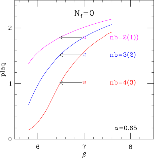
Figure 2: The matching of the plaquette for pure gauge SU(3) theory. The simulations were done on $32^{4}$ volumes at $\beta=7.0$ (symbols) and $16^{4}$ volumes at many coupling values (solid interpolating lines). The configurations were blocked with $s=2$, $\alpha=0.65$ parameter block transformation 2(1) (cyan), 3(2) (blue) and 4(3) times (red).

Figure 3: Matching at $\beta=7.0$ from $32^{4}$ to $16^{4}$ lattices. The matching values $\Delta\beta$ as the function of the blocking parameter $\alpha$ are shown for the 5 different operators measured. Left panel: blocking level $n_{b}=2(1)$; middle panel $n_{b}=3(2)$; right panel $n_{b}=4(3)$.

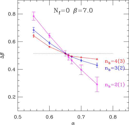
Figure 4: Matching at $\beta=7.0$ from $32^{4}$ to $16^{4}$ lattices. The average matching values $\Delta\beta$ as the function of the blocking parameter for the last 3 blocking levels are shown. Note that the ”error bars” denote the spread of the predictions for the 5 different operators used and thus represent systematical errors.

The matching can be repeated with different operators and RG transformations. Figure 3 shows the difference between the matched couplings,

$$\Delta\beta=\beta-\beta^{\prime}\,,$$ (12)

as the function of the blocking parameter $\alpha$ for the 5 different operators at the last 3 blocking levels for $\beta=7.0$. The plots show two trends. First, the spread of the predicted $\Delta\beta$ values from the different operators decrease with increasing blocking level, signaling that the RG flow lines are approaching the RT of the block transformation. Second, the dependence of $\Delta\beta$ on the blocking parameter decreases with increasing blocking levels suggesting a unique value for $\Delta\beta$ in the $n_{b}\to\infty$ limit.

Figure 4 summarizes the plots of Figure 3. The average matching $\Delta\beta$ values are plotted as the function of $\alpha$ for the last three blocking levels. The “error bars” show the standard deviation (spread) of the predicted values, therefore they represent the systematic errors of the matching procedure. The statistical errors are small, comparable to the systematic errors only at the last blocking level at the best matching around $\alpha=0.65$. The 3 different blocking levels converge around $\alpha=0.65$, the same value where the spread from the different operators is minimal, predicting the relation between the lattice spacings $a(\beta^{\prime}=6.485)=2\,a(\beta=7.0)$. In the $n_{b}\to\infty$ limit the quantity $\Delta\beta(\beta)=\beta-\beta^{\prime}$ is the bare step scaling function $s_{b}(\beta;s=2)$, analogue to the step scaling function of the renormalized coupling used in the SF formalism. In the following I will use the intersection of the last two blocking levels to identify $s_{b}(\beta)$ as it is usually less sensitive to the statistical errors than the spread of the individual operators.

$\beta_{\hat{L}}$	$\alpha_{\rm{opt}}$	$s_{b},\,\hat{L}=32$	$s_{b},\,\hat{L}=32$	$s_{b},\,\hat{L}=16$
		$n_{b}=3(2)$	$n_{b}=4(3)$	$n_{b}=3(2)$
6.0	0.71			0.365(4)
6.2	0.72			0.410(7)
6.4	0.71	0.451(12)	0.448(10)	0.468(16)
6.6	0.69	0.488(15)	0.483(5)	0.496(13)
6.8	0.66			0.511(19)
7.0	0.66	0.517(27)	0.515(6)	0.516(10)
7.2	0.63			0.536(26)
7.4	0.61	0.548(38)	0.571(6)	0.575(42)
7.8	0.60	0.558(34)	0.575(5)	0.573(42)

Table 1: The bare step scaling function for the pure gauge SU(3) system. The second column list the optimal blocking parameter. The third and fourth columns are results from simulations on $32^{4}$ volumes matched to $16^{4}$ after 3(2) and 4(3) blocking steps. The last column shows results from $16^{4}$ volumes matched to $8^{4}$ after 3(2) blocking steps.

Table 1 summarizes the results at different couplings and volumes, together with the optimal blocking parameters $\alpha$. The data indicate consistency between the different volumes and increasing blocking levels. This observation will be important in the study of the $N_{f}=4$ and 16 systems where matching is done on $16^{4}\to 8^{4}$ lattices only. The uncertainty of the predictions from the $16^{4}\to 8^{4}$ are considerably larger than from the larger volumes. This is not statistical, rather reflects the fact that the systematical errors of the matching after 3(2) blocking steps are larger than after one more blocking level. It is possible that a different block transformation would give better matching. I have not been able to modify the scale $s=2$ transformation to make it better. Adding HYP smearingHasenfratz and Knechtli (2001a) before constructing the blocked links pulls the RT closer, but at the same time reduces the dependence of the expectation values on the couplings, thus increasing the errors. It would be worthwhile to try combining the block transformation with a simple APE smearing, or use a variation of the scale $s=\sqrt{3}$ transformation of Refs.Patel and Gupta (1985); Gupta et al. (1984) that would allow more blocking steps from the same lattice size.

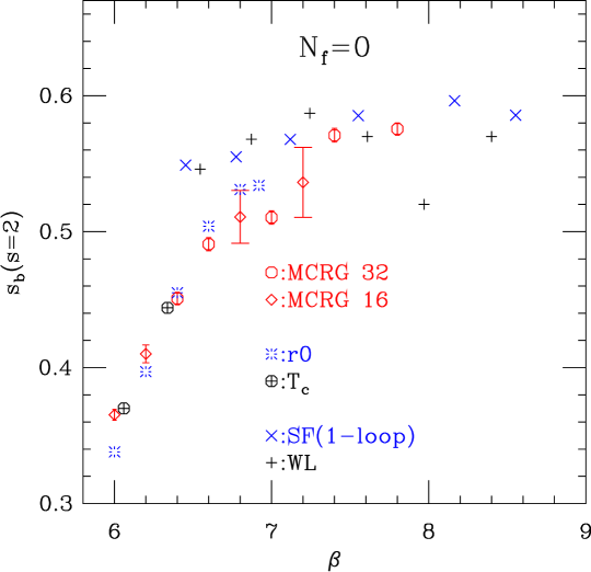
Figure 5: The bare step scaling function $s_{b}(\beta;s=2)$ for the pure gauge SU(3) system as predicted by different methods. The 1-loop perturbative prediction is $s_{b}^{(\rm{pert})}(s=2)=0.59$.

The quantity $s_{b}(\beta;s)$ is the bare step scaling function for scale change $s=2$. One can predict its value using physical observables like the Sommer parameter $r_{0}$Sommer (1994) or the critical temperature $T_{c}$ . The SF calculation or the recently proposed new method to calculate the renormalized coupling based on Wilson loop matching (WL) Bilgici et al. (2009) can also predict $s_{b}(\beta)$.

In Figure 5 I compare the MCRG result for the bare step scaling function with predictions from other methods. Note that I show errors only for the MCRG results. I used the interpolating formula from Ref. Necco and Sommer (2002) to find $(\beta,\beta^{\prime})$ pairs where $r_{0}/a$ differ by a factor of 2, while for $T_{c}$ I used the $N_{T}=8$ and 4, and $N_{T}=12$ and 6 transition temperatures from Ref. Boyd et al. (1996). In case of the SF and WL calculations I attempted to find matching $(\beta,\beta^{\prime})$ pairs by identifying bare couplings where the renormalized SF couplings are related as $\bar{g}^{2}(\hat{L})=\bar{g}^{\prime 2}(2\hat{L})$. In principle this relation should be taken in the $\hat{L}\to\infty$ limit but the numerical data do not show significant finite volume effects. The predictions in Figure 5 use data from the 1-loop improved SF Luscher et al. (1994). The bare couplings used in the 2-loop improved SF paper do not match close enough to use them in this analysis Capitani et al. (1999).

All the above calculations use the Wilson plaquette gauge action, so in the scaling regime they should give the same prediction. It is very satisfying to see the agreement between MCRG, $r_{0}$ and $T_{c}$ even at relatively strong couplings. In the range $\beta\in(6.0,7.0)$ the predicted values differ considerably from the 2-loop perturbative results. It is difficult to measure $r_{0}$ or $T_{c}$ at much finer lattice spacings and show perturbative scaling for them. On the other hand both the SF, WL and MCRG methods approach $s_{b}^{(\rm{pert})}$, but the latter one only at $\beta\geq 7.0$. The relatively large difference between the SF and $r_{0}$ data was discussed and analyzed in Ref. Necco and Sommer (2002) where it was also noted that the 2-loop improved SF shows significantly smaller scaling violations relative to $r_{0}$.

Based on the results presented in this section the 2-lattice MCRG matching method could be competitive with other methods in determining the running coupling of asymptotically free theories when it is combined with an independent definition of the renormalized coupling in the weak coupling regime.

IV.2 $N_{f}=4$ flavor model

The 4 flavor SU(3) gauge theory is expected to be confining and chirally broken even at large gauge couplings. At the Gaussian $g=0,\,m=0$ FP both the mass and the gauge coupling are relevant operators, the model is asymptotically free. Perturbation theory predicts $s_{b}^{(\rm{pert})}(s=2)=0.45$.

The results I present here were obtained using nHYP smeared staggered fermions Hasenfratz et al. (2007). I chose nHYP smearing as it significantly reduces taste breaking of staggered fermions and therefore even in strong coupling has manageable lattice artifacts.

IV.2.1 The nHYP staggered action

Very little is known about the 4-flavor system with nHYP or HYP smeared fermions. The finite temperature phase transition of the HYP smeared model was studied with the partial-global Monte Carlo update in Ref. Hasenfratz and Knechtli (2001b). The phase transition in the chiral limit is expected to be first order, most likely extending to finite mass before turning into a crossover at large masses. Simulations with thin link staggered fermions have confirmed this, finding a strong discontinuity even at fairly large quark masses. The conclusion of Ref. Hasenfratz and Knechtli (2001b) was quite different: we found no signal for discontinuity, the phase transition appeared to be a crossover both for $N_{T}=4$ and 6 even at fairly small masses. The updating technique used in Ref. Hasenfratz and Knechtli (2001b) was not efficient enough to pursue much larger volumes, and we did not continue our investigation of the $N_{f}=4$ system.

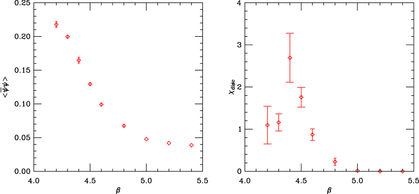
Figure 6: The condensate and the disconnected chiral condensate on $8^{3}\times 4$ volumes at $m=0.04$ in the $N_{f}=4$ theory.

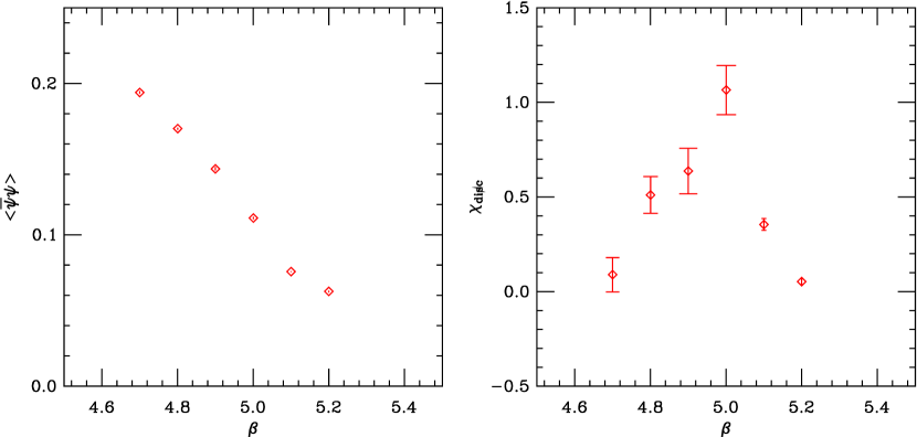
Figure 7: The condensate and the disconnected chiral condensate on $12^{3}\times 6$ volumes at $m=0.05$ in the $N_{f}=4$ theory.

The nHYP smeared action is nearly identical to the HYP smeared one, but nHYP is differentiable and the efficient molecular dynamics update can be used with it Hasenfratz et al. (2007). I have confirmed the raw data of Ref. Hasenfratz and Knechtli (2001b) with the nHYP action, and extended it further toward the strong coupling region. Figure 6 shows the condensate $\langle\bar{\psi}\psi\rangle$ and the disconnected chiral susceptibility Bernard et al. (1996)

$$\chi_{\rm{disc}}=\langle\langle\bar{\psi}\psi\rangle^{2}_{\rm{conf}}\rangle_{U}-\langle\langle\bar{\psi}\psi\rangle_{\rm{conf}}\rangle^{2}_{U}\,$$ (13)

on $8^{3}\times 4$ lattices at $m=0.04$. The condensate is almost identical to Figure 5 of Hasenfratz and Knechtli (2001b), a smooth function of the gauge coupling with no obvious sign of discontinuity. The disconnected chiral susceptibility has a strong peak at $\beta=4.4$, signaling a crossover. In contrast, the data with thin link staggered fermions at $N_{T}=4$ show a discontinuity in the condensate $\Delta\langle\bar{\psi}\psi\rangle\approx 0.2$. Figure 7 is the same as Figure 6 but on $12^{3}\times 6$ lattices at $m=0.05$. Again, the condensate is smooth, the susceptibility suggests a crossover around $\beta=5.0$. Obviously much more work is needed to determine the transition temperatures and the order of the phase transition accurately. Larger spatial volumes might sharpen the transition, but in any case the endpoint of the first order line with nHYP fermions occurs at much smaller masses than with the thin link action.

To set the scale I measured the static potential on $16^{4}$ lattices used later in the MCRG study. I found $r_{0}/a=5.8(3)$ at $\beta=5.4$, $m=0.01$. Ref. Hasenfratz and Knechtli (2001b) quotes $r_{0}/a=3.34(7)$ at $\beta=5.2$, $m=0.04$ and $r_{0}/a=2.2(1)$ at $\beta=5.0$, $m=0.10$.

IV.2.2 MCRG matching

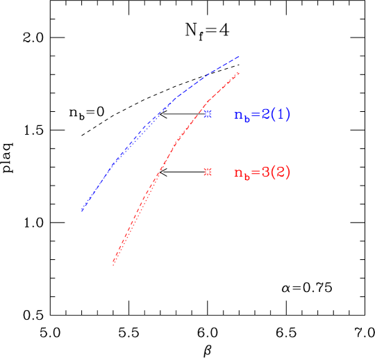
Figure 8: Matching of the plaquette in the $N_{f}=4$ model. The blue and red symbols show the plaquette value after 2 and 3 blocking steps on the $16^{4}$ volumes at $\beta=6.0$, $m=0.01$. The lines interpolate the plaquette on the $8^{4}$ volumes at several couplings and $m=0.015$ (dashed) and $m=0.025$ (dotted) after 1 and 2 blocking levels. The black line is the unblocked plaquette on the $8^{4}$ lattices. The dashed and dotted curves are barely distinguishable.

In principle MCRG matching could be done similarly to the pure gauge SU(3) model, but since the fermionic model has 2 relevant operators, the matching requires tuning in both the gauge coupling and the mass . This is a considerably harder numerical task than a single parameter matching. One can reduce this complication by setting one of the relevant couplings to its critical value, since then only the other coupling has to be matched. The critical value of the mass is $m=0$. Simulations in small volumes are possible even with vanishing mass. In addition the dependence of the local observables used in the matching is so weak on the mass that a small mass in the simulations is also acceptable. Setting the mass to zero or to a small value allows matching in the gauge coupling only and the bare step scaling function can be calculated in the same way as for the pure gauge system.

To calculate the step scaling function I considered $16^{4}\to 8^{4}$ matching at several gauge couplings between $\beta\in(5.4,8.0)$ (see Table 2). All the $16^{4}$ configurations except $\beta=5.4$ are in the deconfined, chirally symmetric phase, but that does not matter for the MCRG matching method. I have generated 100-150 configurations on the larger volumes and $\approx 300$ configurations on the smaller ones, separated by 10 molecular dynamics trajectories. I have used the same 5 operators in the matching as in the pure gauge SU(3) system.

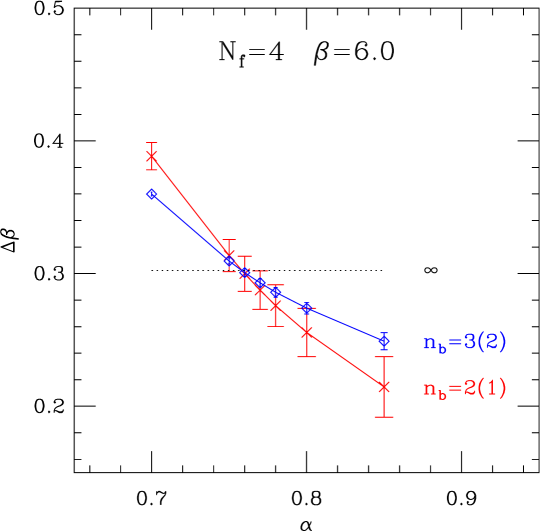
Figure 9: Matching at $\beta=6.0$ from $16^{4}$ to $8^{4}$ lattices in the $N_{f}=4$ model. The matching values $\Delta\beta$ as the function of the blocking parameter for the last 2 blocking levels are shown. Note that the error bars denote the spread of the predictions for the 5 different operators used and thus represent systematical errors.

$\beta_{16}$	$\alpha_{\rm{opt}}$	$s_{b}(s=2)$
5.4	0.81	0.388(10)
5.6	0.81	0.330(13)
5.8	0.77	0.335(20)
6.0	0.76	0.303(25)
6.4	0.67	0.400(29)
6.8	0.67	0.365(42)
7.2	0.63	0.404(39)
8.0	0.59	0.470(53)

Table 2: The bare step scaling function $s_{b}(s=2)$ for the 4-flavor simulation. The second column lists the optimal blocking parameter $\alpha$.

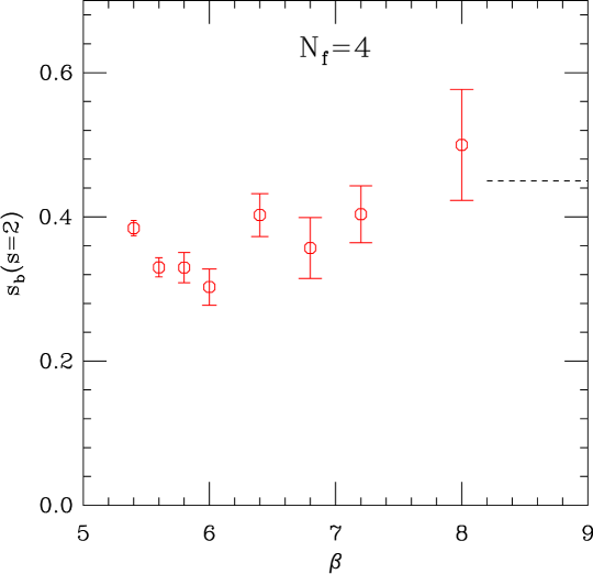
Figure 10: The bare step scaling function for 4 flavor SU(3) theory. The dashed line indicates the 1-loop perturbative value.

On the $16^{4}$ lattices I chose $m=0.01$. If the critical exponent for the mass were its engineering dimension, the matching mass on the smaller volume would be $m=0.02$. I generated $8^{4}$ lattices with $m=0.015$ and 0.025 to bracket this value and to check for any dependence on the mass. The matching for the plaquette is shown in Figure 8. The blue and red symbols represent the plaquette value after 2 and 3 blocking steps on the $16^{4}$ lattice at $\beta=6.0$ while the dashed and dotted lines interpolate the 1 and 2 times blocked plaquette values on the $8^{4}$ lattices with $m=0.015$ and $m=0.025$. For completeness I also show the unblocked plaquette on the $8^{4}$ volumes (black line) though there is no consistent matching at this level. The dotted and dashed curves are barely distinguishable. None of the other observables show any dependence on the mass even after 3 blocking steps beyond the fairly small statistical errors of the simulations, implying that the system indeed can be considered critical in the mass.

The dependence of the matched values on the blocking parameter $\alpha$ is similar to the pure gauge case. The analogue of Figure 4 is Figure 9. Since for $16^{4}\to 8^{4}$ matching only two blocking levels can be used, one has only two sets of predictions, $n_{b}=2(1)$ and $n_{b}=3(2)$. In Sect. IV.1, Table 1 I found that one can safely identify the optimal blocking parameter and matching value from the intersection of these blocking levels even on $16^{4}\to 8^{4}$ matching.

Table 2 and Figure 10 summarize the simulation results. The step scaling function $s_{b}(s=2)$ is consistent with asymptotic freedom and approaches the 2-loop perturbative prediction at weak couplings. Just like in the pure gauge system, the data in Table 2 could be used to determine the running coupling of the 4-flavor model. To do so one needs to calculate a renormalized coupling at $\beta=8.0$ and connect it through perturbation theory to a continuum scheme. The change of the lattice scale between $\beta=5.4$ and $\beta=8.0$ can be determined form the data, while the lattice spacing can be obtained by measuring a physical quantity at some strong coupling. Improved block transformation or larger volumes would allow a more precise determination of $s_{b}(\beta)$. Higher statistics especially at the larger $\beta$ values, would also help.

IV.3 $N_{f}=16$ flavor model

The 16 flavor SU(3) model is still asymptotically free, but 2-loop perturbation theory predicts the emergence of an IRFP at weak gauge coupling Banks and Zaks (1982). Continuum limits can be defined both at the Gaussian FP and at the new IRFP. In the former case both the gauge coupling and the mass has to be tuned towards the FP, in the latter one the gauge coupling is irrelevant, only the mass has to be tuned to $m=0$. There is no confinement or spontaneous chiral symmetry breaking in the weak coupling phase, the continuum massless theory at the IRFP is conformal. The conformal phase was first identified in Ref. Heller (1998).

It is generally believed that in the strong coupling the lattice model is confining and chirally broken, so there has to be a (bulk) transition separating the strong and weak coupling phases. Since the bulk transition is a lattice artifact, it is probably not associated with critical behavior or continuum quantum field theory. Most likely it is a first order phase transition at $m=0$ and it might extend to $m>0$ before turning into a crossover Damgaard et al. (1997); DeGrand and Hasenfratz (2009). One should mention that some numerical results indicate that this confining phase might not even exists Iwasaki et al. (2004).

IV.3.1 MCRG around an infrared fixed point

Assuming that the simulations are done in the conformal phase, the behavior we expect from MCRG depends on whether we study the critical ($m=0$) or the $m\neq 0$ phases:

• On the $m=0$ critical surface at very weak coupling the system is in the attractive region of the Gaussian FP. 2-lattice matching could reveal the running of the gauge coupling, $s_{b}^{(\rm{pert})}=0.016$ from the 1-loop $\beta$ function, though numerical simulations probably will not be close enough to the Gaussian FP to see this behavior. It is much more likely that the RG flow will be determined by the Banks-Zaks IRFP. At this FP all operators are irrelevant when $m=0$. The 2-lattice matching is designed to map out the flow speed in the relevant direction, so we have to re-evaluate the method when there is no relevant operator.

  When all operators are irrelevant, they all flow into the FP according to their scaling dimensions. In the $n_{b}\to\infty$ limit all expectation values approach their FP value independent of the bare couplings, so matching is meaningless. At finite $n_{b}$ the RG flow can pick up the ”least irrelevant” operator. If there is one operator with a nearly zero scaling dimension matching can make sense: after a few RG steps all other operators are already in the FP, so the flow line follows that single operator. According to Eq. 5 the scaling exponent of the gauge coupling for the $N_{f}=16$ flavor theory at the Banks-Zaks FP is small, $\gamma_{g}=-0.01$, it is almost a marginal operator. The scaling exponents of the other irrelevant operators are likely close to their engineering dimensions, starting at $\gamma\approx-2$, so these operators will die out much faster than the gauge coupling.

  The picture we expect in the 2-lattice matching is now clear. Since the gauge coupling is nearly marginal, the matching will follow its flow. $s_{b}(\beta)$ is given by Eq. 7 and for a marginal operator $s_{b}(\beta)=0$ near the FP. For an almost marginal operator $\Delta\beta=\beta-\beta^{\prime}$ can be either positive or negative, depending on whether the FP of the actual RG transformation is at smaller or larger gauge coupling.

  The evolution of the blocked operators can also signal the IRFP. As the RG flow approaches the IRFP all expectation values approach their IRFP value. On the other hand if the GFP controls the system the flow lines follow the RT and run into the trivial $\beta=0$ FP where all local expectation values vanish. This difference is one of the strongest signal for the existence of an IRFP in the MCRG method.

• At finite mass the RG transformation is dominated by the flow of the relevant mass operator. However the nearly marginal gauge coupling can still have a strong influence on the flow, the situation is more like matching 2 relevant operators than matching a single one. The easiest way to deal with this is to set the gauge coupling to its FP value (i.e. to the value that corresponds to the IRFP of the RG transformation used) and match in the mass only. This matching predicts the scaling dimension (or critical exponent) of the mass. While the IRFP of the RG transformation depends on the blocking parameter, the exponent itself is independent of both $\alpha$ and the gauge coupling $\beta$.

IV.3.2 Numerical simulations and results

I concentrate on the renormalization group properties of the model in the massless limit and show only preliminary results at finite mass. I did 2-lattice matching on $16^{4}\to 8^{4}$ lattices using nHYP smeared staggered fermions Hasenfratz et al. (2007), and as in the $N_{f}=4$ case, the simulations were done with a small mass, $m=0.01$ on the $16^{4}$ and $m=0.02$ on the $8^{4}$ lattices. I have collected 100-150 configurations on the larger volumes, $\sim 200$ on the smaller ones, separated by 10 molecular dynamics steps.

On the $8^{4}$ lattices I covered the coupling range $\beta\in(2.4,8)$, trying to identify the bulk transition to the strong coupling phase. The data show no sign of a phase transition, though for $\beta<4.0$ the condensate starts increasing slowly, suggesting the development of spontaneous chiral symmetry breaking. It is likely that the bulk transition exists only at very small, possibly vanishing, mass. This does not contradict the results of Ref. Damgaard et al. (1997) where a strong first order bulk transition was observed with $N_{f}=16$ fermions. As we learned from the finite temperature investigation with $N_{f}=4$ flavors in Sect. IV.2.1, smearing the fermionic action can soften or wash away first order phase transitions, and that might be the situation here as well.

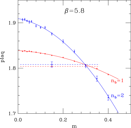
Figure 11: The dependence of the plaquette on the mass after 1 (red diamonds and solid line) and 2 (blue diamonds and solid line) blocking steps on $8^{4}$ volumes at $\beta=5.8$. The bursts at $m=0.15$ show the plaquette after 2 and 3 blocking steps starting form $16^{4}$ volumes at the same $\beta$ value. The dashed lines indicate matching in the mass. The blocking parameter is $\alpha=0.75$, close to the optimal value at $\beta=5.8$.

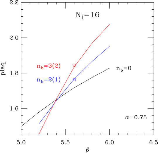
Figure 12: The matching of the plaquette for $N_{f}=16$ flavor. The individual data points are at $\beta=5.6$ on $16^{4}$ lattices after 2 and 3 levels of blocking. They are compared to the 1 and 2 times blocked values as measured on the $8^{4}$ lattices (solid lines). The matching values $\Delta\beta\approx 0$ indicate a nearly marginal flow. Note that the plaquette increases with $n_{b}$ implying that the RG flow is to an IRFP and not the $\beta=0$ trivial FP.

Just like in the $N_{f}=4$ case the mass dependence of the measured operators is weak for small $m$. Figure 11 shows the plaquette blocked 1 and 2 times on the $8^{4}$ configurations at $\beta=5.8$ at different masses. The solid lines are simple spline extrapolations. Within errors there is no mass dependence up to about $m\leq 0.05$ for the plaquette. Other observables are similar, so for the MCRG matching the $m=0.01-0.02$ data set can be considered critical in the mass.

Figure 12 is the analogue of Figures 2 and 8, showing the matching of the plaquette. The data points are at $\beta=5.6$ on $16^{4}$ lattices after 2 and 3 levels of blocking. They are compared to the 1 and 2 times blocked values as measured on the $8^{4}$ lattices. The block transformation is with parameter $\alpha=0.78$, optimal for $\beta=5.6$ and matching is consistent for both blocking levels with $\Delta\beta=0$.

From the matching value alone it is not possible to distinguish a marginally relevant flow (like at the GFP) from an almost marginal irrelevant flow (expected at the IRFP). Comparing Figure 12 to the $N_{f}=4$ or pure gauge Figures 2 and 8 reveals an important difference. When the flow is governed by the GFP the flow lines follow the RT towards the trivial $\beta=0$ FP. In the $n_{b}\to\infty$ limit all expectation values vanish. In Figures 2 and 8 the plaquette indeed decreases with increasing blocking levels. On the other hand when the flow lines approach an IRFP all expectation values take the value at the FP. The plaquette in Figure 12 increases with increasing blocking steps for $\beta\geq 5.4$, indicating that the flow lines are not running towards the $\beta=0$ FP. Eventually all expectation values should become independent of the blocking steps and $\beta$. This trend is not obvious from the figure for two main reasons. The first is that finite volume effects are considerable on $2^{4}$ lattices, the second that with only 2 or 3 blocking steps one approaches the FP only if the RG transformation is optimized. Nevertheless the fact that with optimal blocking the blocked operators increase with $n_{b}$ already signals that the flow runs toward an IRFP.

Other operators show similar behavior at $\beta\geq 5.6$ but the results are quite different at stronger gauge couplings. Figure 12 shows that the blocked plaquette values cross around $\beta=5.4$ and they decreases with $n_{b}$ for $\beta<5.4$. The location of the crossing depends on the blocking parameter but for the $N_{f}=16$ flavor model it never drops below $\beta=5.4$. It appears that the flow is running towards the $\beta=0$ FP when $\beta<5.4$ and to the IRFP when $\beta>5.4$.

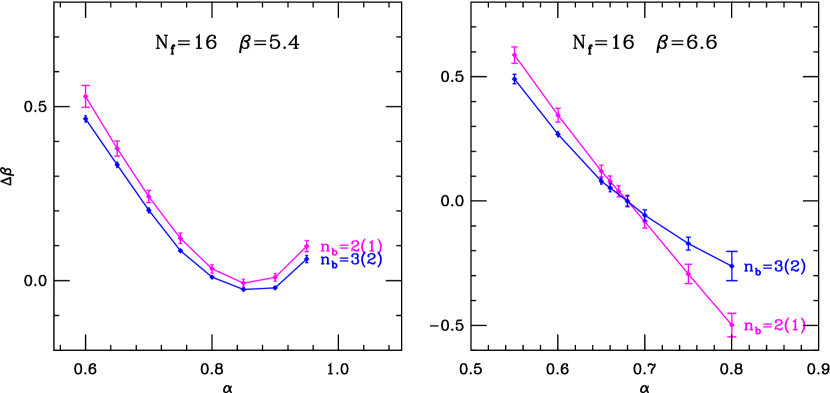
Figure 13: Matching at $\beta=5.4$ (left panel) and $\beta=6.6$ (right panel) from $16^{4}$ to $8^{4}$ lattices in the $N_{f}=16$ flavor theory.

$\beta_{16}$	$\alpha_{\rm{opt}}$	$s_{b}(s=2)$
5.4		none
5.6	0.78	0.00(3)
5.8	0.78	-0.12(4)
6.2	0.66	0.09(5)
6.6	0.67	-0.02(4)

Table 3: The parameters and MCRG results of the $N_{f}=16$ flavor simulations. The second column lists the optimal blocking parameter $\alpha$.

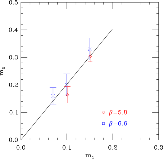
Figure 14: Matched $(m_{1},m_{2})$ pairs in the $N_{f}=16$ system. Red diamond: $\beta=5.8$, blue bursts: $\beta=6.6$. The linear fit predicts $y_{m}=1.02(7)$.

$\beta$	$\alpha_{\rm{opt}}$	$m_{1}$	$m_{2}$
5.8	0.75	0.10	0.17(3)
5.8	0.75	0.15	0.31(2)
6.6	0.68	0.07	0.16(3)
6.6	0.68	0.10	0.20(4)
6.6	0.68	0.15	0.33(4)

Table 4: Matched mass pairs in the $N_{f}=16$ system.

The 2-lattice matching is also different below and above $\beta=5.4$. Figure 13 shows $\Delta\beta$ as the function of the blocking parameter $\alpha$ for $\beta=5.4$ and $\beta=6.6$. This figure is the analogue of Figure 4. As the left panel of Figure 13 shows the $n_{b}=2(1)$ and 3(2) blocking levels get close but do not actually converge at $\beta=5.4$, there is no consistent matching. The situation is similar, even more enhanced, at stronger couplings. I have not observed this kind of behavior either with $N_{f}=0$ or 4, though I had simulations at even stronger couplings there. While it is possible that higher blocking levels would predict matching and the expectation values eventually approach their FP value, it is more likely that we see the effect of a nearby bulk transition and the strong coupling confining region beyond it. Apparently $\beta\leq 5.4$ is not governed by the IRFP. The situation is entirely different at $\beta=6.6$ where predictions from the two different blocking levels converge around $\alpha=0.675$ predicting $\Delta\beta=-0.022(44)$ (right panel of Figure 13). Results are similar at other $\beta>5.4$ couplings, as summarized in Table 3. The optimal block transformation predicts $\Delta\beta\approx 0$ for all coupling values, in agreement with the expectations, i.e. that the RG flows are governed by an almost marginal operator. Combining this with the observation that with optimal blocking parameter the expectation values of the blocked operators increase leads to the conclusion that the $\beta\in(5.6,6.6)$ coupling range in the massless limit is governed by an IRFP.

The mass is a relevant operator at this IRFP, therefore it should scale according to Eq. 8 under an $s=2$ RG transformation. One can calculate the exponent $y_{m}$ by identifying matched $(m_{1},m_{2})$ mass values. The gauge coupling is irrelevant, any $\beta$ in the attractive basin of the IRFP could be chosen for this. Since the gauge coupling is nearly marginal it is best to use the same coupling at both mass values. For matching one can use the same operators as before or add others that are more sensitive to the ferminons. I believe that direct fermionic observables would allow more precise matching at smaller quark masses, but as Figure 11 illustrates the gauge observables also work. In fact Figure 11 already shows a matched mass pair. At $\beta=5.8$ with $\alpha=0.75$ RG transformation the $m_{1}=0.15$ mass on the $16^{4}$ configurations match $m_{2}=0.318(6)$ on the $8^{4}$ configurations after 2(1) blocking steps, while the matching mass is $m_{2}=0.297(10)$ after 3(2) blocking steps. These values are for the plaquette but other observables give similar values, predicting $m_{2}=0.31(3)$ at the optimal $\alpha=0.75$ parameter. I have preliminary data at $\beta=5.8$ and 6.6 at a couple of mass values. The matching $(m_{1},m_{2})$ pairs are listed in Table 4. The fit according to Eq. 8 predicts $y_{m}=1.02(7)$ as shown in Figure 14 The scaling dimension of the mass is very close, within errors undistinguishable, form it engineering dimension. This is not unexpected as the IRFP is at weak coupling. In a recent publication $y_{m}=1.5$ was predicted for sextet fermions DeGrand (2009). It would be interesting to study the sextet model, or the $N_{f}=12$ model, where the $y_{m}$ might be significantly different from 1.

V Conclusion

Renormalization group methods have been designed to study the critical behavior of statistical systems. In this paper I have shown that they are equally suitable to study the renormalization group structure of quantum field theories. I have used a numerical Monte Carlo Renormalization Group method to calculate the step scaling function and critical exponent of SU(3) gauge theories with $N_{f}=0$, 4 and 16 flavors. I chose these fairly well understood systems as my goal was to test the method before using it in more relevant simulations. The paper is fairly pedagogical, explaining in detail the 2-lattice matching MCRG method.

In the $N_{f}=0$ case I demonstrated that the bare step scaling function predicted by the 2-lattice matching method is consistent with the more traditional Schrodinger functional results. It is also consistent with results obtained from the scaling of the $r_{0}$ parameter and the finite temperature phase transition even at strong gauge coupling, suggesting scaling, though not 2-loop perturbative scaling there.

The $N_{f}=4$ and 16 flavor simulations were done using nHYP smeared staggered fermions. I chose nHYP smearing because its highly improved taste symmetry. In the $N_{f}=4$ flavor case I briefly studied the finite temperature phase transition to develop a feel for the parameters of the model. I calculated the step scaling function at vanishing quark mass and showed that the 2-lattice method works equally well in the fermionic system.

The $N_{f}=16$ flavor model brings in new challenges as it is governed by an infrared fixed point at finite gauge coupling. At this IRFP the scaling dimension of the gauge coupling is small, it is an almost marginal operator. Accordingly the gauge coupling runs very slowly. The measured step scaling function is consistent with an almost marginal operator, but on its own it cannot predict if the gauge coupling is relevant or irrelevant. I argued that the evolution of blocked operators signal if the RG flow is towards an IRFP or to the $\beta=0$ trivial FP. For the $N_{f}=16$ model the flow clearly indicates an IRFP.

Finally I presented preliminary measurements for the scaling dimension of the mass. I found $y_{m}=1.02(7)$, undistinguishable from the free field exponent. This is not surprising for the $N_{f}=16$ theory.

VI Acknowledgment

I thank T. DeGrand and J. Kuti for discussions and T. DeGrand for his help with modifying the staggered nHYP code for many fermions. This research was partially supported by the US Dept. of Energy.

References

- Swendsen (1979) R. H. Swendsen, Phys. Rev. Lett. 42, 859 (1979).
- Swendsen (1981) R. H. Swendsen, Phys. Rev. Lett. 47, 1775 (1981).
- Swendsen (1984) R. H. Swendsen, Phys. Rev. Lett. 52, 2321 (1984).
- Hasenfratz et al. (1984a) A. Hasenfratz, P. Hasenfratz, U. M. Heller, and F. Karsch, Phys. Lett. B143, 193 (1984a).
- Hasenfratz et al. (1984b) A. Hasenfratz, P. Hasenfratz, U. M. Heller, and F. Karsch, Phys. Lett. B140, 76 (1984b).
- Bowler et al. (1985) K. C. Bowler et al., Nucl. Phys. B257, 155 (1985).
- Hasenfratz (1984) P. Hasenfratz, Lectures given at Int. School of Subnuclear Physics, Erice, Italy, Aug 5-15, 1984 (1984).
- Hasenfratz (1988) A. Hasenfratz, Phys. Lett. B201, 492 (1988).
- Decker et al. (1988) K. Decker, A. Hasenfratz, and P. Hasenfratz, Nucl. Phys. B295, 21 (1988).
- Gupta et al. (1984) R. Gupta, G. Guralnik, A. Patel, T. Warnock, and C. Zemach, Phys. Rev. Lett. 53, 1721 (1984).
- Patel and Gupta (1985) A. Patel and R. Gupta, Nucl. Phys. B251, 789 (1985).
- Appelquist et al. (2008) T. Appelquist, G. T. Fleming, and E. T. Neil, Phys. Rev. Lett. 100, 171607 (2008), eprint 0712.0609.
- Shamir et al. (2008) Y. Shamir, B. Svetitsky, and T. DeGrand, Phys. Rev. D78, 031502 (2008), eprint 0803.1707.
- Deuzeman et al. (2008) A. Deuzeman, M. P. Lombardo, and E. Pallante, Phys. Lett. B670, 41 (2008), eprint 0804.2905.
- Catterall et al. (2008) S. Catterall, J. Giedt, F. Sannino, and J. Schneible, JHEP 11, 009 (2008), eprint 0807.0792.
- Fodor et al. (2008a) Z. Fodor, K. Holland, J. Kuti, D. Nogradi, and C. Schroeder (2008a), eprint 0809.4888.
- Fodor et al. (2008b) Z. Fodor, K. Holland, J. Kuti, D. Nogradi, and C. Schroeder (2008b), eprint 0809.4890.
- Appelquist et al. (2009) T. Appelquist, G. T. Fleming, and E. T. Neil (2009), eprint 0901.3766.
- Hietanen et al. (2009a) A. J. Hietanen, K. Rummukainen, and K. Tuominen (2009a), eprint 0904.0864.
- Catterall and Sannino (2007) S. Catterall and F. Sannino, Phys. Rev. D76, 034504 (2007), eprint 0705.1664.
- Del Debbio et al. (2008a) L. Del Debbio, A. Patella, and C. Pica (2008a), eprint 0805.2058.
- Del Debbio et al. (2008b) L. Del Debbio, A. Patella, and C. Pica (2008b), eprint 0812.0570.
- DeGrand et al. (2009) T. DeGrand, Y. Shamir, and B. Svetitsky, Phys. Rev. D79, 034501 (2009), eprint 0812.1427.
- Hietanen et al. (2009b) A. J. Hietanen, J. Rantaharju, K. Rummukainen, and K. Tuominen, JHEP 05, 025 (2009b), eprint 0812.1467.
- Deuzeman et al. (2009) A. Deuzeman, M. P. Lombardo, and E. Pallante (2009), eprint 0904.4662.
- Banks and Zaks (1982) T. Banks and A. Zaks, Nucl. Phys. B196, 189 (1982).
- Hill and Simmons (2003) C. T. Hill and E. H. Simmons, Phys. Rept. 381, 235 (2003), eprint hep-ph/0203079.
- Sannino and Tuominen (2005) F. Sannino and K. Tuominen, Phys. Rev. D71, 051901 (2005), eprint hep-ph/0405209.
- Dietrich and Sannino (2007) D. D. Dietrich and F. Sannino, Phys. Rev. D75, 085018 (2007), eprint hep-ph/0611341.
- Fleming (2008) G. T. Fleming, PoS LATTICE2008, 021 (2008), eprint 0812.2035.
- DeGrand and Hasenfratz (2009) T. DeGrand and A. Hasenfratz (2009), eprint 0906.1976.
- Caswell (1974) W. E. Caswell, Phys. Rev. Lett. 33, 244 (1974).
- Luscher et al. (1993) M. Luscher, R. Sommer, U. Wolff, and P. Weisz, Nucl. Phys. B389, 247 (1993), eprint hep-lat/9207010.
- Luscher et al. (1994) M. Luscher, R. Sommer, P. Weisz, and U. Wolff, Nucl. Phys. B413, 481 (1994), eprint hep-lat/9309005.
- Capitani et al. (1999) S. Capitani, M. Luscher, R. Sommer, and H. Wittig (ALPHA), Nucl. Phys. B544, 669 (1999), eprint hep-lat/9810063.
- Gardi and Grunberg (1999) E. Gardi and G. Grunberg, JHEP 03, 024 (1999), eprint hep-th/9810192.
- DeGrand et al. (1995) T. A. DeGrand, A. Hasenfratz, P. Hasenfratz, and F. Niedermayer, Nucl. Phys. B454, 587 (1995), eprint hep-lat/9506030.
- Hasenfratz and Knechtli (2001a) A. Hasenfratz and F. Knechtli, Phys. Rev. D64, 034504 (2001a), eprint hep-lat/0103029.
- Sommer (1994) R. Sommer, Nucl. Phys. B411, 839 (1994), eprint hep-lat/9310022.
- Bilgici et al. (2009) E. Bilgici et al. (2009), eprint 0902.3768.
- Necco and Sommer (2002) S. Necco and R. Sommer, Nucl. Phys. B622, 328 (2002), eprint hep-lat/0108008.
- Boyd et al. (1996) G. Boyd et al., Nucl. Phys. B469, 419 (1996), eprint hep-lat/9602007.
- Hasenfratz et al. (2007) A. Hasenfratz, R. Hoffmann, and S. Schaefer, JHEP 05, 029 (2007), eprint hep-lat/0702028.
- Hasenfratz and Knechtli (2001b) A. Hasenfratz and F. Knechtli (2001b), eprint hep-lat/0105022.
- Bernard et al. (1996) C. W. Bernard et al., Phys. Rev. D54, 4585 (1996), eprint hep-lat/9605028.
- Heller (1998) U. M. Heller, Nucl. Phys. Proc. Suppl. 63, 248 (1998), eprint hep-lat/9709159.
- Damgaard et al. (1997) P. H. Damgaard, U. M. Heller, A. Krasnitz, and P. Olesen, Phys. Lett. B400, 169 (1997), eprint hep-lat/9701008.
- Iwasaki et al. (2004) Y. Iwasaki, K. Kanaya, S. Kaya, S. Sakai, and T. Yoshie, Phys. Rev. D69, 014507 (2004), eprint hep-lat/0309159.
- DeGrand (2009) T. DeGrand (2009), eprint 0906.4543.