Analysis of relative influence of nodes in directed networks

Abstract

Many complex networks are described by directed links; in such networks, a link represents, for example, the control of one node over the other node or unidirectional information flows. Some centrality measures are used to determine the relative importance of nodes specifically in directed networks. We analyze such a centrality measure called the influence. The influence represents the importance of nodes in various dynamics such as synchronization, evolutionary dynamics, random walk, and social dynamics. We analytically calculate the influence in various networks, including directed multipartite networks and a directed version of the Watts-Strogatz small-world network. The global properties of networks such as hierarchy and position of shortcuts, rather than local properties of the nodes, such as the degree, are shown to be the chief determinants of the influence of nodes in many cases. The developed method is also applicable to the calculation of the PageRank. We also numerically show that in a coupled oscillator system, the threshold for entrainment by a pacemaker is low when the pacemaker is placed on influential nodes. For a type of random network, the analytically derived threshold is approximately equal to the inverse of the influence. We numerically show that this relationship also holds true in a random scale-free network and a neural network.

I Introduction

Networks abound in various fields; a network is a collection of nodes and links, where a link connects a pair of nodes. Most real-world networks are not entirely regular or random and have prominent properties as modeled by, for example, small-world, scale-free, hierarchical, and modular networks reviews ; Boccaletti06 . In such networks, some nodes are considered to be more important than the others. Depending on the definition of importance, various centrality measures, which quantify the relative importance of different nodes, have been proposed. The most frequently used centrality measures are perhaps the degree (i.e., the number of links owned by a node) and the betweenness (i.e., the normalized number of shortest paths connecting any pair of nodes passing through the node in question) Boccaletti06 ; Freeman79 ; Wasserman94 . New centrality measures have also been proposed in the field of complex networks Noh04prl-Newman05soc-Estrada05-Latora07 ; Restrepo06prl .

Although many centrality measures are available, very few of these describe the importance of nodes in collective behavior of nodes on networks (see Restrepo06prl ). In a previous study, we proposed a centrality measure called the influence MKK09-1 . The influence of a node denotes its importance in different types of dynamics. It represents the amplitude of the response of a synchronized network when an input is given to a certain node Kori08 , the fixation probability for a newly introduced type (e.g., new information) at a node in voter-type evolutionary dynamics Masuda09njp , the stationary density of a simple random walk in continuous time Masuda09njp , the so-called reproductive value of a node Taylor90-Taylor96 , and the influence of a node in the DeGroot’s model of consensus formation Degroot74-Friedkin91 . It makes sense to consider the influence only in directed networks; in undirected networks, the influences of all the nodes take an identical value. In principle, the influence as a centrality measure is close to the PageRank, which was originally developed for ranking websites Brin98-Berkhin05 .

To assess the influence (and also the PageRank) in real complex networks, it is not sufficient to take into account the local property of the node, such as the degree. The global structure of networks such as the small-world property, modular structure, and self-similarity reviews ; Boccaletti06 generally affects the influence values.

In the present study, we analytically determine the influence of nodes in model networks such as weighted chain, directed multipartite networks with a hierarchical structure, and a directed version of the Watts-Strogatz small-world network Watts98 . For this purpose, we exploit the symmetry in networks and the relationship between the enumeration of directed spanning trees and the influence. We reveal the discrepancy between the actual influence and that predicted by the mean-field approximation (MA), which takes into account only the degree. In fact, the nodes that occupy globally important positions in terms of influence are generally different from those that are locally important. The globally important nodes govern the above-mentioned dynamics on networks. Finally, to demonstrate the application of the influence as a centrality measure, we analyze a system of coupled oscillators and show that nodes with large influence values entrain other nodes relatively easily, i.e., with a relatively small coupling strength.

II Influence

Consider a directed and weighted network having $N$ nodes. The weight of the directed link from node $i$ to node $j$ is denoted by $w_{ij}$. We set $w_{ij}=0$ when the link is absent. The influence of node $i$ is denoted by $v_{i}$. We define $v_{i}$ as the solution for the following set of $N$ linear equations:

$$v_{i}=\frac{\sum_{j=1}^{N}w_{ij}v_{j}}{k_{i}^{\rm in}},\quad(1\leq i\leq N),$$ (1)

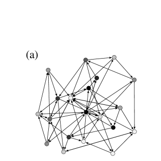
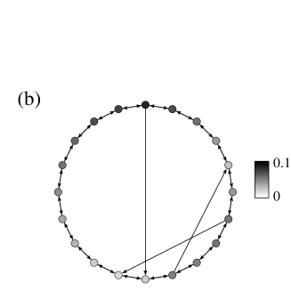
where $k_{i}^{\rm in}\equiv\sum_{j=1}^{N}w_{ji}$ is the indegree of node $i$, and the normalization is given by $\sum_{i=1}^{N}v_{i}=1$. When node $i$ has many outgoing links, $v_{i}$ can be large because there are many terms on the right-hand side of Eq. (1). When node $i$ has many incoming links, node $i$ is interpreted to be governed by many nodes. Then, $v_{i}$ can be small because of the divisive factor $k_{i}^{\rm in}$ in Eq. (1). The rationale for the definition given in Eq. (1) is that $v_{i}$ represents the importance of nodes in different types of dynamics on networks, as explained in Sec. I. Values of $v_{i}$ for two example networks are shown in Fig. 1.

Note that $v_{i}=1/N$ for any network with $k_{i}^{\rm in}=k_{i}^{\rm out}$ ($1\leq i\leq N$), where $k_{i}^{\rm out}\equiv\sum_{j=1}^{N}w_{ij}$ is the outdegree. The undirected network is included in this class of networks. Therefore, the influence has a nontrivial meaning only in directed networks. This situation also holds true in the case of the PageRank; in undirected networks, the PageRank is a linear function of the degree of node Brin98-Berkhin05 .

The MA of $v_{i}$ is given by

$$v_{i}=\frac{\sum_{j=1}^{N}w_{ij}v_{j}}{k_{i}^{\rm in}}\approx\frac{\sum_{j=1}^{N}w_{ij}\bar{v}}{k_{i}^{\rm in}}\propto\frac{k_{i}^{\rm out}}{k_{i}^{\rm in}},$$ (2)

where $\bar{v}\equiv\sum_{j=1}^{N}v_{j}/N=1/N$. In Secs. III and IV, we argue that Eq. (2) does not satisfactorily describe $v_{i}$ in certain practically important types of networks, including the Watts-Strogatz small-world network. For these networks, we calculate the exact $v_{i}$ by using different methods.

The value of $v_{i}$ can be associated with the number of directed spanning trees rooted at node $i$, as described below. Equation (1) implies that $v_{i}$ is the left eigenvector of the Laplacian matrix $L$, whose ($i,j$) element is equal to $L_{ii}=\sum_{j=1,j\neq i}^{N}w_{ji}$ and $L_{ij}=-w_{ji}$ ($i\neq j$). The corresponding eigenvalue is equal to 0; $\sum^{N}_{i=1}v_{i}L_{ij}=0$ ($1\leq j\leq N$). The $(i,j)$ cofactor of $L$ is given as

$$D\left(i,j\right)\equiv(-1)^{i+j}\det L\left(i,j\right),$$ (3)

where $L(i,j)$ is an $(N-1)\times(N-1)$ matrix obtained by deleting the $i$th row and the $j$th column of $L$. Because $\sum_{j=1}^{N}L_{ij}=0$ ($1\leq i\leq N$), $D\left(i,j\right)$ is independent of $j$. Therefore, considering the fact that $L$ has eigenvalue 0, we obtain

$$\sum_{i=1}^{N}D(i,i)L_{ij} =\sum_{i=1}^{N}D(i,j)L_{ij}$$

$$=\det L=0,\quad(1\leq j\leq N).$$ (4)

Equation (4) indicates that $\left[D\left(1,1\right),\ldots,D\left(N,N\right)\right]$ is the left eigenvector of $L$ with eigenvalue 0. Therefore, we obtain

$$v_{i}\propto D\left(i,i\right)=\det L\left(i,i\right).$$ (5)

According to the matrix tree theorem ref:biggs-ref:agaev , $\det L\left(i,i\right)$ is equal to the sum of the weights of all directed spanning trees of $G$ rooted at node $i$. The weight of a spanning tree is defined as the product of the weights of the $N-1$ links used in the spanning tree. Therefore, we can calculate $v_{i}$ by enumerating the spanning trees.

III Calculation of influence in some model networks

In this section, we analytically calculate the influence for several networks. Through these calculations, we show that the influence extracts the globally important nodes, which is beyond the scope of the MA: $k_{i}^{\rm out}/k_{i}^{\rm in}$. Such nodes are located upstream in the hierarchy that is defined by the directionality of the links or around the source of a valuable directed shortcut.

III.1 Weighted chain

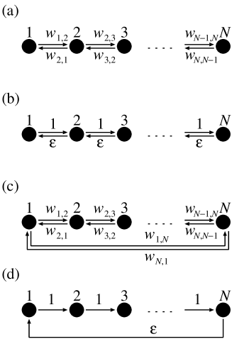
Consider a weighted chain of $N$ nodes, as shown in Fig. 2(a). There is a link from node $i$ to node $i+1$ with the weight $w_{i,i+1}>0$ for each $1\leq i\leq N-1$. There is a link from node $i$ to node $i-1$ with the weight $w_{i,i-i}>0$ for each $2\leq i\leq N$. Generally, $w_{i,i+1}$ is not equal to $w_{i+1,i}$. There are no other links. There is only one spanning tree rooted at each node $i$, which is represented by $1\leftarrow 2\leftarrow$ $\cdots\leftarrow i-1\leftarrow$ $i\to i+1\to$ $\cdots\to N-1\to N$, where the arrow denotes either a directed link or a directed path without confusion. Therefore,

$$v_{i}=\frac{w_{2,1}w_{3,2}\cdots,w_{i,i-1}w_{i,i+1}w_{i+1,i+2}\cdots w_{N-1,N}}{{\cal N}},$$ (6)

where the normalization constant is given by

$${\cal N}=\sum^{N}_{i=1}w_{2,1}w_{3,2}\cdots,w_{i,i-1}w_{i,i+1}w_{i+1,i+2}\cdots w_{N-1,N}.$$ (7)

Note that the position of the node, whether located in the middle or the periphery of the chain, does not affect the value of $v_{i}$.

Consider a special case where $w_{1,2}=w_{2,3}=\cdots=w_{N-1,N}=1$ and $w_{2,1}=w_{3,2}=\cdots=w_{N,N-1}=\epsilon$ [Fig. 2(b)]. For this network, we obtain

$$v_{i}=\frac{\epsilon^{i-1}(1-\epsilon)}{(1-\epsilon^{N})}.$$ (8)

When $\epsilon$ is small, node $i$ having a small $i$ is more influential. With the normalization constant neglected, the MA yields $k_{1}^{\rm out}/k_{1}^{\rm in}=1/\epsilon$, $k_{2}^{\rm out}/k_{2}^{\rm in}=\cdots=k_{N-1}^{\rm out}/k_{N-1}^{\rm in}=1$, and $k_{N}^{\rm out}/k_{N}^{\rm in}=\epsilon$. The MA is inconsistent with Eq. (8), except under the limit $\epsilon\to 0$, in which case $v_{1}\approx 1$, $v_{2},\ldots,v_{N}\approx 0$.

III.2 Weighted cycle

Consider a weighted cycle having $N$ nodes, as depicted in Fig. 2(c). The weighted cycle is constructed by adding two links $N\to 1$ and $1\to N$ with the weights $w_{N,1}$ and $w_{1,N}$, respectively, to the weighted chain.

In this network, there are $N$ spanning trees rooted at node $i$, i.e., $j\leftarrow j+1\leftarrow\cdots i-1\leftarrow i\to i+1\to\cdots\to j-1$, where $1\leq j\leq N$; nodes $N+1$ and 0 are identified with nodes 1 and $N$, respectively. Therefore, we obtain

$$v_{i} \propto w_{i,i+1}w_{i+1,i+2}\cdots w_{i-2,i-1}+w_{i,i-1}w_{i,i+1}\cdots w_{i-3,i-2}$$ (9)

$$+ w_{i-1,i-2}w_{i,i-1}w_{i,i+1}\cdots w_{i-4,i-3}+\cdots,$$

where $w_{N,N+1}\equiv w_{N,1}$ and $w_{1,0}\equiv w_{1,N}$.

In the weighted chain, only the weights of the descending links, i.e., $w_{j,j+1}$ for $j\geq i$ and $w_{j+1,j}$ for $j+1\leq i$, contribute to $v_{i}$. In contrast, in the weighted cycle, both $w_{j,j+1}$ and $w_{j+1,j}$ ($j,j+1\neq i$) contribute to $v_{i}$. Therefore, in the weighted cycle, the effect of each link weight on $v_{i}$ is more blurred than that in the case of the weighted chain. This property comes from the fact that node $i$ and node $j$ ($i\neq j$) are connected in two ways, i.e., clockwise and anticlockwise.

As a special case, consider a directed cycle in which $w_{2,1}=w_{3,2}=\cdots=w_{N,N-1}=w_{1,N}=0$, $w_{1,2}=w_{2,3}=\cdots=w_{N-1,N}=1$, and $w_{N,1}=\epsilon$ [Fig. 2(d)]. In this network, the values of the influence are equal to

$$v_{1} = \frac{1}{1+(N-1)\epsilon},$$ (10)

$$v_{2}=\cdots=v_{N} = \frac{\epsilon}{1+(N-1)\epsilon}.$$ (11)

The MA, which yields $k_{1}^{\rm out}/k_{1}^{\rm in}=1/\epsilon$, $k_{2}^{\rm out}/k_{2}^{\rm in}=\cdots=k_{N-1}^{\rm out}/k_{N-1}^{\rm in}=1$, and $k_{N}^{\rm out}/k_{N}^{\rm in}=\epsilon$, is inconsistent with Eq. (11) except when $\epsilon\to 0$.

III.3 Directed multipartite network

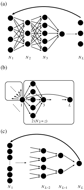
Consider the directed $L$-partite network, as schematically shown in Fig. 3(a). Layer $\ell$ ($1\leq\ell\leq L$) contains $N_{\ell}$ nodes. Each node in layer $\ell$ sends directed links to all the $N_{\ell+1}$ nodes in layer $\ell+1$, where layer $L+1$ is identified as layer 1. Because of symmetry, all nodes in layer $\ell$ have the same value of influence, denoted by $v_{\ell}$. From Eq. (1), we obtain

$$N_{\ell-1}v_{\ell}=N_{\ell+1}v_{\ell+1},\quad(1\leq\ell\leq L),$$ (12)

where $N_{0}\equiv N_{L}$. By combining Eq. (12) with the normalization condition $\sum^{L}_{\ell=1}N_{\ell}v_{\ell}=1$, we obtain

$$v_{\ell}=\frac{1}{N_{\ell-1}N_{\ell}\sum^{L}_{\ell^{\prime}=1}N_{\ell^{\prime}}^{-1}}.$$ (13)

III.3.1 Super-star

The super-star, which was introduced in Lieberman05 to study the fixation probability in networks, is a variant of the directed multipartite network. The super-star shown in Fig. 3(b) is generated as a superposition of a certain number of identical directed multipartite networks with $N_{1}=N_{3}=N_{4}=\cdots=N_{L}=1$ and $N_{2}=z$ ($\geq 1$). Each multipartite network is called a leave. The leaves are superposed such that they share a single node in layer 1. The indegree and outdegree of this node are equal to the number of leaves.

It can be easily shown that $v_{i}$ is independent of the number of leaves. Therefore, we consider the case of a single leave. Then, Eq. (13) yields

$$v_{1}=v_{4}=v_{5}=\cdots=v_{L} = \frac{z}{z(L-1)+1},$$ (14)

$$v_{2}=v_{3} = \frac{1}{z(L-1)+1}.$$ (15)

Surprisingly, the node in layer 1 does not have a particularly large influence value. Given $z\geq 2$, the nodes in the expanded layer (i.e., layer 2) and the node that receives convergent links from this layer (i.e., layer 3) have small influence values. These relationships are not predicted by the MA. The MA yields $k_{2}^{\rm out}/k_{2}^{\rm in}=k_{4}^{\rm out}/k_{4}^{\rm in}=k_{5}^{\rm out}/k_{5}^{\rm in}=\cdots=k_{N}^{\rm out}/k_{N}^{\rm in}=1$, $k_{1}^{\rm out}/k_{1}^{\rm in}=z$, and $k_{3}^{\rm out}/k_{3}^{\rm in}=1/z$; the actual $v_{1}$ and $v_{2}$ values are essentially smaller than the values predicted by the MA.

III.3.2 Funnel

The funnel, shown in Fig. 3(c), was introduced in Lieberman05 along with the super-star; it is also a directed multipartite network. The funnel has $N_{\ell}=z^{L-\ell}$ nodes in layer $\ell$ ($1\leq\ell\leq L$). Using Eq. (13), we obtain

$$v_{\ell}=\begin{cases}\displaystyle{\frac{z-1}{z^{L}-1}},\qquad&(\ell=1),\\[8.53581pt] \displaystyle{\frac{z-1}{z^{L}-1}\,z^{2\ell-L-2}},\qquad&(2\leq\ell\leq L).\end{cases}$$ (16)

The nodes in layer $L$ are most influential, and the node in layer 2 is least influential. The nodes in layer 1 are intermediately influential. For a large $z$, they are as influential as a node in layer $\approx L/2$. These relationships are not predicted by the MA, which yields the following results: $k_{1}^{\rm out}/k_{1}^{\rm in}=1$, $k_{2}^{\rm out}/k_{2}^{\rm in}=\cdots=k_{L-1}^{\rm out}/k_{L-1}^{\rm in}=z^{-1}$, and $k_{L}^{\rm out}/k_{L}^{\rm in}=z^{L-2}$.

III.4 Directionally biased random network

The networks considered in the previous sections have inherent global directionality due to the presence of asymmetrically weighted or unidirectional links from node to node or from layer to layer. The directionality of networks is a main cause for the deviation in the $v_{i}$ values from those predicted by the MA. To examine the effect of directionality in further detail, we study the directionally biased random network Kori06pre . To generate a network from this model, we prepare a strongly connected directed random graph with mean indegree and mean outdegree $z$ and specify a root node, which is placed in layer 1. The root node is the source of directed links to about $z$ nodes, which are placed in layer 2. We align all the nodes according to their distance from the root. Except in the layers near the last layer, the number of nodes in layer $\ell$ grows roughly as $z^{\ell-1}$. We set the weights of the forward links, i.e., links from layer $\ell$ to layer $\ell+1$, as unity. We set the weights of the backward links, i.e., links from layer $\ell$ to layer $\ell^{\prime}$, where $\ell>\ell^{\prime}$, as $\epsilon$. The weights of the parallel links, i.e., those connecting two nodes in the same layer, are arbitrary; they do not affect the value of $v_{i}$ in the following derivation. When $\epsilon=1$, the network is an unweighted directed random graph, if the weight of the parallel link is equal to unity at $\epsilon=1$. When $\epsilon=0$, the network is purely feedforward and no longer strongly connected. The feedforwardness is parametrized by $\epsilon$.

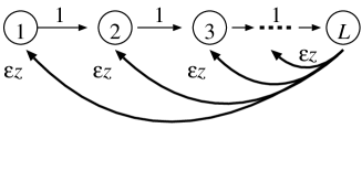
The directionally biased random network is approximated by using a modified tree as follows Kori06pre . We assume that each node has $z$ outgoing links and that each node except the root node has only one “parent” node, namely, the node in the previous layer from where it receives a feedforward link. Further assume that there are $L$ layers and that layer $\ell$ ($1\leq\ell\leq L$) has $z^{\ell-1}$ nodes. The number of nodes is equal to $(z^{L}-1)/(z-1)$. At this point, the constructed network is a tree. Then, we add backward links with weight $\epsilon$ to this tree. When $z$ is large, most backward links in the original network originate from layer $L$, because layer $L$ has a majority of nodes. Therefore, we assume that, in the approximated network, the backward links with weight $\epsilon$ originate only from the nodes in layer $L$. This approximation is accurate when $z$ is sufficiently large. The other links in the approximated network have the weight of unity. For a sufficiently large $z$, all nodes in the same layer have almost the same connectivity pattern. In terms of incoming links, a node receives approximately one forward link from the previous layer and $z$ backward links from layer $L$. The approximated network is schematically shown in Fig. 4. On an average, each node in layer $L$ is the source of an directed link to each node with an effective weight $\epsilon^{\prime}$. Because $k_{i}^{\rm out}=\epsilon z$ for a node in layer $L$ is approximated by $\epsilon^{\prime}(z^{L}-1)/(z-1)\approx\epsilon^{\prime}z^{L-1}$, we obtain $\epsilon^{\prime}\approx\epsilon z^{-L+2}$.

The influence of a node in layer $\ell$, denoted by $v_{\ell}$, satisfies the following relationships:

$$z^{L-1}\epsilon^{\prime}v_{1} = zv_{2},$$ (17)

$$(z^{L-1}\epsilon^{\prime}+1)v_{\ell} = zv_{\ell+1},\quad(2\leq\ell\leq L-1).$$ (18)

On substituting $\epsilon^{\prime}\approx\epsilon z^{-L+2}$ in Eq. (18) and considering the normalization given by

$$\sum_{\ell=1}^{L}z^{\ell-1}v_{\ell}=1,$$ (19)

we obtain

$$v_{\ell}\approx\begin{cases}\displaystyle{\left(\epsilon z+1\right)^{-L+1}},\qquad&(\ell=1),\\[8.53581pt] \displaystyle{\left(\epsilon z+1\right)^{-L+\ell-1}z^{-\ell+2}\epsilon},\qquad&(2\leq\ell\leq L).\end{cases}$$ (20)

For a small $\epsilon$, the network is close to feedforward, and $v_{1}$ is relatively large; $v_{\ell}$ varies as $v_{\ell}\propto\left(\epsilon+z^{-1}\right)^{\ell}$. When $z$ is sufficiently large, we obtain $v_{\ell}\propto\epsilon^{\ell}$, which coincides with the results obtained for the network shown in Fig. 2(b) (Sec. III.1).

To test our theory, we generate a directionally biased random network with $N=5000$ and $z=10$. For $\epsilon=0.5$, the values of $v_{i}$ of all the nodes are plotted against the values obtained from the MA in Fig. 5(a). Although the values obtained from the MA are strongly correlated with $v_{i}$, there is some variation in $v_{i}$ for a fixed $k_{i}^{\rm out}/k_{i}^{\rm in}$. The average and the standard deviation of $v_{i}$ in each layer are plotted by the circles and the corresponding error bars, respectively, in Fig. 5(b). The influence of a node decreases exponentially with $\ell$ as predicted by Eq. (20) [Eq. (20) for $\ell\geq 2$ is represented by the line in Fig. 5(b)]. The average and the standard deviation of $v_{i}$ obtained by the MA are plotted by the squares and the corresponding error bars, respectively. The values obtained from the MA are scaled by a multiplicative factor $C$, where $C$ is selected such that $v_{i}=Ck_{i}^{\rm out}/k_{i}^{\rm in}$ for the root node (i.e., $\ell=1$). Figure 5(b) shows that $k_{i}^{\rm out}/k_{i}^{\rm in}$ is generally small for node $i$ in a downstream layer. However, the decrease in $v_{i}$ with $\ell$ is much more than that in $k_{i}^{\rm out}/k_{i}^{\rm in}$. The hierarchical nature of the network is revealed by the $v_{i}$ values and not satisfactorily by the local degree. The results for $\epsilon=0.1$ shown in Figs. 5(c) and 5(d) provide further evidence for our claim.

III.5 Small-world networks

In this section, we analyze the influence in the directed unweighted small-world network model, which is a variant of the Watts-Strogatz model Watts98 . To generate a network, we start with an undirected cycle of $N$ nodes, in which each node is connected to its immediate neighbor on both sides. At this stage, $k_{i}^{\rm in}=k_{i}^{\rm out}=2$ is satisfied for all $i$. Then, we add a directed shortcut to the network, as schematically shown in Fig. 6(a). The source and the target of the shortcut are denoted by nodes $s$ and $t$, respectively. The distance between node $s$ and node $t$ along the cycle is assumed to be $\min(N_{1},N_{2})$, where $N_{2}\equiv N-N_{1}$.

We enumerate the number of directed spanning trees rooted at node $r$, which is $\overline{N}$ nodes away from node $s$ along the cycle, where $0\leq\overline{N}\leq\max(N_{1},N_{2})$. There are $N$ spanning trees that do not use the shortcut, as derived in Sec. III.2. Any spanning tree that uses the shortcut includes the directed path $r\to\cdots\to s$, which contains $\overline{N}+1$ nodes. The choice of the other links is arbitrary with the restriction that a spanning tree must be formed. The $N_{1}-\overline{N}-1$ nodes between node $r$ and node $t$ in Fig. 6(a) are reached from node $r$ or node $t$ by a directed path along the cycle. There are $N_{1}-\overline{N}$ choices regarding the formation of this part of the spanning tree. The $N_{2}-1$ nodes between node $s$ and node $t$ are reached from node $s$ or node $t$ by a directed path along the cycle. There are $N_{2}$ choices regarding the formation of this part of the spanning tree. In sum, there are $N+(N_{1}-\overline{N})N_{2}$ spanning trees rooted at $v$. Therefore, the influence of $v$ is large (small) for the $v$ that is close to the source (target) of the shortcut. In the region on the cycle where no source or target of a shortcut is located, the influence of a node changes linearly with the distance between the source of the shortcut and the node, because $N+(N_{1}-\overline{N})N_{2}\propto-\overline{N}$. We call such a region, including the two border points, the segment.

Next, we consider small-world networks with two directed shortcuts. There are three qualitatively different possible arrangements of the shortcuts, as shown in Figs. 6(b)–6(d). The lengths of the four segments are denoted by $N_{1}$, $N_{2}$, $N_{3}$, and $N_{4}$, such that $N_{1}+N_{2}+N_{3}+N_{4}=N$.

In the network shown in Fig. 6(b), a node is located at either of the three essentially different positions denoted by $a$, $b$, and $c$. We first enumerate spanning trees rooted at node $a$. The distance from node $a$ to the source of a shortcut, i.e., node $s$, is denoted by $\overline{N}$ ($0\leq\overline{N}\leq N_{1}$). There are $N$ spanning trees that do not use the shortcuts. There are $(N_{1}-\overline{N})(N_{2}+N_{3}+N_{4})$ spanning trees that use the shortcut $s\to t$ but not $s^{\prime}\to t^{\prime}$. There are $(N_{1}+N_{2}-\overline{N})N_{3}$ spanning trees that use the shortcut $s^{\prime}\to t^{\prime}$ but not $s\to t$. There are $(N_{1}-\overline{N})N_{2}N_{3}$ spanning trees that use both shortcuts, which can be explained as follows. The directed path $a\to s\to s^{\prime}$ is included in such a spanning tree. The $N_{1}-\overline{N}-1$ nodes between node $a$ and node $t$ are reached along the cycle from node $a$ or node $t$. The $N_{2}-1$ nodes between node $t$ and node $t^{\prime}$ are reached along the cycle from node $t$ or node $t^{\prime}$. The $N_{3}-1$ nodes between node $t^{\prime}$ and node $s^{\prime}$ are reached along the cycle from node $t^{\prime}$ or node $s^{\prime}$. In sum, the number of spanning trees rooted at node $a$ is equal to

$$N+(N_{1}-\overline{N})(N_{2}+N_{3}+N_{4})+(N_{1}+N_{2}-\overline{N})N_{3}+(N_{1}-\overline{N})N_{2}N_{3},$$ (21)

which is proportional to the influence of node $a$. If $N$ is sufficiently large and the two shortcuts are randomly placed, the last term in Eq. (21) is of the highest order because $N_{i}=O(N)$ ($1\leq i\leq 4$). As in the case of the network with one shortcut, the influence changes linearly within one segment.

Similarly, the number of spanning trees rooted at node $b$ is equal to

$$N+N_{1}(N_{2}+N_{3}+N_{4}-\overline{N})+(N_{1}+N_{2}+\overline{N})N_{3}+N_{1}N_{2}N_{3},$$ (22)

where $\overline{N}$ ($0\leq\overline{N}\leq N_{4}$) is the distance from node $b$ to node $s$ along the cycle. The number of spanning trees rooted at node $c$ is equal to

$$N+(N_{2}-\overline{N})N_{3}+N_{1}\overline{N},$$ (23)

where $\overline{N}$ ($0\leq\overline{N}\leq N_{2}$) is the distance from node $c$ to node $t$ along the cycle. Owing to the absence of a third-order term in Eq. (23), the influence values of the nodes located on the segment between the two targets of the shortcuts are very small.

The quantities given in Eqs. (21)–(23) are linear in $\overline{N}$. Therefore, the influence changes linearly within each segment. This is true for the other two types of arrangements of shortcuts shown in Figs. 6(c) and 6(d).

This linear relationship also holds true in the case of more than two shortcuts. To show this, we consider a general directed small-world network and focus on a segment on the cycle, which is schematically shown in Fig. 6(e). Without loss of generality, we assume that a node $v$ in the segment is located $\overline{N}$ and $N_{1}-\overline{N}$ nodes away from the two border points of the segment. We distinguish three types of spanning trees rooted at node $r$. First, some spanning trees include both $r\to\cdots\to 1$ and $r\to\cdots\to 2$. We denote the number of such spanning trees by $S_{1}$. Second, some spanning trees include $r\to\cdots\to 1$ and not $r\to\cdots\to 2$. For these spanning trees, node $2$ is reached via a path $r\to 1\to\cdots\to 2$. To enumerate such spanning trees, denote by $S_{2}$ the number of directed trees that span the network excluding the nodes in the segment between node $r$ and node $2$. Third, the other spanning trees include $r\to\cdots\to 2$ and not $r\to\cdots\to 1$. Denote by $S_{3}$ the number of directed trees that span the network excluding the nodes in the segment between node $r$ and node $1$. The number of spanning trees rooted at node $r$ is equal to

$$S_{1}+S_{2}(N_{1}-\overline{N})+S_{3}\overline{N}.$$

Therefore, the influence of node $r$ changes linearly with $\overline{N}$ ($0\leq\overline{N}\leq N_{1}$).

The thick line in Fig. 7(a) indicates the numerically obtained values of $v_{i}$ for a small-world network with three shortcuts. We set $N=5000$. The nodes are aligned according to their position in the cycle. In accordance with the theoretical prediction, $v_{i}$ changes linearly with $i$ within each segment. $v_{i}$ is very small for $1250\leq i\leq 1666$, because these nodes are between two targets of shortcuts.

In theory, it is assumed that each node is initially connected to only its nearest neighbors on the cycle (i.e., $k_{i}^{\rm in}=k_{i}^{\rm out}=2$). However, values of $v_{i}$ are almost the same if the underlying cycle has $k_{i}^{\rm in}=k_{i}^{\rm out}=4$ (i.e., each node is connected to two neighbors on each side) or $k_{i}^{\rm in}=k_{i}^{\rm out}=6$. The results for $k_{i}^{\rm in}=k_{i}^{\rm out}=4$ and those for $k_{i}^{\rm in}=k_{i}^{\rm out}=6$ are indicated by the medium and thin lines, respectively, in Fig. 7(a). The three lines are observed to almost overlap with each other.

To examine the effect of shortcuts in more general small-world networks, we generate a small-world network by rewiring many links Watts98 . We place $N=5000$ nodes on a cycle and connect a node to its five immediate neighbors on each side, such that $k_{i}^{\rm in}=k_{i}^{\rm out}=10$. Then, out of 50000 directed links, we rewire 500 randomly selected ones to create directed shortcuts. The sources and targets of shortcuts are chosen randomly from the network with the restriction that self loops and multiple links must be avoided. Because of rewiring, the mean degree $\left<k\right>=10$.

As shown in Fig. 7(b), the MA strongly disagrees with the observed $v_{i}$ Masuda09njp . The values of $v_{i}$ are plotted against the circular positions of the nodes in Fig. 7(c). $v_{i}$ changes gradually along the cycle, which is consistent with our analytical results. The peaks and troughs in Fig. 7(c) correspond to the sources and targets of the shortcuts, respectively. For a node near a source (target), $v_{i}$ is large (small), whereas the MA estimate $\propto k_{i}^{\rm out}/k_{i}^{\rm in}$ is not as affected by the position of the shortcuts as $v_{i}$. The relationship between $v_{i}/(k_{i}^{\rm out}/k_{i}^{\rm in})$ and $v_{i}$ is shown in Fig. 7(d). The MA is exact along the horizontal line, i.e., $v_{i}=(k_{i}^{\rm out}/k_{i}^{\rm in})/(\sum_{j=1}^{N}k_{j}^{\rm out}/k_{j}^{\rm in})$. Nodes with large (small) $v_{i}$ tend to be located near sources (targets) of shortcuts. For such nodes, $v_{i}$ is usually larger (smaller) than the value obtained by the MA.

IV Entrainment of a network by a pacemaker

As an application of the influence as a centrality measure, we examine a system of coupled phase oscillators having a pacemaker Kori06pre ; Kori04prl . Consider a dynamical system of phase oscillators given by

$$\dot{\phi}_{i}=\omega_{i}+\frac{\kappa}{\left<k\right>}\sum_{j=1}^{N}w_{ji}\sin\left(\phi_{j}-\phi_{i}\right),\qquad(1\leq i\leq N),$$ (24)

where the mean degree $\left<k\right>=\sum_{i^{\prime},j^{\prime}=1}^{N}w_{i^{\prime}j^{\prime}}/N$ provides the normalization for the coupling strength $\kappa$. The phase and the intrinsic frequency of the $i$th oscillator are denoted by $\phi_{i}\in[0,2\pi)$ and $\omega_{i}$, respectively. We assume a pacemaker, i.e., an oscillator that is not influenced by the other oscillators, in the network. Equation (24) emulates a pacemaker system, where the pacemaker is placed at node $i_{0}$, if we force $w_{ji_{0}}=0$ ($1\leq j\leq N$). We examine the possibility of the pacemaker to entrain the other oscillators into its own intrinsic rhythm. For this, we assume that $\omega_{i}=\omega$ ($i\neq i_{0}$) is identical for the $N-1$ oscillators and that $\omega_{i_{0}}$ takes a different value. By redefining $\phi_{i}-\omega t$ as the new $\phi_{i}$ and rescaling time, we set $\omega_{i_{0}}=1$ and $\omega_{i}=0$ ($i\neq i_{0}$) without loss of generality.

Depending on the network and the position of the pacemaker, there exists a critical threshold $\kappa_{\rm cr}$ such that the entrainment is realized for $\kappa>\kappa_{\rm cr}$ Kori04prl ; Kori06pre . When entrained, the actual frequency of all oscillators becomes exactly the same as that of the pacemaker, i.e., $\omega_{i_{0}}=1$. Thus, the condition for the entrainment is given by

$$\dot{\phi}_{i}=\frac{\kappa}{\left<k\right>}\sum_{j=1}^{N}w_{ji}\sin\left(\phi_{j}-\phi_{i}\right)=1,\qquad(1\leq i\leq N,i\neq i_{0}).$$ (25)

In general, entrainment Kori06pre ; Masuda07jcn and synchrony syn-forward-pre are easily realized for feedforward networks. Because of the intuitive meaning of the influence, $\kappa_{\rm cr}$ may be small if $v_{i_{0}}$ is large. We analytically show this for the directionally biased random network with a sufficiently large $z$. In the directionally biased random network, a node in layer $\ell$ receives a forward link with weight unity from layer $\ell-1$. Although a forward link is absent for a node in layer 1, this factor is negligible because layer 1 contains only one node. Most backward links with weight $\epsilon$ to a node in layer $\ell$, where $\ell\leq L-1$, originate from layer $L$, as discussed in Sec. III.4. The number of parallel links is smaller than that of backward links. We assume that the weight of the parallel link, which was assumed to be arbitrary in Sec. III.4, is equal to $\epsilon$, such that all the incoming links to a node in layer $L$, except one forward link, also have weight $\epsilon$. Under this condition, we approximate $\left<k\right>\approx 1+\epsilon z$.

Denote by $\kappa_{\rm cr}^{(\ell)}$ the typical critical coupling strength when the pacemaker is located at a node in layer $\ell$ in a directionally biased random network. First, we consider the case in which node $i_{0}$ coincides with the root node in the directionally biased random network, i.e., $\ell=1$. This case was analyzed in our previous studies Kori06pre ; Kori04prl . In the entrained state, the phase difference between the oscillators in the same layer is small, and the phases of the oscillators in layers with small $\ell$ are more advanced. Therefore, we assume that the phases of all the oscillators in the same layer are identical. We set the difference between the phase of the oscillator in layer $\ell$ and that in layer $\ell+1$ to $\varDelta\phi_{\ell}$. The entrainment occurs if and only if $\varDelta\phi_{1}$, $\ldots$, $\varDelta\phi_{L-1}$ stay constant in a long run. We obtain Kori06pre ; Kori04prl

$$\varDelta\phi_{\ell}=\frac{\left(1+\epsilon z\right)^{L-\ell}}{\kappa},\qquad(1\leq\ell\leq L-1).$$ (26)

By applying the threshold condition $\varDelta\phi_{1}=1$, we obtain

$$\kappa_{\rm cr}^{(1)}=\left(1+\epsilon z\right)^{L-1}.$$ (27)

Next, we consider the case in which node $i_{0}$ is located in layer $L$. We expect $\kappa_{\rm cr}^{(L)}$ to be large because the pacemaker is located downstream of the network. To analyze this case, we redraw the network as a directionally biased random network, such that node $i_{0}$ is located at the root. Then, statistically, the network is the same as the original directionally biased random network in terms of the positions of the nodes and the links. However, the effective link weight in the redrawn network is equal to $\epsilon$, because most links in the original network are backward links with weight $\epsilon$. By assuming that all links in the redrawn network have weight $\epsilon$, the result for unweighted directed random graph Kori06pre ; Kori04prl translates into

$$\varDelta\phi_{\bar{\ell}}=\frac{(1+\epsilon z)\left(1+z\right)^{L-\bar{\ell}-1}}{\kappa\epsilon},\qquad(1\leq\bar{\ell}\leq L-1),$$ (28)

where $\bar{\ell}$ is the layer number in the redrawn network. Analogous to the derivation of Eq. (27) from Eq. (26), from Eq. (28), we derive

$$\kappa_{\rm cr}^{(L)}=\frac{(1+\epsilon z)\left(1+z\right)^{L-2}}{\epsilon}.$$ (29)

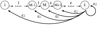
When node $i_{0}$ is located in the $(L-M+1)$th layer $(2\leq M\leq L-1)$ in the original network, we redraw the network in a similar manner, such that node $i_{0}$ is located at the root. The redrawn network is schematically shown in Fig. 8. For this network, we obtain

$$\varDelta\phi_{\bar{\ell}}=\begin{cases}\frac{\left(1+z\right)^{L-M}\left(1+\epsilon z\right)^{M-\bar{\ell}}}{\kappa},\qquad&(1\leq\bar{\ell}\leq M-1),\\ \frac{(1+\epsilon z)\left(1+z\right)^{L-\bar{\ell}-1}}{\kappa\epsilon},\qquad&(M\leq\bar{\ell}\leq L-1),\end{cases}$$ (30)

which yields

$$\kappa_{\rm cr}^{(L-M+1)}=\left(1+\epsilon z\right)^{M-1}\left(1+z\right)^{L-M}.$$ (31)

From Eqs. (27), (29), and (31), we obtain

$$\kappa_{\rm cr}^{(\ell)}=\begin{cases}\left(1+\epsilon z\right)^{L-\ell}\left(1+z\right)^{\ell-1},\qquad&(1\leq\ell\leq L-1),\\ \frac{\left(1+\epsilon z\right)\left(1+z\right)^{L-2}}{\epsilon},\qquad&(\ell=L).\end{cases}$$ (32)

Under the condition $\epsilon z\gg 1$, Eq. (32) gives

$$\kappa_{\rm cr}^{(\ell)}\approx\epsilon^{L-\ell}\,z^{L-1},\qquad(1\leq\ell\leq L).$$ (33)

Moreover, Eq. (20) yields

$$v_{\ell}\approx\epsilon^{-L+\ell}\,z^{-L+1},\qquad(1\leq\ell\leq L).$$ (34)

Therefore, we obtain

$$\kappa_{\rm cr}^{(\ell)}\approx\frac{1}{v_{\ell}},\qquad(1\leq\ell\leq L).$$ (35)

Equation (35) shows that the pacemaker located at an influential node can easily realize the entrainment. We validate this prediction by direct numerical simulations of the pacemaker system on a directionally biased random network with $N=200$, $z=10$, and $\epsilon=0.1$. To judge whether the entrainment has been realized for a value of $\kappa$, we measure the ratio of $\sum_{i=1,i\neq i_{0}}^{N}\left[\phi_{i}\left(t=T\right)-\phi_{i}\left(t=0.8T\right)\right]\big{/}\left(N-1\right)$ to $\phi_{i_{0}}(t=T)-\phi_{i_{0}}(t=0.8T)$, where $T$ is the duration of a run. The first 80% of a run is discarded as transient. The ratio represents the average phase shift of the oscillators, other than the pacemaker, relative to that of the pacemaker. If this value is more than 0.99, we consider the entrainment to be achieved. Because the transient is shorter for larger $\kappa$, we set $T=5\times 10^{5}/\kappa$.

The values of $\kappa_{\rm cr}$ when the pacemaker is located at different nodes are plotted against $v_{i}$ in Fig. 9(a). The line in the figure represents $\kappa_{\rm cr}=v_{i}^{-1}$, i.e., Eq. (35). The numerically obtained $\kappa_{\rm cr}$ roughly matches the theoretical one although the condition $\epsilon z\gg 1$ is violated. The same values of $\kappa_{\rm cr}$ are plotted against the MA estimate $v_{i}\approx(k_{i}^{\rm out}/k_{i}^{\rm in})/\sum_{j=1}^{N}(k_{j}^{\rm out}/k_{j}^{\rm in})$ in Fig. 9(b). We find a larger spread of data in this plot as compared to that in Fig. 9(a); $v_{i}$ predicts $\kappa_{\rm cr}$ more accurately than the MA.

Next, we set the weight of the parallel link to unity, as done in Kori06pre . The values of $\kappa_{\rm cr}$ for this version of the directionally biased random network are shown in Figs. 9(c) and 9(d). The results are qualitatively the same as those shown in Figs. 9(a) and 9(b). The dependence of $\kappa_{\rm cr}$ on $v_{i}$ is weak in the new network [Fig. 9(c)] as compared to the previous network [Fig. 9(a)] mainly for the following reason. Because of the difference in the weights of parallel links, $\left<k\right>$ in the new network is larger than that in the previous network. Then, $\kappa_{\rm cr}^{(L)}$ is smaller for the new network, since it is inversely proportional to the effective link weight. We expect that $\kappa_{\rm cr}$ for nodes in intermediate layers can also be explained using the same approach.

The result $\kappa_{\rm cr}\approx v_{i}^{-1}$ is derived for the directionally biased random network. Although it is not guaranteed that this relationship holds true in other types of networks, we test the applicability of the relation $\kappa_{\rm cr}\approx v_{i}^{-1}$ in a scale-free network and a neural network.

We generate a directed scale-free network using the configuration model reviews . The degree distributions are independently given for $k_{i}^{\rm in}$ and $k_{i}^{\rm out}$ by $p(k^{\rm in})\propto k^{-\gamma_{\rm in}}$ and $p(k^{\rm out})\propto k^{-\gamma_{\rm out}}$, respectively. We set $\gamma_{\rm in}=\gamma_{\rm out}=2.5$ and $N=200$. The minimum degree is set to 3. The duration of a run and the length of the traisient are equal to those in the case of the directionally biased random networks. The values of $\kappa_{\rm cr}$ are plotted against $v_{i}$ and the MA in Figs. 9(e) and 9(f), respectively. The relation $\kappa_{\rm cr}\approx v_{i}^{-1}$ fits the data reasonably well, even though the scale-free network is not a directionally biased random network. In contrast, $k_{i}^{\rm out}/k_{i}^{\rm in}$ poorly predicts $\kappa_{\rm cr}$, as shown in Fig. 9(f).

We next examine the C. elegans neural network Chen06pnas ; wormatlas based on chemical synapses, which serve as directed links. The network has the largest strongly connected component with $N=237$ nodes. The number of synapses from neuron $i$ to neuron $j$ defines $w_{ij}$. We set $T=2.5\times 10^{7}/\kappa$ to appropriately exclude the transient. The values of $\kappa_{\rm cr}$ are plotted against $v_{i}$ and the MA in Figs. 9(g) and 9(h), respectively. The values of $\kappa_{\rm cr}$ exceeding $10^{7}$ are not plotted because direct numerical simulations need too much time. Similar to the case of scale-free networks, $v_{i}$ predicts $\kappa_{\rm cr}$ better than $k_{i}^{\rm out}/k_{i}^{\rm in}$ does.

V Conclusions

In this paper, we have analyzed the centrality measure called the influence in various networks. The influence extracts the magnitude with which a node controls or impacts the entire network along directed links. We have analytically shown that the source of the shortcut in a directed version of the Watts-Strogatz small-world network and the root node in hierarchical networks have large influence values. This is not accurately predicted if we approximate the influence of a node by its degree. Although by definition, the influence is based on local connectivity, the global structure of networks does affect the influence values. We also analyzed the effect of the location of a pacemaker on the capability of entrainment in a system of coupled phase oscillators. The pacemaker located at a node with a large influence value entrains the other oscillators relatively easily.

In the analysis of some model networks, including the Watts-Strogatz small-world network, we used the method based on the enumeration of directed spanning trees. This method can be applied to the estimation of the PageRank of nodes, because the PageRank can be mapped to the influence if we reverse links and rescale the link weight MKK09-1 ; Masuda09njp . Application of our results to other centrality measures for directed networks is warranted for future study.

Figure 1: Influence of nodes in networks having $N=20$. A dark node has a large value of $v_{i}$. (a) Directed network generated by the configuration model. The indegree and outdegree follow independent power-law distributions with the scaling exponent 2.5 and the minimum degree 2. (b) Directed Watts-Strogatz network with three shortcuts. See Secs. III.5 and IV for details of the network models. The networks are visualized by Pajek pajek .

Figure 2: Schematic of (a) weighted chain, (b) special case of weighted chain, (c) weighted cycle, and (d) special case of weighted cycle.

Figure 3: Schematic of (a) multipartite network, (b) super-star, and (c) funnel.

Figure 4: Schematic of directionally biased random network under tree approximation.

Figure 5: $v_{i}$ for a directionally biased random network with $N=5000$. We set [(a) and (b)] $\epsilon=0.5$ and [(c) and (d)] $\epsilon=0.1$. In (a) and (c), $v_{i}$ is plotted against the MA results. The lines represent the MA: $v_{i}=(k_{i}^{\rm out}/k_{i}^{\rm in})/\sum_{j=1}^{N}(k_{j}^{\rm out}/k_{j}^{\rm in})$. In (b) and (d), $v_{i}$ (circles) and rescaled $k_{i}^{\rm out}/k_{i}^{\rm in}$ (squares) averaged over all the nodes in each layer are plotted against layer number. The error bars indicate the standard deviation obtained from $v_{i}$ of all the nodes in the same layer.

Figure 6: Schematics of directed small-world network having (a) one shortcut, [(b)–(d)] two shortcuts, and (e) general number of shortcuts.

Figure 7: $v_{i}$ in directed small-world networks with $N=5000$. (a) Results for small-world network with three added shortcuts. The thick, medium, and thin lines correspond to the networks in which the mean degree of the underlying cycle is equal to 2, 4, and 6, respectively. (b, c, d) Results for directed small-world network with $\left<k\right>=10$ and 500 rewired shortcuts. In (a) and (c), $v_{i}$ is plotted against the position of the node in the underlying cycle. In (b), $v_{i}$ is plotted against $(k_{i}^{\rm out}/k_{i}^{\rm in})/\sum_{j=1}^{N}(k_{j}^{\rm out}/k_{j}^{\rm in})$; the line represents the MA result. In (d), the relationship between $v_{i}/(k_{i}^{\rm out}/k_{i}^{\rm in})$ and $v_{i}$ is shown.

Figure 8: Schematic of redrawn directionally biased random network when the pacemaker is located in layer $L-M+1$ in the original directionally biased random network.

Figure 9: Relationships between $\kappa_{\rm cr}$ and $v_{i}$. (a, b) Directionally biased random network with $N=200$ and weight of parallel links equal to $\epsilon$. (c, d) Directionally biased random network with $N=200$ and weight of parallel links equal to unity. (e, f) Directed scale-free network with $N=200$. (g, h) C. elegans neural network with $N=237$. The data are plotted against $v_{i}$ in (a, c, e, g) and against $(k_{i}^{\rm out}/k_{i}^{\rm in})/\sum_{j=1}^{N}(k_{j}^{\rm out}/k_{j}^{\rm in})$ in (b, d, f, h). The lines in (a, c, e, g) represent $\kappa_{\rm cr}\approx v_{i}^{-1}$.