Impact of hierarchical modular structure on ranking of individual nodes in directed networks
Abstract
Many systems, ranging from biological and engineering systems to social systems, can be modeled as directed networks, with links representing directed interaction between two nodes. To assess the importance of a node in a directed network, various centrality measures based on different criteria have been proposed. However, calculating the centrality of a node is often difficult because of the overwhelming size of the network or the incomplete information about the network. Thus, developing an approximation method for estimating centrality measures is needed. In this study, we focus on modular networks; many real-world networks are composed of modules, where connection is dense within a module and sparse across different modules. We show that ranking-type centrality measures including the PageRank can be efficiently estimated once the modular structure of a network is extracted. We develop an analytical method to evaluate the centrality of nodes by combining the local property (i.e., indegree and outdegree of nodes) and the global property (i.e., centrality of modules). The proposed method is corroborated with real data. Our results provide a linkage between the ranking-type centrality values of modules and those of individual nodes. They also reveal the hierarchical structure of networks in the sense of subordination (not nestedness) laid out by connectivity among modules of different relative importance. The present study raises a novel motive of identifying modules in networks.
1 Introduction
A variety of systems of interacting elements can be represented as networks. A network is a collection of nodes and links; a link connects a pair of nodes. Generally speaking, some nodes play central functions, such as binding different parts of the network together and controlling dynamics in the network. To identify important nodes in a network, various centrality measures based on different criteria have been proposed [1, 2, 3].
Links of many real networks such as the World Wide Web (WWW), food webs, neural networks, protein interaction networks, and many social networks are directed or asymmetrically weighted. In contrast to the case of undirected networks, a link in directed networks indicates an asymmetrical relationship between two nodes, for example, the control of the source node of a link over the target node. The direction of a link indicates the relative importance of the two nodes. Central nodes in a network in this sense would be, for example, executive personnels in an organizational network and top predators in a food web. Generally, more (less) central nodes are located at an upper level (a lower level) in the hierarchy of the network, where hierarchy refers to the distinction between upper and lower levels in terms of the centrality value as relevant in, for example, biological [4, 5] and social [6] systems. This type of centrality measure is necessarily specialized for directed networks and includes the popularity or prestige measures for social networks [1], ranking systems for webpages such as the PageRank [7, 8] and HITS [9, 10], adaptations of the PageRank to citation networks of academic papers [11, 12] and journals [11, 13, 14, 15], and ranking systems of sports teams [16]. We call them ranking-type centrality measures.
Under practical restrictions such as overwhelming network size or incomplete information about the network, it is often difficult to exactly obtain ranking-type centrality values of nodes. In such situations, the simplest approximators are perhaps those based on the degree of nodes (i.e., the number of links owned by a node). For example, the indegree of a node can be an accurate approximator of the PageRank of websites [17] and ranks of academic journals [14, 15]. However, such local approximations often fail [18, 19, 20], implying a significant effect of the global structure of networks.
A ubiquitous global structure of networks that adversely affects local approximations is the modular structure. Both in undirected [21, 22, 23, 24] and directed [1, 24, 25, 26, 27] networks, nodes are often classified into modules (also called communities) such that the nodes are densely connected within a module and sparsely connected across different modules. In modular networks, some modules may be central in a coarse-grained network, where each module is regarded as a supernode [28]. However, relationships between the centrality of individual nodes and that of modules are not well understood. Using these relationships, we will be able to assess centralities of individual nodes only on the basis of coarse-grained information about the organization of modules or under limited computational resources.
In this study, we analyze the ranking-type centrality measures for directed modular networks. We are concerned with the modular structure of the network in the meaning of partitioning of the network into parts, and not the overlapping community structure [22, 23, 25]. We determine the centrality of modules, which reflects the hierarchical structure of the networks in the sense of subordination [4, 5, 6], not nestedness [30, 31, 32, 33]. Then, we show that module membership is a chief determinant of the centrality of individual nodes. A node tends to be central when it belongs to a high-rank module and it is locally central by, for example, having a large degree. To clarify these points, we analytically evaluate centrality in modular networks. On the basis of the matrix tree theorem, the centrality value of a node is derived from the number of spanning trees rooted at the node. We use this relationship to develop an approximation scheme for the ranking-type centrality values of nodes in modular networks. The approximated value turns out to be a combination of local and global effects, i.e., the degree of nodes and the centrality of modules. For analytical tractability, we formulate our theory using the ranking-type centrality measure called the influence, but the results are also applicable to the PageRank. We corroborate the effectiveness of the proposed scheme using the Caenorhabditis elegans neural network, an email social network, and the WWW.
2 Ranking-type Centrality Measures
We consider a directed and weighted network of nodes denoted by . A set of nodes is denoted by , and is a set of directed links, i.e., node sends a directed link to node with weight if and only if . The weight represents the amplitude of the direct influence of node on node . We set when .
Depending on applications, different centrality measures can be used to rank the nodes in a network. We analyze the effect of the modular structure on ranking of nodes using a centrality measure called influence because it facilitates theoretical analysis. The existence of a one-to-one mapping from the influence to the PageRank [7, 8, 17, 18] and to variations of the PageRank used for ranking academic journals and articles [11, 13, 14, 15], which we will explain in this section, enables us to adapt our results to the case of such ranking-type centrality measures. To show that our results are not specific to the proposed measure, we study the influence and the PageRank simultaneously.
We define the influence of node , denoted by , by the solution of the following set of linear equations:
| (1) |
where is the indegree of node , and provides the normalization. is large if (i) node directly affects many nodes (i.e., many terms probably with a large on the RHS of Eq. (1)), (ii) the nodes that receive directed links from node are influential (i.e., large on the RHS), and (iii) node has a small indegree.
Equation (1) is the definition for strongly connected networks; is defined to be strongly connected if there is a path, i.e., a sequence of directed links, from any node to any node . If is not strongly connected, there is no path from a certain node to a certain node . Then, node cannot influence node even indirectly, and the problem of determining the influence of nodes is decomposed into that for each strongly connected component. Therefore, we assume that is strongly connected.
The influence represents the importance of nodes in different types of dynamics on networks (see Appendix A for details). Firstly, is equal to the fixation probability of a new opinion introduced at node in a voter-type interacting particle system [20]. Secondly, if all links are reversed such that a random walker visits influential nodes with high probabilities, is the stationary density of the continuous-time simple random walk. Thirdly, is the so-called reproductive value used in population ecology [29, 34]. Fourthly, is the contribution of an opinion at node to the opinion of the entire population in the consensus in the continuous-time version of the DeGroot model [35, 36, 37]. Fifthly, is equal to the amplitude of the collective response in the synchronized dynamics when an input is given to node [38].
The influence can be mapped to the PageRank. The PageRank, denoted by for node , is defined self-consistently by
| (2) |
where is the outdegree of node , if , and if . The second term on the RHS of Eq. (2) is present only when . Note that the direction of the link in the PageRank has the meaning opposite to that in the influence; of a webpage is incremented by an incoming link (hyperlink), whereas is incremented by an outgoing link. The introduction of homogenizes and is necessary for the PageRank to be defined for directed networks that are not strongly connected, such as real web graphs. The normalization is given by . is regarded as the stationary density of the discrete-time simple random walk on the network [7, 8, 17], where is the probability of a jump to a randomly selected node.
An essential difference between the two measures lies in normalization. In the influence, the total credit that node gives its neighbors is equal to , while that in the PageRank is equal to . In the PageRank, the multiplicative factor of the total credit that node gives other nodes is set to to prevent nodes with many outgoing links from biasing ranks of nodes. In the ranking of webpages, creation of a webpage with many hyperlinks does not indicate that node gives a large amount of credit to recipients of a link. Each neighbor of node receives the credit from node . We should refer to the PageRank when nodes can select the number of recipients of credit (e.g., the WWW and citation-based ranking of academic papers and journals). We should use the influence when the importance of all links is proportional to their weights (e.g., opinion formation and synchronization mentioned above).
The PageRank is equal to the influence in a network modified from the original network (see Appendix B for derivation). In particular, the PageRank in for is given by
| (3) |
where is the influence of node for the network , which is obtained by reversing all links of . We use this relation to extend our results derived for the influence to the case of the PageRank.
The influence has a nontrivial sense only in directed networks because in Eq. (1) leads to [20, 39, 40]. Furthermore, any network with () results in . Therefore, from Eq. (3), for such a network, where is the mean degree. In this case, and are not affected by the global structure of the network.
In directed or asymmetrically weighted networks, and are heterogeneous in general. The mean-field approximation (MA) is the simplest ansatz based on the local property of a node. By using , where , we obtain . Combination of this and Eqs. (3) yields the MA for the PageRank: .
We can calculate by enumerating spanning trees. To show this, note that Eq. (1) implies that is the left eigenvector with eigenvalue zero of the Laplacian matrix defined by and (), i.e.,
| (4) |
The cofactor of is defined by
| (5) |
where is an matrix obtained by deleting the -th row and the -th column of . Because , (), does not depend on . Using Eq. (5) and the fact that is degenerate, we obtain
| (6) |
Therefore, is the left eigenvector of with eigenvalue zero, which yields
| (7) |
From the matrix tree theorem [41, 42], is equal to the sum of the weight of all possible directed spanning trees rooted at node . The weight of a spanning tree is equal to the product of the weight of links forming the spanning tree.
3 Centrality in Modular Directed Networks
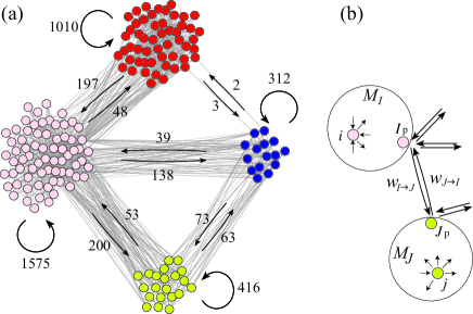
Most directed networks in the real world are more structured than those captured by the MA. A ubiquitous global structure of networks is modular structure. Modular networks consist of several densely connected subgraphs called modules (also called communities), and modules are connected to each other by relatively few links. As an example, a subnetwork of the C. elegans neural network [43, 44] containing 4 modules is shown in Fig. 1(a). Modular structure is common in both undirected [21, 22, 23, 24] and directed [24, 25, 26, 27] networks.
Modular structure of directed networks often leads to hierarchical structure. By hierarchy, we refer to the situation in which modules are located at different levels in terms of the value of the ranking-type centrality. It is relatively easy to traverse from a node in an upper level to one in a lower level along directed links, but not vice versa. The hierarchical structure leads to the deviation of from the value obtained from the MA.
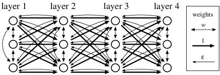
As an example, consider the directed -partite network shown in Fig. 2. Layer () contains nodes, where is divided by . The nodes in the same layer are connected bidirectionally with weight . Each node in layer () sends directed links to all nodes in layer with weight unity, and each node in layer () sends directed links to all the nodes in layer with weight . The following results do not change if two adjacent layers are connected via just an asymmetrically weighted bridge, as shown in Fig. 1(b). Because of the symmetry, all nodes in layer have the same influence . From Eq. (1), we obtain
| (8) |
When , a node in a layer with small is more influential than a node in layer with large . The MA yields
| (9) |
The actual decreases exponentially throughout the hierarchy, whereas does not. We observe a similar discrepancy in the case of the PageRank.
We develop an improved approximation for the influence in modular networks by combining the MA and the correction factor obtained from the global modular structure of networks. Consider a network of modules (). For mathematical tractability, we assume that each module communicates with the other modules via a single portal node , as illustrated in Fig. 1(b); the network shown in Fig. 1(b) is an approximation of that shown in Fig. 1(a). We denote the weight of the link by ().
We obtain in this modular network by enumerating spanning trees rooted at node . Denote such a spanning tree by . The intersection of and is a spanning tree restricted to and rooted at node . This restricted spanning tree reaches all nodes in . enters () via a directed path from node to node . This path is provided by a spanning tree in the network of modules, where each module is represented by a single node. The other nodes in are spanned by the intersection of and , which forms a spanning tree restricted to and rooted at node . Therefore, is a concatenation of (i) an intramodular spanning tree in and rooted at node , (ii) intramodular spanning trees in and rooted at node (), and (iii) a spanning tree in the network of modules rooted at node . Let ( for local) denote the number of spanning trees in with an arbitrary root, and ( for global) denote the number of spanning trees in a network of modules with an arbitrary root. Then, the number of spanning trees in rooted at node is equal to
| (10) |
where is the influence of node within and is the influence of in the network of modules. The first, second, and third factors in Eq. (10) corresponds to the numbers of spanning trees of types (i), (ii), and (iii), respectively. Therefore, we obtain
| (11) |
For nodes , Eq. (11) yields ; the relative influence of nodes in the same module is equal to their relative influence within the module. For nodes in different modules, i.e., node in module and node in module (), Eq. (11) leads to
| (12) |
If each module is homogeneous, we approximate , and obtain ; the global structure of the network laid out by links across modules determines the influence of each node. If each module is heterogeneous in degree, we use the MA, i.e., and . By assuming that () is a typical node in (), we set and . Then, Eq. (12) is transformed into
| (13) |
Therefore, we define an approximation scheme, called the MA-Mod, for node in module as
| (14) |
Equation (14) can be used for general modular networks in which different modules can be connected by more than one links.
Two crucial assumptions underlie Eq. (14). Firstly, a module is assumed to be an uncorrelated and possibly heterogeneous random network so that the MA is effective within the module. Note that the degree of nodes can be heterogeneously distributed. Secondly, most links are assumed to be intramodular so that the local MA is simply given by .
4 Application to Real Data
We examine the effectiveness of the MA-Mod scheme using three datasets from different fields.
4.1 Neural network
In the network of nematode C. elegans, a pair of neurons may be connected by chemical synapses, which are directed links, or gap junctions, which are undirected links. We calculate the influence of neurons on the basis of a connectivity dataset [43, 44]. The link weight is assumed to be the sum of the number of chemical synapses from neuron to neuron and that of the gap junctions between neuron and neuron . The following results are qualitatively the same if we ignore the gap junction or the link weight (see Appendix C for the results). The largest strongly connected component, which we simply call the neural network, contains nodes and links.
It is difficult to determine whether the influence or the PageRank is more appropriate from current biological evidence. If postsynaptic neurons linearly integrate different synaptic inputs, the influence may be an appropriate measure. In contrast, postsynaptic neurons may effectively select one synaptic input by a nonlinear mechanism. If each input is selected with the same probability in a long run and the activity level does not differ much across neurons, the PageRank may be appropriate. We examine both scenarios using power iteration (see Appendix D for the methodology).
Among 274 neurons, 54, 79, and 87 neurons are classified as sensory neurons, interneurons, and motor neurons, respectively [44]. By definition, sensory neurons directly receive external input such as touch and chemical substances, motor neurons send direct commands to move the body, and interneurons mediate information processing in various ways. The other neurons are polymodal neurons or neurons whose functions are unknown. Neurons with a large are mostly sensory neurons. For example, among the 10 neurons with the largest , 8 are sensory neurons (ALMR, ASJL, ASJR, AVM, IL2VL, PHAL, PHAR, PVM) and 2 are interneurons (AIML, AIMR). Generally speaking, these neurons have a large not simply because their is large. The average of over the 10 neurons is equal to 3.456 (see Tab. A2 in Appendix C for the values for individual neurons). These neurons are located at upper levels of the neural network in the global sense. The conclusion remains qualitatively the same if we use . Recall that the PageRank is calculated for because the meaning of the direction of the link in the influence is opposite to that in the PageRank.
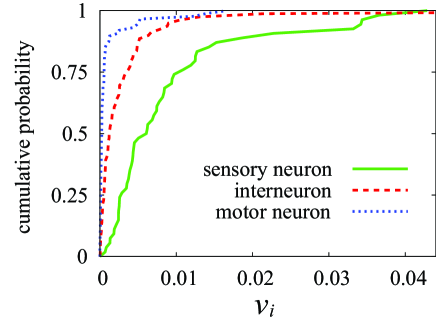
The average values of () for sensory neurons, interneurons, and motor neurons are equal to 0.009235 (0.006621), 0.003614 (0.005415), and 0.001032 (0.001323), respectively. The cumulative distributions of for different classes of neurons are shown in Fig. 3. Even though many synapses from motor neurons to interneurons and sensory neurons, and synapses from interneurons to sensory neurons exist, these numerical results indicate that the neural network is principally hierarchical. Generally speaking, sensory neurons, which directly receive external stimuli, are located at upper levels of the hierarchy, motor neurons are located at lower levels, and interneurons are located in between. Sensory neurons serve as a source of signals flowing to interneurons and motor neurons down the hierarchy.
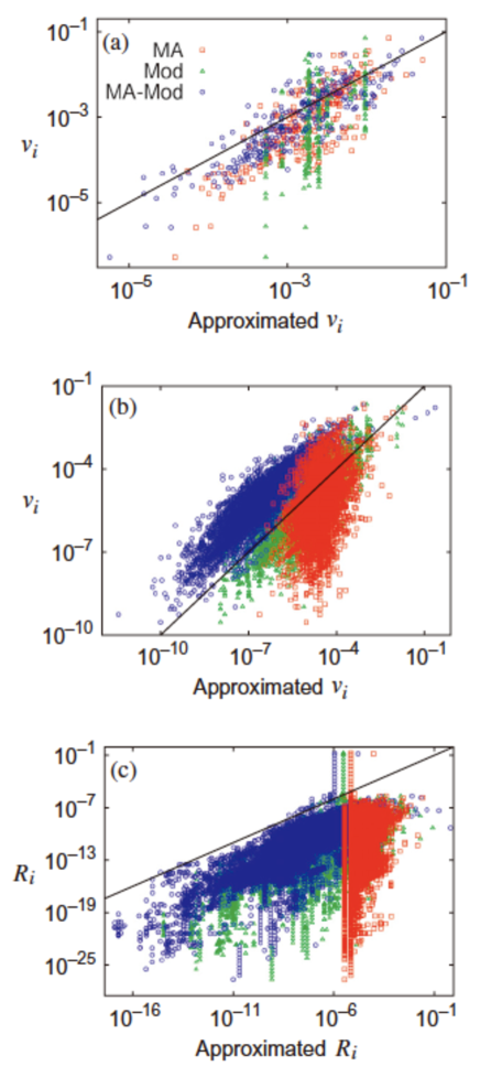
The relation between and the MA is shown in Fig. 4(a) by the squares. They appear strongly correlated. However, the Pearson correlation coefficient (PCC; see Appendix E for definition) between and the MA is not large (), as shown in Tab. 1, because tends to be larger than the MA for nodes with a large . Note that the data are plotted in the log-log scale in Fig. 4.
The neural network has modular structure [45]. To use the MA-Mod scheme (Eq. (14)), we apply a community detection algorithm [27] to the neural network. We have selected this algorithm [27] because a directed link in the present context indicates the flow rather than the connectedness on which a recent algorithm [26] is based. As a result, we obtain modules, calculate , , from the network of the modules, and use Eq. (14). is plotted against the MA-Mod in Fig. 4(a), indicated by circles. The data fitting has improved compared to the case of the MA, in particular for small values of . The PCC between and the MA-Mod is larger than that between and the MA (Tab. 1). In this example, this holds true for the raw data and the logarithmic values of the raw data. As a benchmark, we assess the performance of the global estimator (node ), which we call the Mod. The Mod ignores the variability of within the module and is exact for networks with completely homogeneous modules, such as the network shown in Fig. 2. The performance of the Mod is poor in the neural network, as indicated by the triangles in Fig. 4(a) and the PCC listed in Tab. 1.
The values of the PCC between the actual and approximated are also listed in Tab. 1. The results for the PageRank are qualitatively the same as those for the influence. With both measures, the module membership is a crucial determinant of centralities of individual nodes. Note that, on the basis of the Mod for the influence given by
| (19) |
the Mod for the PageRank is given by
| (20) |
i.e.,
| (21) |
We approximate by because the information about local degree is unavailable for the Mod.
| network | C. elegans | WWW | |||||
| 274 | 9079 | 53968 | |||||
| 13 | 637 | 2977 | |||||
| centrality | |||||||
| N/A | 0 | N/A | 0 | N/A | 0 | 0.15 | |
| MA | 0.5389 | 0.3593 | 0.5066 | 0.3997 | 0.0073 | 0.0007 | 0.2162 |
| Mod | 0.2927 | 0.4346 | 0.5010 | 0.2452 | 0.0003 | -0.0003 | 0.4104 |
| MA-Mod | 0.7295 | 0.5005 | 0.5066 | 0.2671 | 0.0000 | 0.0000 | 0.3166 |
| MA (log) | 0.8024 | 0.7073 | 0.3636 | 0.5353 | 0.3109 | 0.1289 | 0.4627 |
| Mod (log) | 0.5195 | 0.5503 | 0.8075 | 0.7147 | 0.7800 | 0.7147 | 0.4098 |
| MA-Mod (log) | 0.8736 | 0.8252 | 0.8798 | 0.9022 | 0.7964 | 0.7812 | 0.6256 |
4.2 Email social network
Our second example is the largest strongly connected component of an email social network [46]. A directed link exists between a sender and a recipient of an email. The network has modular structure [25]. In the weighted network that we consider here, the link weight is defined by the number of emails. The following results do not qualitatively change even if we neglect the link weight (see Appendix F). The largest strongly connected component has 9079 nodes and 23808 links and is partitioned into 637 modules.
Whether the influence or the PageRank is appropriate for ranking nodes depends on the assumption about human behavior. If recipients spend the same amount of time on each incoming email (i.e., the link of weight unity), is relevant. In contrast, recipients may have a fixed amount of time for dealing with all incoming emails. Then, a recipient may equally distribute the total time available to each email depending on the number of incoming emails. Under this assumption, the PageRank is relevant. We analyze both and .
In Fig. 4(b), the values of are plotted against those obtained by different estimators. On the log-log scale, the MA-Mod performs considerably better than the MA. Remarkably, even the Mod, in which nodes in the same module share an estimated centrality value, performs better than the MA. This is a strong indication that the structure of the coarse-grained network of modules is a more important determinant of than the local structure (i.e., degree) in this example. The values of the PCC summarized in Tab. 1 support our claim. The PCC for the MA-Mod and the Mod is considerably larger than that for the MA on the logarithmic scale, which implies that the MA-Mod is especially effective for nodes with small . The values of the PCC between and the different estimators are listed in Tab. 1. These results are qualitatively the same as those for .
4.3 WWW
Our last example is the largest strongly connected components of a WWW dataset [47]. The original network contains 325729 nodes and 1469680 links, and the largest strongly connected component contains 53968 nodes and 296229 links. The MA fits the PageRank (with ) of some WWW data when nodes of the same degree are grouped together [17] but not other data [18]. Because of the modular structure of the WWW [25], the MA-Mod is expected to perform better than the MA.
In Fig. 4(c), for is plotted against the MA, Mod, and MA-Mod. For nodes with small PageRanks, the MA-Mod, and even the Mod, are considerably better correlaed with than the MA is (note the use of the log-log scale in Fig. 4(c); also see Tab. 1). These nodes are located at lower levels of hierarchy. The results are qualitatively the same if we use the influence (Tab. 1). Note that we reverse the links and calculate because a directed link in the WWW indicates an impact of the target node on the source node.
The MA-Mod for the PageRank can be extended to the case . From Eq. (2), the MA for the PageRank is given by
| (22) |
which implies that in the MA for is replaced by for general . We define the MA-Mod for by
| (23) |
Note that this ansatz is heuristic, whereas Eq. (17) used for has an analytical basis. The PCCs between the PageRank with and the three estimates are listed in Tab. 1. The MA-Mod performs better than the MA. The advantage of the MA-Mod over the MA is smaller for than for because a larger implies a heavier neglect of the network structure.
The definition of the PageRank given by Eq. (2) is not continuous with respect to the outdegree; the term is present for (i.e., dangling node) and absent for . Therefore, dangling nodes can have large PageRanks. To improve the MA-Mod for , we should separately treat dangling nodes and other nodes in the same module. We do not explore this point because this situation seems to be specific to the working definition of the PageRank.
In practice, nodes with a small could be irrelevant to the performance of a search engine, which outputs a list of websites with the largest PageRanks. However, nodes with small PageRanks constitute the majority of a network when the PageRank follows a power-law distribution. This is the case for the real WWW data, which are scale-free networks [17, 18]. Our method is considerably better than the MA especially for nodes with small PageRanks.
In general, the WWW is nested, with each level defined by webpages, directories, hosts, and domains. At the host level, for example, most links are directed toward nodes within the same host [48]. Therefore, a host can be regarded as a module in the network. By calculating the importance of the host, called the BlockRank, the PageRank can be efficiently computed [48]. In spirit, our is similar to the BlockRank, although our is used for identifying the hierarchical levels of networks and systematically approximating .
It should be noted that, in general, our approximation scheme runs much faster than the direct calculation of or for large networks. This is because the community detection algorithm [27] is fast and the power iteration used for calculating and converges faster for a smaller network in most (but not all) cases. In the WWW, which is a large network, our approximation scheme for the PageRank with ran more than 100 times faster than the direct calculation on our computer.
5 Discussion and Conclusions
We have shown that the hierarchical structure of directed modular networks considerably affects ranking-type centrality measures of individual nodes. Using the information about connectivity among modules, we have significantly improved the estimation of centrality values. Our theoretical development is based on the measure that we have proposed (i.e., influence), but the conclusions hold true for both the influence and the PageRank. Our method can be implemented for variants of the PageRank including the eigenfactor [14, 15] and the so-called invariant method [11, 13] used for ranking academic journals.
The hierarchy discussed in this study is different from the nestedness of networks. Many networks are hierarchical in the sense that they are nested and have multiple scales [30, 31, 32, 33]. A modular network is hierarchical in this sense, at least to a limited extent; two hierarchical levels are defined by the scale of the entire network and that of a single module. In contrast, we are concerned with hierarchical relationships among modules defined by the directionality of networks. This concept of hierarchy has been studied for, for example, food webs [4], transcription networks [5], and social dynamics [6], but its understanding based on networks is relatively poor in spite of its intuitive appeal. The influence and the PageRank quantify the hierarchical position of individual nodes and of modules.
In real networks, nodes and links are subjected to changes. Such changes affect nodes near the perturbed nodes, but may not significantly affect modules. In social networks, large groups change slowly over time as compared to small groups [23]. In addition, in the absence of complete knowledge of networks, modest understanding of networks at the level of the modular structure may be adequate. Nodes in a module may also have a common function. These are main reasons behind investigating the modular structure of networks. We have shown that the modular structure is also important in the context of directed networks, hierarchy, and ranking. The definition of module is complex in the case of directed networks as compared to undirected networks, and module detection in directed networks is currently under investigations (see [24] for a review). We hope that our results aid the development of the concept of modules and related algorithms in directed networks.
Acknowledgments
We thank Jesper Jansson and Kei Yura for their valuable discussions. N.M. acknowledges the support through the Grants-in-Aid for Scientific Research (Nos. 20760258 and 20540382) from MEXT, Japan.
Appendix A: Influence is obtained from various dynamical models on networks
Fixation probability of evolutionary dynamics
represents the probability that an ‘opinion’ introduced at node spreads to the entire network. We consider stochastic competitive dynamics between two equally strong types of opinions and ; each node takes either or at a given time. In the so-called link dynamics (LD) [39, 40], which is a network version of the standard voter model, one link is selected for reproduction with an equal probability in each time step. Then, the type at node replaces that at node . This process is repeated until or takes over the entire network.
coincides with the fixation probability denoted by , which is the probability that a new type introduced at node in the network of the resident type nodes takes over the entire network [20]. To calculate , fix a network and consider the initial configuration in which is located at node and is located at the other nodes. In the first time step, one of the following events occurs. With the probability , the link is selected for reproduction. Then, type is located at nodes and . Let denote the fixation probability of type for this new configuration. With the probability , the link is selected, type becomes extinct, and the dynamics terminates. With the remaining probability , the configuration of types and on the network does not change. Therefore, we obtain
| (24) |
Continuous-time simple random walk
Consider a simple random walk on the network in continuous time. In a small time interval , a walker at node is attracted to its neighbor , where , with the probability . Note that the direction of the link is opposite to the convention because the directed link in the present study indicates the influence of the source node of the link on the target node of the link. The master equation for the density of the random walker at node , denoted by (), is represented by
| (25) |
Because the network is strongly connected, converges to the unique stationary density. By setting the LHS of Eq. (25) to 0, we obtain .
The simple random walk is closely associated with the fixation problem. The so-called dual process of the LD is the coalescing random walk. In the coalescing random walk, each of the walkers basically performs the continuous-time simple random walk on the network with the direction of all links reversed. Therefore, the random walker can traverse from node to node when . If two random walkers meet on a node, they coalesce into one walker. There is only one walker after sufficiently long time, and the duality between the two stochastic processes guarantees [20].
Reproductive value
DeGroot model in social dynamics
The DeGroot model [35, 36, 37] is a discrete-time model that represents the propagation of information or opinions in social systems. The state of the individual at node is represented by a real value ; parameterizes the information that the individual at node has at time . The weight is the probability that the individual at node copies the opinion at node in the next time step. The normalization is given by . The states of the nodes evolve according to
| (26) |
If the network is strongly connected and aperiodic, a consensus is reached asymptotically, i.e., [36, 37].
The extent to which the initial information at node influences the limiting common information in the continuous-time version of the DeGroot model is equal to . To show this, we start with the discrete-time dynamics given by Eq. (26). Suppose that () satisfies for arbitrary . Because the configuration and the configuration starting with end up with the identical , we obtain
| (27) |
Since are arbitrary, we obtain
| (28) |
Equation (28) is of the same form as Eq. (1). However, the condition is imposed in Eq. (28) because the dynamics are defined in the discrete time. The continuous-time counterpart of the DeGroot model is defined in [37] as follows:
| (29) |
If , we obtain , which leads to
| (30) |
for arbitrary . Therefore, .
Collective responses in coupled oscillator dynamics
According to [38], consider coupled phase oscillators obeying
| (31) |
where is the phase of the oscillator , is the intrinsic frequency of the oscillator , is the effect of node on node , and is the input at time applied to node . We assume that (i) in the absence of the input (i.e., ), the system is fully phase-locked, i.e., for all with some constants and and that (ii) the input is small, i.e., , so that the system is always close to the phase-locked state. Using the synchronization condition, i.e., (), which is implied by assumption (i), we linearize Eq. (31) as
| (32) |
where is a small perturbation in the phase, and is the Jacobian matrix given by . Note that the effective weight of the link from node to node is given by . Because assumption (i) implies the stability of the phase-locked state, the real parts of all the eigenvalues of are negative, except a zero eigenvalue. We define the collective phase by . Combination of (), which is derived from Eq. (1), and Eq. (32) yields
| (33) |
Assumption (ii) implies that . Therefore, Eq. (33) describes the dynamical behavior of each oscillator and that of the entire network. The response of the collective behavior to the input applied to node is weighted by .
Appendix B: Relationship between the influence and the PageRank
To determine the relationship between the influence and the PageRank, we rewrite Eq. (2) as
| (34) |
From the original network , define a complete and asymmetrically weighted network using the matrix of link weights . Because (), in is equal to in , which we denote by for clarity. Because self loops do not affect the calculation of the influence, we can replace by .
In particular, for is equal to , where is defined by . In this case, the PageRank and the influence are connected by the simple relationship given by Eq. (3).
Appendix C: Detailed analysis of the C. elegans neural network
The relative contribution of a chemical synapse and that of a gap junction to signal transduction in the C. elegans neural circuitry are unknown. In the main text, we have assumed that the neural network is a weighted network in which a chemical synapse has the same link weight as a gap junction. Here we examine three other variants of C. elegans neural networks. In these three neural networks, we neglect the link weight and/or gap junctions. The omission of the link weight reflects the possibility that the intensity of the communication between two neurons may saturate as the number of synapses increases. The omission of gap junctions reflects the possibility that gap junctions may not contribute to signal processing as significantly as chemical synapses. Note that the largest strongly connected component shrinks to a network of 237 nodes with 1936 synapses by the omission of gap junctions.
For the three neural networks, the values of the PCC between the centralities of the nodes and the three approximators are listed in Tab. A1. We have examined both and with . In general, the MA-Mod predicts and better than the MA in the three networks. The results listed in Tab. A1 are consistent with those presented in the main text.
For the four neural networks, including the one in the main text, the 10 most influential neurons are listed in Tab. A2. This list of 10 neurons is largely consistent across different definitions of neural network. For the majority of these neurons, is larger than the value predicted from the MA.
Appendix D: Power iteration
If we use a standard numerical method such as the Gaussian elimination, the computation time required for calculating and from Eqs. (1) and (2), respectively, is . For sparse networks, carrying out power iteration (also called Jacobi iteration) may be much faster. The convergence of this iteration is guaranteed, as explained below for the influence. The proof for the PageRank is almost the same.
We rewrite Eq. (1) as
| (35) |
Equation (35) indicates that is the -th element of the right eigenvector of the matrix for the eigenvalue equal to unity. Multiplying by the diagonal matrix on the right and its inverse on the left does not alter the spectrum of . This operation yields a new matrix whose () element is given by . The spectral radius of the new matrix is at most unity because its maximum row sum matrix norm [49, p.295] is equal to unity. Consequently, the spectral radius of is equal to unity.
Consider the power iteration scheme in which the -th estimate of () is given by the RHS of Eq. (35) in which the -th estimate of () is substituted. If the network is strongly connected and aperiodic, the nonnegative matrix is primitive, i.e., the eigenvalue of the largest modulus, which is equal to unity in the present case, is unique [49, p.516]. Then, the convergence of power iteration to the correct is guaranteed [49, p.523]. The Perron-Frobenius theorem [49] guarantees that the Perron vector is uniquely determined and that (). The power iteration converges quickly if the modulus of the second eigenvalue of is considerably smaller than that of the largest eigenvalue, i.e., unity.
Appendix E: PCC
The PCC between and an estimator , such as MA, Mod, and MA-Mod, is defined by
| (36) |
Note that .
Appendix F: Results for unweighted email social network
The values of the PCC between the two centrality measures and different estimators for the unweighted email social network are listed in Tab. A3. The results are qualitatively the same as those for the weighted network shown in the main text.
| gap junction | yes | no | no | |||
|---|---|---|---|---|---|---|
| link | unweighted | weighted | unweighted | |||
| 274 | 237 | 237 | ||||
| 7 | 20 | 15 | ||||
| centrality | ||||||
| MA | 0.7420 | 0.6331 | 0.2145 | 0.0875 | 0.5153 | 0.4240 |
| Mod | 0.3727 | 0.2542 | 0.1577 | 0.1741 | 0.1583 | 0.2224 |
| MA-Mod | 0.8235 | 0.7401 | 0.3328 | 0.1189 | 0.4949 | 0.4659 |
| MA (log) | 0.8478 | 0.7942 | 0.6899 | 0.6152 | 0.7976 | 0.7726 |
| Mod (log) | 0.5190 | 0.1937 | 0.7018 | 0.7338 | 0.6743 | 0.6519 |
| MA-Mod (log) | 0.8995 | 0.8752 | 0.8475 | 0.8137 | 0.8785 | 0.8586 |
| with gap junction | with gap junction | no gap junction | no gap junction | ||||||||
|---|---|---|---|---|---|---|---|---|---|---|---|
| weighted | unweighted | weighted | unweighted | ||||||||
| neuron | neuron | neuron | neuron | ||||||||
| AIMR | 0.08876 | 4.160 | PHAL | 0.04279 | 3.226 | AIMR | 0.06841 | 3.924 | VC04 | 0.05899 | 4.594 |
| ASJL | 0.04287 | 3.588 | PHAR | 0.04117 | 3.449 | ASJL | 0.04835 | 3.467 | VC05 | 0.04439 | 3.841 |
| ALMR | 0.03657 | 3.296 | AIMR | 0.04062 | 2.356 | ALMR | 0.03965 | 2.843 | AIMR | 0.03718 | 2.227 |
| PHAR | 0.03435 | 7.740 | ASIL | 0.02748 | 2.072 | VC04 | 0.03334 | 2.988 | AIML | 0.02722 | 1.325 |
| PHAL | 0.03419 | 6.259 | ASIR | 0.02695 | 2.540 | PVM | 0.03246 | 2.116 | AWAL | 0.02715 | 1.510 |
| ASJR | 0.03319 | 4.094 | AIML | 0.02152 | 1.432 | AVM | 0.02847 | 1.047 | AVG | 0.02426 | 2.951 |
| IL2VL | 0.02647 | 0.456 | IL2VL | 0.02061 | 0.706 | AIML | 0.02304 | 2.447 | AVM | 0.01715 | 1.028 |
| AVM | 0.02273 | 1.816 | ALMR | 0.01982 | 2.135 | AVG | 0.02257 | 8.826 | ASKR | 0.01701 | 3.975 |
| AIML | 0.02133 | 2.231 | VC05 | 0.01719 | 2.160 | ASJR | 0.02217 | 2.649 | ALMR | 0.01692 | 1.647 |
| PVM | 0.01860 | 1.816 | VC04 | 0.01505 | 2.838 | ADLL | 0.01777 | 0.593 | IL2VL | 0.01546 | 0.669 |
| 9079 | ||
|---|---|---|
| 599 | ||
| centrality | ||
| N/A | 0 | |
| MA | 0.6628 | 0.5536 |
| Mod | 0.6537 | 0.3290 |
| MA-Mod | 0.6692 | 0.4774 |
| MA (log) | 0.2552 | 0.4203 |
| Mod (log) | 0.8719 | 0.7754 |
| MA-Mod (log) | 0.8898 | 0.9042 |
References
- [1] Wasserman S and Faust K 1994 Social Network Analysis (New York: Cambridge University Press)
- [2] Newman M. E. J. 2003 SIAM Rev. 45 167
- [3] Boccaletti S, Latora V, Moreno Y, Chavez M and Hwang D-U 2006 Phys. Rep. 424 175
- [4] Garlaschelli D, Caldarelli G and Pietronero L 2003 Nature 423 165
- [5] Lagomarsino M C, Jona P, Bassetti B and Isambert H 2007 Proc. Natl. Acad. Sci. USA 104 5516
- [6] Castellano C, Fortunato S and Loreto V 2009 Rev. Mod. Phys. 81 591
- [7] Brin S and Page L 1998 Proc. 7th Int. World Wide Web Conf. (Brisbane, Australia, 14–18 April) 107–117.
- [8] Berkhin P 2005 Internet Math. 2 73
- [9] Kleinberg J M 1999 J. ACM 46 604
- [10] Kleinberg J and Lawrence S 2001 Science 294 1849
- [11] Palacios-Huerta I and Volij O 2004 Econometrica 72 963
- [12] Chen P, Xie H, Maslov S and Redner S 2007 J. Informetrics 1 8
- [13] Pinski G and Narin F 1976 Info. Proc. Man. 12 297
- [14] Davis P M 2008 J. Amer. Soc. Info. Sci. Tech. 59 2186
- [15] Fersht A 2009 Proc. Natl. Acad. Sci. USA 106 6883
- [16] Park J and Newman M E J 2005 J. Stat. Mech. P10014
- [17] Fortunato S, Flammini A, Menczer F and Vespignani A 2006 Proc. Natl. Acad. Sci. USA 103 12684
- [18] Donato D, Laura L, Leonardi S and Millozzi S 2004 Eur. Phys. J. B 38 239
- [19] Restrepo J G, Ott E and Hunt B R 2006 Phys. Rev. Lett. 97 094102
- [20] Masuda N and Ohtsuki H 2009 New. J. Phys. 11 033012
- [21] Newman M E J 2004 Eur. Phys. J. B 38 321
- [22] Palla G, Derényi I, Farkas I and Vicsek T 2005 Nature 435, 814
- [23] Palla G, Barabási L-A and Vicsek T 2007 Nature 446 664
- [24] Fortunato S 2009 Phys. Rep. in press. arXiv:0906.0612v1
- [25] Palla G, Farkas I J, Pollner P, Derényi I and Vicsek T 2007 New J Phys 9 186
- [26] Leicht E A and Newman M E J 2008 Phys. Rev. Lett. 100 118703
- [27] Rosvall M and Bergstrom C T 2008 Proc. Natl. Acad. Sci. USA 105 1118
- [28] Everett M G and Borgatti S P 1999 J. Math. Sociol. 23 181
- [29] Taylor P D 1990 Amer. Natur. 135 95
- [30] Ravasz E, Somera A L, Mongru D A, Oltvai Z N and Barabási A-L 2002 Science 297 1551
- [31] Guimerà R and Amaral L A N 2005 Nature 433 895
- [32] Sales-Pardo M, Guimerà R, Moreira A A and Amaral L A N 2007 Proc. Natl. Acad. Sci. USA 104 15224
- [33] Clauset A, Moore C, Newman M E J 2008 Nature 453 98
- [34] Taylor P D 1996 J. Math. Biol. 34 654
- [35] DeGroot M H 1974 J. Am. Stat. Asso. 69 118
- [36] Jackson M O 2008 Social and Economic Networks (Princeton: Princeton University Press)
- [37] Olfati-Saber R, Fax J A and Murray R M 2007 Proc. IEEE 95 215
- [38] Kori H, Kawamura Y, Nakao H, Arai K and Kuramoto Y 2009 Phys. Rev. E 80 036207
- [39] Antal T, Redner S and Sood V 2006 Phys. Rev. Lett. 96 188104
- [40] Sood V, Antal T and Redner S 2008 Phys. Rev. E 77 041121
- [41] Biggs N 1997 Bull. L. Math. Soc. 29 641
- [42] Agaev R P and Chebotarev P Y 2000 Autom. Rem. Cont. 61 1424
- [43] Chen B L, Hall D H and Chklovskii D B 2006 Proc. Natl. Acad. Sci. USA 103 4723
- [44] http://www.wormatlas.org
- [45] Müller-Linow M, Hilgetag C C and Hütt M-T 2008 PLoS Comput. Biol. 4 e1000190
- [46] Ebel H, Mielsch L-I and Bornholdt S 2002 Phys. Rev. E 66 035103(R)
- [47] Albert R, Jeong H and Barabási A-L 1999 Nature 401 130
- [48] Kamvar S D, Haveliwala T H, Manning C D and Golub G H 2003 In: Proc 12th Int World Wide Web Conf, May 2003.
- [49] Horn R A and Johnson C R 1985 Matrix Analysis (Cambridge: Cambridge University Press).