Thermal Equilibrium of Hagedorn and Radiation Regimes in String Gas Cosmology

Abstract

In this paper, we investigate thermal equilibrium in string gas cosmology which is dominated by closed string. We consider two interesting regimes, Hagedorn and radiation regimes. We find that for short strings in small radius of Hagedorn regime very large amount of energy requested to have thermal equilibrium but for long strings in such system a few energy is sufficient to have thermal equilibrium. On the other hand in the large radius of Hagedorn regime, which pressure is not negligible, we obtain a relation between the energy and pressure in terms of cosmic time which is satisfied by thermal equilibrium. Then we discuss about radiation regime and find that in all cases there is thermal equilibrium.

Keywords: String Gas Cosmology; Dilaton - Gravity; Closed String; Thermodynamics.

1 Introduction

String gas cosmology [1] is one of the best model of the early universe, which is called Brandenberger - Vafa (BV) scenario. This model claimed that the early universe was small and compact and surrounded by hot and high dense string gas. Because of vanishing winding modes of strings, (A closed string can wrap around the extra dimension, such a state is called a winding mode and is appropriate with inverse of extra dimension, ie. $\omega\sim 1/R$), three dimensions of space become large ($\omega\rightarrow 0\Rightarrow R\rightarrow\infty$). For more studying one may see several papers [2-13]. One of the important problem in this model is consideration of thermal equilibrium in the early universe. In that case the early time cosmic evolution in string gas cosmology considered by means of open strings attached to $D$-branes [14]. In that paper, statistical properties of open strings in $D$-brane background reviewed and string fields determined by using dilaton - gravity equations in the Hagedorn regime. Authors in Ref. [14] concluded that initial conditions can be fine tuned to have thermal equilibrium in the beginning, but, in a short time, string gas falls out of thermal equilibrium. Through the similar method of Ref. [14] dominated by closed strings, we study thermal equilibrium in string gas cosmology. In this way we perform different calculation with the Ref. [15] about the interaction rate.
In the Ref. [16] some aspects of string gas cosmology at finite temperature described for two cases, (I) Hagedorn regime in a very small homogeneous and isotropic universe, (II) a radiation regime with two independent scale factors corresponding to large and small dimensions. In the radiation regime the lightest Kaluza - Klein and winding mode contributions considered. It is known that in both Hagedorn and radiation regimes some matters have manifestly $T$-duality invariant. Importance of the radiation regime explained well in the Ref. [16], therefore we are interest to consider this regime to study of thermal equilibrium in the early universe.
As we told, Open strings and Hagedorn regime in string gas cosmology studied [14]. Here, we follow same way and consider thermodynamics of string gas in the early universe which is dominated by the closed strings. We study thermal equilibrium condition for the early time of the universe in Hagedorn and radiation regime. We take equations of motion from Ref. [16] and solve them in the way of Ref. [14] and explain requirements of thermal equilibrium.
This paper organized as the following. In the section 2 we review thermodynamics of closed strings and write the relevant entropy for the small and large radius. Then in the section 3 we consider dilaton - gravity in the Hagedorn regime with a single scale factor, and study thermal equilibrium by calculating Hubble parameter and the interaction rate. In the section 4 we repeat analysis of the section 3 in the almost-radiation regime and with two scale factors. Finally in the section 5 we give conclusion and discussion of the thermal equilibrium in the early universe.

2 The closed string entropy

In this section we review the calculation of the closed strings entropy in dilaton - gravity background. We assume that all of directions are small and compact, which represented by a flat $T^{9}$ torus. Also we would like to consider our system at temperature close to the Hagedorn temperature and in low - energy limit. Therefore there are $D=9$ compact coordinates which are represented by $x_{i}$ with $i=1,2...9$. The space - time metric and dilaton field may be written as the following,

$$ds^{2} = -dt^{2}+R_{i}^{2}dx^{2},$$

$$R_{i} = e^{\lambda_{i}(t)},$$

$$\phi = \phi(t),$$ (1)

where $R_{i}$ $(i=1,2...,9)$ denote the scale-factor of the torus and are equal to the corresponding radii for the world - volume. So, one can define the volume of the space by $V=(R_{i})^{D}$. Because of the string T-duality ($R\rightarrow 1/R$ symmetry ) we can take all dimensions to be larger than string scale, ie. $R_{i}\geq 1$, moreover we set $\alpha^{\prime}=1$ for convenient. By consideration of the closed string model we want to study the early time cosmic evolution in string gas cosmology. In the microcanonical ensemble there is a critical temperature which is called the Hagedorn temperature [17], where the partition function of a free string gas diverges. Therefore in this regime the usual thermodynamical equivalence between the canonical and microcanonical ensembles can break down and more fundamental ensemble must be used. We use different methods from Ref. [16] to obtain the entropy. By using density of single string state [18] we will obtain thermodynamics of the closed strings. The closed string energy $\varepsilon$ corresponds to the length of random walk and the number of them grow with factor $\exp(\beta_{h}\varepsilon)$, where $\beta_{h}$ is inverse of the Hagedorn temperature. Also there is a volume factor of random walk $V_{walk}=W$. In addition there is a factor $V$ to transformation of zero state and a factor $1/\varepsilon$ because of periodic nature of the closed strings. In order to specify the single string density of states we must account all of above factors which yield to the following expression,

$$\omega(\varepsilon)\sim\frac{V\exp(\beta_{h}\varepsilon)}{\varepsilon W}.$$ (2)

By using the T-duality in string theory, the small and compact space has dual picture as non-compact space, hence we consider two following cases:
(i) $R_{i}\ll\sqrt{\varepsilon}$, it is small radius regime and all of directions are effectively compact which is called space-filling. In this case one can find $\omega(\varepsilon)=\frac{\exp(\beta_{h}\varepsilon)}{\varepsilon}$.
(ii) $R_{i}\gg\sqrt{\varepsilon}$, it is large radius regime and all of directions are effectively non-compact which is called well-contained. In this case one can find, $\omega(\varepsilon)={V\exp(\beta_{h}\varepsilon)}{\varepsilon^{D^{\prime}}}$, where $D^{\prime}=-\frac{D+1}{2}$. In the small radius regime, where $\varepsilon\gg 1$, the value of energy is sufficient to excite winding modes of closed string, but in the large radius regime, where $\varepsilon\ll 1$, the value of energy is lower than excitation of winding modes. Then the total density of states, $\Omega(E)$, is given by [14],

$$\Omega(E)=\Sigma_{k}\frac{1}{k!}\prod_{i=1}^{k}\int_{0}^{E}\Omega(\varepsilon_{i})d\varepsilon_{i}\delta(\Sigma{\varepsilon_{i}}-E),$$ (3)

where $k$ is the number of strings. The equation (3) can be rewritten in the form of the following expression,

$$\Omega(E)=\frac{1}{2\pi E}\int_{-\infty}^{\infty}d\alpha e^{-i\alpha}e^{F(\alpha)},$$ (4)

where $F(\alpha)$ is defined as,

$$F(\alpha)=\int_{0}^{E}d\varepsilon\omega(\varepsilon)e^{\frac{i\alpha\varepsilon}{E}}.$$ (5)

We must note that $F(\alpha)$ is a regular function which vanishes at $\alpha\rightarrow\pm\infty$ limit, and therefore the integral (4) is not divergent. In order to obtain entropy we calculate the integral (4) in both small and large radius. In the first case, small radius, one can obtain $F(\alpha)=\ln E+\gamma E$, where $\gamma=\frac{\beta_{h}E+i\alpha}{E}$. Therefore entropy is is given by $S=ln\Omega(E)\simeq\beta_{h}E$. Similarly in the second case for large radius, one can obtain,

$$S=\beta_{h}E+\ln\frac{z^{n}}{n!(n+D^{\prime})!}$$ (6)

where, $z=-(-1)^{D^{\prime}}D^{\prime}!VE^{D^{\prime}}$, and for $D=9$ it reduces to $z=-120VE^{-5}$. In the next sections we use above information to study the thermal equilibrium of a given system.

3 Dilaton gravity and Hagedorn regime

In this section we shall study the dilaton - gravity equations of motion with a massless dilaton field $\Phi$ corresponding to the low-energy effective action of string theory in $D+1$ space-time dimension [14,19] at weak string coupling, which is described by the following action,

$$S=\int d^{D+1}x\sqrt{-g}\left[e^{-2\Phi}(R+4(\nabla\Phi)^{2})+{\mathcal{L}}_{M}\right],$$ (7)

where $g$ is the determinant of the background metric $g_{\mu\nu}$, and ${\mathcal{L}}_{M}$ denotes the lagrangian of some matter. The coupling of dilaton field with gravity is convenient in string theory. Here, if we consider spatially homogeneous field configuration, then the action (7) exhibits a low energy manifestation of the string T-duality symmetry [14]. By introducing a shifted dilaton $\psi=2\Phi-\lambda_{i}$, $(i=1,2,...,9)$, one can simplify the equations of motions of the dilaton - gravity system as the following,

$$-d\dot{\mu}^{2}-(9-d)\dot{\nu}^{2}+\dot{\psi}^{2} = Ee^{\psi},$$

$$\ddot{\mu}-\dot{\mu}\dot{\psi} = \frac{1}{2}P_{d}e^{\psi},$$

$$\ddot{\nu}-\dot{\nu}\dot{\psi} = \frac{1}{2}P_{9-d}e^{\psi}$$

$$\ddot{\psi}-d{\dot{\mu}^{2}}-(9-d)\dot{\nu}^{2} = \frac{1}{2}Ee^{\psi},$$ (8)

where derivatives are with respect to the cosmic time $t$. Also $P_{d}=-\frac{\partial F}{\partial\mu_{i}}$ with $i=1,2,...,d$, and $P_{9-d}=-\frac{\partial F}{\partial\nu_{i}}$ with $i=d+1,...,9$, are given in terms of the free energy $F$. In the equation (8), $E$ denotes the total energy found by multiplying the total spatial volume of the space by the energy density appearing in $\mathcal{L}_{m}$ of action (7). Also in the equation (8) we assumed that the background is homogeneous and isotropic in $d$-spatial dimensions and $(9-d)$-small spatial dimensions. We denoted the large and small dimensions with their corresponding scale factors as $R=\exp(\mu)$ and $r=\exp(\nu)$. In contrast with evolution equations of open strings there is not energy density $\rho$ in the right hand side of the second and third equations (8). It means that the force along the corresponding directions, which determines the cosmic evolution, is only given by the pressures, and not sum of the pressure with energy density. By using entropy, which is obtained in the previous section, one can find the temperature and the pressures as,

$$\frac{1}{T} = \frac{\partial S}{\partial E},$$

$$P_{d} = TV_{d}\frac{\partial S}{\partial V_{d}},$$

$$P_{9-d} = TV_{9-d}\frac{\partial S}{\partial V_{9-d}},$$ (9)

so, $V=V_{d}V_{9-d}$. Therefore one can find $\frac{1}{T}=\beta_{h}$, $P_{d}=P_{9-d}=0$ and $\frac{1}{T}=\beta_{h}+\frac{D^{\prime}}{E}$, $P_{d}=P_{9-d}=\frac{nE}{\beta_{h}E+D^{\prime}}$ for small and large radius, respectively, where $n$ is a large integer number. It shows that for small radius regime, temperature is equal to the Hagedorn temperature and pressures are zero, but for large radius regime, temperature is always smaller than the Hagedorn temperature and pressures are very large.
Now, in two following subsection, we are going to discuss the small and large radius.

3.1 small radius

As we see, in the small radius regime, pressures are zero, thus one can set $\mu=\nu$, so the equations (8) reduce to,

$${\dot{\psi}^{2}}-9\dot{\mu} = Ee^{\psi},$$

$$\ddot{\mu}-\dot{\mu}\dot{\psi} = 0,$$

$$\ddot{\psi}-9{\dot{\mu}^{2}} = \frac{1}{2}Ee^{\psi}.$$ (10)

The second equation of (10) gives the following condition,

$$\dot{\mu}=Ce^{\psi},$$ (11)

where $C$ is the integration constant. We assume that initial values of fields are as $\psi(0)=\psi_{0}$, $\dot{\psi}(0)=\dot{\psi}_{0}$, $\mu(0)=\mu_{0}$ and $\dot{\mu}(0)=\dot{\mu}_{0}$, therefore the constant of integral in the relation (11) fixed as $C=\dot{\mu}_{0}e^{-\psi_{0}}$. From the condition (11) we see that, when $\dot{\mu}_{0}$ is positive the expansion rate for the small dimensions is always positive and vis versa. Also from the first and third equation of (10) and condition (11) we can find,

$$\psi = -\ln{[\frac{E}{4}t^{2}-C_{1}t+C_{2}]},$$

$$\mu = \frac{1}{3}\ln{\left[\frac{Et-2(C_{1}+3C)}{Et-2(C_{1}-3C)}\right]}+\mu_{0},$$ (12)

where $C_{2}=e^{-\psi_{0}}$ and $C_{1}=\sqrt{EC_{2}+9C^{2}}$.
Now, Hubble expansion parameter can be determined as,

$$H=\dot{\mu}=\frac{C}{\frac{E}{4}t^{2}-C_{1}t+C_{2}},$$ (13)

so, the initial Hubble rate is $H_{0}=\dot{\mu}_{0}$. We draw the plots of functions $R=e^{\mu}$, $H=\dot{\mu}$ and $\psi$ for $C_{1}=395.401931$, $C_{2}=148.413159$ and $C=29.6826318$ in figure 1 (We take initial values of fields from the Ref. [16]).

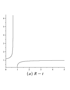
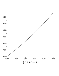
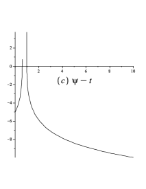
Figure 1: (a) plot of scale factor $R$ in terms of cosmic time $t$ for the small radius of Hagedorn regime. (b) plot of Hubble parameter $H$ in terms of cosmic time $t$ for the small radius of Hagedorn regime. (c) plot of dilaton field $\psi$ in terms of cosmic time $t$ for the small radius of Hagedorn regime. We take initial values $\mu_{0}=0.001$, $\dot{\mu}_{0}=0.2$ and $\psi_{0}=-5$ from the Ref. [16].

Then we must evaluate the interaction rate per string, $\Gamma$. We will calculate interaction rate for two cases, short and large strings. Before that we should note that in the Ref. [15] string interaction rates in the string gas cosmology has been studied. We use the idea of Ref. [14] to divide interaction rates to short and long string cases, then we use corresponding values of $\omega(\varepsilon)$ and $\Omega(E)$ for the closed string case, which introduced in the section 2. In that case one can find $\Gamma_{short}\sim e^{\psi}[-1+\ln{E}]$ and $\Gamma_{long}\sim\frac{-1+\ln{E}}{2\ln{E}}E^{2}e^{\psi}$. Now thermal equilibrium requires that the interaction rate per string $\Gamma$ to be larger than the expansion rate $H$: $\Gamma\geq H$. This condition satisfied for short strings if $\ln{E}\geq C$. In another word if $\ln{E}\geq\dot{\mu}_{0}e^{-\psi_{0}}+1$ there is thermal equilibrium for short strings. For the initial values of field which given by Ref. [16] there is not thermal equilibrium. In another word, with $E\geq e^{29}$ there is thermal equilibrium for short strings. It means that, very large amount of energy requested to have thermal equilibrium in presence of short strings.
Also there is thermal equilibrium for long string if $\frac{E^{2}}{2}(1-(\ln{E})^{-1})\geq C$. The initial values of fields say that there are thermal equilibrium for long strings in small radius of Hagedorn regime.
There is important discussion about above results. It is known that thermodynamics should be used to determine whether the system is dominated by short or long strings. We just written possible conditions to have thermal equilibrium in presence of the short and long strings.

3.2 large radius

In the section 2 we have shown that for large radius $P_{d}=P_{d-9}$. Now we denote pressures with $P$ and rewrite equations of motion (8) as following,

$${\dot{\psi}^{2}}-9\dot{\mu}^{2} = Ee^{\psi},$$

$$\ddot{\mu}-\dot{\mu}\dot{\psi} = \frac{1}{2}Pe^{\psi},$$

$$\ddot{\psi}-9{\dot{\mu}^{2}} = \frac{1}{2}Ee^{\psi}.$$ (14)

It is clear that when the pressures are not ignorable the energy-momentum conservation requires both $E$ and $P$ to depend on time. In the case of zero-pressure energy-momentum conservation imposes the energy $E$ to be a constant. The Ref. [20] pointed out these discusses solutions with non-vanishing pressure, and showed that it is very difficult to obtain explicit solutions when pressures are very large. Now, we suppose that pressure $P$ is approximately constant and one can obtain solutions of equation (14) as following expressions,

$$\psi = -\ln{[\frac{E}{4}t^{2}-C_{1}t+C_{2}]},$$

$$\mu = \frac{1}{3}\ln{\left[\frac{E(\frac{E}{2}+\frac{3P}{8})t^{2}-C_{1}(2E+\frac{3P}{2})t+2C_{1}^{2}+\frac{3C_{2}P}{2}}{E(\frac{E}{2}-\frac{3P}{8})t^{2}-C_{1}(2E-\frac{3P}{2})t+2C_{1}^{2}-\frac{3C_{2}P}{2}}\right]},$$ (15)

where $C_{2}=e^{-\psi_{0}}$ and $C_{1}=\sqrt{\frac{3PC_{2}}{4}\frac{e^{3\mu_{0}}+1}{e^{3\mu_{0}}-1}}$. Therefore one can find Hubble parameter as,

$$H=-\frac{P}{2Et-4C_{1}},$$ (16)

so, the initial Hubble rate is $H_{0}=\frac{P}{4C_{1}}$. We draw the plots of functions $R=e^{\mu}$, $H=\dot{\mu}$ and $\psi$ for $C_{1}=27238.6522$, $C_{2}=148.413159$ and $P=10^{4}$ in figure 2 (We take initial values of fields from Ref. [16]). As we can see from Fig.s 2 (a) and (b) there is Jeans instability for the case of closed strings which is agree with Ref. [14].

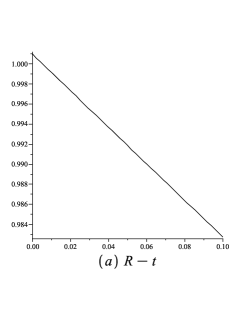
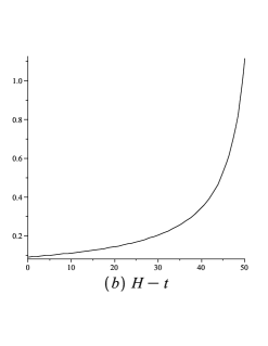
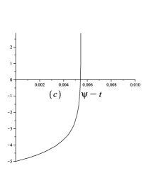
Figure 2: (a) plot of scale factor $R$ in terms of cosmic time $t$ for the large radius of Hagedorn regime. (b) plot of Hubble parameter $H$ in terms of cosmic time $t$ for the large radius of Hagedorn regime. (c) plot of dilaton field $\psi$ in terms of cosmic time $t$ for the large radius of Hagedorn regime. We take initial values $\mu_{0}=0.001$, $\dot{\mu}_{0}=0.2$ and $\psi_{0}=-5$ from the Ref. [16].

In order to obtain thermal equilibrium conditions (which is a relation between $P$ and $E$), we must have $8(2C_{1}-Et)\ln{E}\geq(Et^{2}-4C_{1}+4C_{2})P$ for short strings, and also have $4E^{2}(1-\frac{1}{\ln{E}})(2C_{1}-Et)\geq(Et^{2}-4C_{1}+4C_{2})P$ for long strings.
Now, let us rewrite equations (14) as the following form,

$${\psi}^{\prime\prime} = -\frac{1}{2}Ee^{-\psi},$$

$$\mu^{\prime\prime} = \frac{1}{2}Pe^{-\psi},$$

$${\psi^{\prime}}^{2}-9{\mu^{\prime}}^{2} = Ee^{-\psi},$$ (17)

where we used conformal time $\eta$ given by $e^{-\psi}d\eta=dt$. In the equations (14) derivatives are with respect to $\eta$. The first two equations of (14) give the following relation between $\psi$ and $\mu$,,

$$\psi=-\frac{E}{P}\mu+(\frac{E}{P}\mu_{0}^{\prime}+\psi_{0}^{\prime})\eta+\frac{E}{P}\mu_{0}+\psi_{0}.$$ (18)

Under assumption of $E\ll P$ and using relations (17) and (18), one can find following expressions for $\psi$ and $\mu$ in terms of conformal time $\eta$,

$$\psi = -\frac{E}{2{\psi_{0}^{\prime}}^{2}}e^{-\psi_{0}}(e^{-\psi_{0}^{\prime}\eta}-1)+(\psi_{0}^{\prime}-\frac{E}{2\psi_{0}^{\prime}}e^{-\psi_{0}})\eta+\psi_{0},$$

$$\mu = +\frac{P}{2{\psi_{0}^{\prime}}^{2}}e^{-\psi_{0}}(e^{-\psi_{0}^{\prime}\eta}-1)+(\mu_{0}^{\prime}+\frac{P}{2\psi_{0}^{\prime}}e^{-\psi_{0}})\eta+\mu_{0}.$$ (19)

So, we find Hubble parameter as $H=\dot{\mu}=\mu^{\prime}\exp{\psi}$. In figure 3 we give plots of $R$, $H$ and $\psi$ in terms of conformal time $\eta$, with initial values of $\psi_{0}=-5$, $\psi_{0}^{\prime}=395.403377$, $\mu_{0}=0.001$, $\mu_{0}^{\prime}=29.6826318$, $E=1000$ and $P=10^{4}$ [16]. In contrast with previous case, which is expressed in terms of cosmic time, we can see from Fig.s 3 (a) and (b) that, there is Jeans stability in conformal time for closed strings.

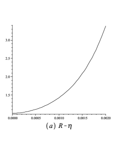
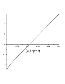
Figure 3: (a) plot of scale factor $R$ in terms of conformal time $\eta$ for the large radius of Hagedorn regime. (b) plot of Hubble parameter $H$ in terms of conformal time $\eta$ for the large radius of Hagedorn regime. (c) plot of dilaton field $\psi$ in terms of conformal time $\eta$ for the large radius of Hagedorn regime.We take initial values $\mu_{0}=0.001$, $\dot{\mu}_{0}=0.2$ and $\psi_{0}=-5$ from the Ref. [16].

Comparing the Hubble parameter with the interaction rate for short and long string yields us to following thermal equilibrium conditions for short and long strings respectively,

$$\ln E\geq-\frac{P}{2\psi_{0}^{\prime}}e^{-\psi_{0}}(e^{-\psi_{0}^{\prime}\eta}-1)+\mu_{0}^{\prime},$$ (20)

and

$$\frac{E^{2}}{2}(1-\frac{1}{\ln{E}})\geq-\frac{P}{2\psi_{0}^{\prime}}e^{-\psi_{0}}(e^{-\psi_{0}^{\prime}\eta}-1)+\mu_{0}^{\prime}.$$ (21)

In figure 4 we describe thermal equilibrium conditions for short and long strings. In the Fig. 4 (a) curve of $\ln{E}$ drawn for $E\sim 10^{13}$ and in Fig. 4 (b) curve of $\frac{E^{2}}{2}(1-\frac{1}{\ln{E}})$ drawn for small energy ($E\in[4,20]$). On the other hand in Fig. 4 (c) curve of right hand sides of equations (21) and (22) represented which have linear behavior for early time. From Fig.s 4 (a) and 4 (c) one can find that there is thermal equilibrium in the early universe if and only if the value of energy became very large ($E\sim 5\times 10^{13}$). Therefore under consideration of initial values of Ref. [16] ($E\in[500,5000]$) there is not thermal equilibrium for short strings. On the other hand, by comparing Fig.s 4 (b) and 4 (c), one can see that thermal equilibrium condition in presence of long strings satisfied at the early universe with low energy ($E\sim 10$). Again, for initial value where $E\in[500,5000]$ there is not thermal equilibrium for short strings in Hagedorn regime.

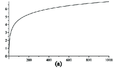
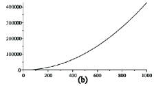
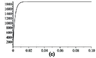
Figure 4: (a) plot of $\ln E$ for short strings in Hagedorn regime. (b) plot of $\frac{E^{2}}{2}(1-\frac{1}{\ln{E}})$ for long strings in Hagedorn regime.(c) plot of $\mu_{0}^{\prime}-\frac{P}{2\psi_{0}^{\prime}}e^{-\psi_{0}}(e^{-\psi_{0}^{\prime}\eta}-1)$ in Hagedorn regime. We take initial values $\psi_{0}=-5$, $\psi_{0}^{\prime}=395.403377$ and $\mu_{0}^{\prime}=29.6826318$ [16].

4 Dilaton gravity and pure radiation regime

In this section, again we consider action (7) and equations of motion (8). We assume that $d$ dimensions ($R$) start to expand while $9-d$ dimensions ($r$) remain small [16]. In this procedure the temperature reach below the Hagedorn regime where dynamics of the system described by massless states which is called radiation regime. We would like to solve the dilaton - gravity equations (8) and dedermine all fields. Then by specifying Hubble parameter and interaction rate we are able to study thermal equilibrium of the system. As we can see from Ref. [16], $P_{rad}^{(d)}=\frac{E_{rad}^{(d)}}{d}$ and $P_{rad}^{(9-d)}=0$. So, one can write the dilaton - gravity equations (8) as the following,

$$\ddot{\psi} = \frac{d}{2}\dot{\mu}^{2}+\frac{9-d}{2}{\dot{\nu}^{2}}+\frac{1}{2}\dot{\psi}^{2},$$

$$\ddot{\mu} = \dot{\mu}\dot{\psi}+\frac{1}{2}P_{rad}^{(d)}e^{\psi},$$

$$\ddot{\nu} = \dot{\nu}\dot{\psi}$$

$$\dot{\psi}^{2} = d\dot{\mu}^{2}+(9-d)\dot{\nu}^{2}+E_{rad}^{(d)}e^{\psi}.$$ (22)

The third equation of (22) gives,

$$\dot{\nu}=Ce^{\psi},$$ (23)

where $C=\dot{\nu}_{0}e^{-\psi_{0}}$, in terms of initial values $\dot{\nu}_{0}$ and $\psi_{0}$. From condition (23) we see that, if $\dot{\nu}_{0}$ is negative then, the expansion rate for the $9-d$ small dimensions is always negative and vis versa. If $P_{rad}^{(d)}$ in the second relation of (22) vanishes, then the evolution of the large dimensions is similar to the small dimensions.
From equations (23) it is easy to find the following equations,

$$\psi = -\ln{[\frac{E_{rad}^{(d)}}{4}t^{2}-C_{1}t+C_{2}]},$$

$$\mu = \frac{1}{2\sqrt{d}}\left[1-\frac{(9-d)C^{2}}{C_{1}^{2}-E_{rad}^{(d)}C_{2}}\right]^{\frac{1}{2}}\ln{\left[\frac{\frac{E_{rad}^{(d)}}{2}t-C_{1}-\sqrt{C_{1}^{2}-E_{rad}^{(d)}C_{2}}}{\frac{E_{rad}^{(d)}}{2}t-C_{1}+\sqrt{C_{1}^{2}-E_{rad}^{(d)}C_{2}}}\right]}+\mu_{0},$$

$$\nu = \frac{C}{\sqrt{C_{1}^{2}-E_{rad}^{(d)}C_{2}}}\ln{\left[\frac{\frac{E_{rad}^{(d)}}{2}t-C_{1}-\sqrt{C_{1}^{2}-E_{rad}^{(d)}C_{2}}}{\frac{E_{rad}^{(d)}}{2}t-C_{1}+\sqrt{C_{1}^{2}-E_{rad}^{(d)}C_{2}}}\right]}+\nu_{0},$$ (24)

where $C_{1}=\sqrt{\frac{3P_{rad}^{(d)}}{4e^{\psi_{0}}}\frac{e^{3\mu_{0}}+1}{e^{3\mu_{0}}-1}}$ and $C_{2}=e^{-\psi_{0}}$. In this case there are two scale factors corresponding to large and small dimensions as,

$$R = \left[\frac{\frac{E_{rad}^{(d)}}{2}t-C_{1}-\sqrt{C_{1}^{2}-E_{rad}^{(d)}C_{2}}}{\frac{E_{rad}^{(d)}}{2}t-C_{1}+\sqrt{C_{1}^{2}-E_{rad}^{(d)}C_{2}}}\right]^{M}e^{\mu_{0}},$$

$$r = \left[\frac{\frac{E_{rad}^{(d)}}{2}t-C_{1}-\sqrt{C_{1}^{2}-E_{rad}^{(d)}C_{2}}}{\frac{E_{rad}^{(d)}}{2}t-C_{1}+\sqrt{C_{1}^{2}-E_{rad}^{(d)}C_{2}}}\right]^{N}e^{\nu_{0}},$$ (25)

where $M=\frac{1}{2\sqrt{d}}\left[1-\frac{(9-d)C^{2}}{C_{1}^{2}-E_{rad}^{(d)}C_{2}}\right]^{\frac{1}{2}}$ and $N=\frac{C}{\sqrt{C_{1}^{2}-E_{rad}^{(d)}C_{2}}}$.

Also there are two Hubble expansion parameter corresponding to the $\mu$ and $\nu$ as the following,

$$H_{\mu}=\dot{\mu} = \sqrt{\frac{C_{1}^{2}-E_{rad}^{(d)}C_{2}-(9-d)C^{2}}{d}}\frac{2}{E_{rad}^{(d)}t^{2}-4C_{1}t+4C_{2}},$$

$$H_{\nu}=\dot{\nu} = \frac{4C}{E_{rad}^{(d)}t^{2}-4C_{1}t+4C_{2}}.$$ (26)

As we know our universe have three extended space dimensions, thus it is interesting to consider $d=3$. Therefore we find four conditions for thermal equilibrium (We take initial values of fields as $\dot{\mu}_{0}=1$, $\mu_{0}=4$, $\dot{\nu}_{0}=-0.01$, $\nu_{0}=0$ and $\psi_{0}=-16$ from Ref. [16]).
The first case is short strings in large dimensions. In this case thermal equilibrium condition written as,

$$2(\ln E_{rad}^{(d)})^{2}+\frac{1}{6}(E_{rad}^{(d)}-\frac{E_{rad}^{(d)}}{4}\frac{e^{3\mu_{0}}+1}{e^{3\mu_{0}}-1})e^{-\psi_{0}}\geq-\dot{\nu}_{0}^{2}e^{-2\psi_{0}}.$$ (27)

The second case is long strings in large dimensions. In this case thermal equilibrium condition given by,

$$3(E_{rad}^{(d)})^{4}\frac{1+(\ln E_{rad}^{(d)})^{2}-2\ln E_{rad}^{(d)}}{(\ln E_{rad}^{(d)})^{2}}+(E_{rad}^{(d)}-\frac{E_{rad}^{(d)}}{4}\frac{e^{3\mu_{0}}+1}{e^{3\mu_{0}}-1})e^{-\psi_{0}}\geq-6\dot{\nu}_{0}^{2}e^{-2\psi_{0}}.$$ (28)

The third case is short strings in small dimensions. In this case thermal equilibrium condition expressed as following,

$$\ln E_{rad}^{(d)}\geq\dot{\nu}_{0}^{2}e^{-2\psi_{0}}.$$ (29)

Finally the last case is long strings in small dimensions. In this case thermal equilibrium condition read as,

$$(E_{rad}^{(d)})^{2}(\frac{1}{2}-\frac{1}{2\ln E_{rad}^{(d)}})\geq\dot{\nu}_{0}^{2}e^{-2\psi_{0}}.$$ (30)

It is easy to check that, for above initial values, there is thermal equilibrium for given any positive energy. Only condition which break thermal equilibrium in this regime is very large negative energy ($E\sim e^{-\psi_{0}}$).

5 Conclusion

In this article thermal equilibrium of the early universe in string gas cosmology (BV scenario) dominated by closed strings investigated. In order to find thermal equilibrium, first we obtained closed string entropy similar to method of Ref. [14]. Then we obtained thermal equilibrium conditions in the Hagedorn and radiation regimes. We assumed that, range of the energy must be in the interval $500\leq E\leq 5000$ [16]. We found that in this range there is not thermal equilibrium for both short and long strings in small radius of Hagedorn regime. We have shown values of energy which thermal equilibrium satisfied. We saw that for short strings in small radius of the Hagedorn regime the total energy must be very large to have thermal equilibrium, but for long strings in small radius of the Hagedorn regime the small energy is sufficient to have thermal equilibrium. On the other hand in the large radius of the Hagedorn regime (in presence of pressure) we obtained thermal equilibrium conditions for short and long strings. In this case we have shown that there is possibility of avoiding Jeans instability by using conformal time, while for cosmic time, there is Jeans instability. Also in the case of short and long strings in the large radius of the Hagedorn regime, by using the conformal time, we found that there isn’t thermal equilibrium for the given energy in the range of $500\leq E\leq 5000$. Finally we considered another regime which is called radiation regime. In this regime, some of dimensions start to expand, which denoted by $d$, and the rest remain small. We found that there is thermal equilibrium for the case of $d=3$ in short and long strings in large and small dimensions.

References

- [1] R. Brandenberger and C. Vafa Nucl. Phys. B 316 (1989) 391
- [2] A. A. Tseytlin and C. Vafa, Nucl. Phys. B 372 (1992) 443 [arXiv:hep-th/9109048].
- [3] A. A. Tseytlin, Class. Quant. Grav. 9 (1992) 979 [arXiv:hep-th/9112004].
- [4] M. A. Osorio and M. A. Vazquez-Mozo, Mod. Phys. Lett. A 8 (1993) 3111 [arXiv:hep-th/9305137]; Mod. Phys. Lett. A 8 (1993) 3215 [arXiv:hep-th/9305138].
- [5] G. B. Cleaver and P. J. Rosenthal, Nucl. Phys. B 457 (1995) 621 [arXiv:hep-th/9402088].
- [6] M. Sakellariadou, Nucl. Phys. B 468 (1996) 319 [arXiv:hep-th/9511075].
- [7] S. Alexander, R. H. Brandenberger and D. Easson, Phys. Rev. D 62 (2000) 103509 [arXiv:hep-th/0005212].
- [8] R. Brandenberger, D. A. Easson and D. Kimberly, Nucl. Phys. B 623 (2002) 421 [arXiv:hep-th/0109165].
- [9] D. A. Easson, Int.J.Mod.Phys. A18 (2003) 4295-4314 [arXiv:hep-th/0110225].
- [10] R. Easther, B. R. Greene and M. G. Jackson, Phys. Rev. D 66 (2002) 023502 [arXiv:hep-th/0204099].
- [11] S. Watson and R. H. Brandenberger, Phys.Rev. D67 (2003) 043510 [arXiv:hep-th/0207168].
- [12] R. Easther, B. R. Greene, M. G. Jackson and D. Kabat, Phys.Rev.D67(2003)123501 [arXiv:hep-th/0211124].
- [13] Y. Leblanc, Phys. Rev. D 38 (1988) 3087.
- [14] Ayse Arslanargin, Ali Kaya [arXiv:0901.4608].
- [15] Rebecca Danos, Andrew R. Frey, Anupam Mazumdar, Phys.Rev. D70 (2004) 106010 [arXiv:hep-th/0409162]
- [16] Bruce A. Bassett, Monica Borunda, Marco Serone, Shinji Tsujikawa, Phys.Rev. D67 (2003) 123506 [arXiv:hep-th/0301180].
- [17] R. Hagedorn, suppl. Nuovo Cimento 3 (1965)147.
- [18] D.A. Lowe, L. Thorlacius, Phys.Rev. D51 (1995) 665, [arXiv:hep-th/9408134].
- [19] M. Gasperini, G. Veneziano, Astropart.Phys. 1 (1993) 317, [arXiv:hep-th/9211021].
- [20] Dimitri Skliros, Mark Hindmarsh, Phys.Rev.D78 (2008) 063539, [arXiv:hep-th/0712.1254].