A Modified Holographic Dark Energy Model with Infrared Infinite Extra Dimension(s)

Abstract

We propose a modified holographic dark energy (MHDE) model with the Hubble scale as the infrared (IR) cutoff. Introducing the infinite extra dimension(s) at very large distance scale, we consider the black hole mass in higher dimensions as the ultraviolet cutoff. Thus, we can probe the effects of the IR infinite extra dimension(s). As a concrete example, we consider the Dvali-Gabadadze-Porrati (DGP) model and its generalization. We find that the DGP model is dual to the MHDE model in five dimensions, and the $\Lambda$CDM model is dual to the MHDE model in six dimensions. Fitting the MHDE model to the observational data, we obtain that $\Omega_{m0}=0.269^{+0.030}_{-0.027}$, $\Omega_{k0}=0.003^{+0.011}_{-0.012}$, and the number of the spatial dimensions is $N=4.78^{+0.68}_{-0.44}$. The best fit value of $N$ implies that there might exist two IR infinite extra dimensions.

I Introduction

From the cosmological observations such as Type Ia supernova (SN Ia) Riess , cosmic microwave background (CMB) spergel , and large scale structure (LSS) Tegmark , there are strong evidences for dark energy (DE) which drives the accelerated expansion of the Universe. The most naive DE candidate is the cosmological constant (CC) introduced by Einstein. Although CC is consistent with the cosmological observations, there exists a fine-tuning problem Weinberg : CC ($(2.3\times 10^{-3}~{}{\rm eV})^{4}$) is extremely small comparing to the known energy scales such as the reduced Planck scale $M_{\rm Pl}\equiv 1/\sqrt{8\pi G}$ (about $2.4\times 10^{19}~{}{\rm GeV}$) in general relativity and the electroweak scale (about $91~{}{\rm GeV}$) in particle physics, and we do not have any symmetry which can protect the tiny CC against quantum corrections (supersymmetry must be broken above the electroweak scale). This fine-tuning problem is the greatest challenge in high energy physics. Also, there is a coincident problem Weinberg : why the DE and dark matter energy densities are comparable today since their evolutions are different as the Universe expands. Therefore, cosmologists and particle physicists have proposed some other DE models, for example, quintessence quint , phantom phantom , $k$-essence k , tachyon tachyonic , quintom Feng:2004ad , hessence hessence , Chaplygin gas Chaplygin , Yang-Mills condensate YMC , etc.

The DE problem might be a problem in quantum gravity Witten . However, we do not have a complete theory of quantum gravity right now. Fortunately, an important progress in the studies of the black hole theory and string theory is the proposal of the holographic principle 't Hooft93 , which may be considered as a fundamental principle of quantum gravity and then shed some light on the DE problem. Using the effective quantum field theory, Cohen, Kaplan and Nelson suggested that the quantum zero-point energy of a system with size $L$ should not exceed the mass of a black hole with the same size, i.e., $L^{3}\rho_{\rm V}\leq LM_{\rm Pl}^{2}$, where $\rho_{\rm V}$ is the quantum zero-point energy density Cohen:1998zx . Thus, the ultraviolet (UV) cutoff scale of a system is connected to its infrared (IR) cutoff scale. Applying this idea to the whole Universe, we can consider the vacuum energy as DE with density $\rho_{\rm DE}\equiv\rho_{\rm V}$. Choosing the largest IR cutoff $L$ which saturates the inequality, we obtain the holographic DE density

$$\rho_{DE}=3c^{2}M_{\rm Pl}^{2}L^{-2}~{},$$ (1)

where $c$ is an unknown constant due to the theoretical uncertainties and can only be determined by observations. Interestingly, taking $L$ as the size of the current Universe which is the Hubble radius $H^{-1}$, one finds that the DE density is close to the observed value. However, Hsu Hsu pointed out that this yields a wrong equation of state for DE.

To solve this problem, Li Li chose the future event horizon of the Universe as the IR cutoff, and found that the model is a viable DE model. However, there exists an obvious draw back concerning causality: the event horizon is a global concept of space-time, and the existence of event horizon depends on the future evolution of the Universe, i.e., the event horizon exists if and only if the Universe is accelerating. So, the original holographic DE model has presumed the existence of accelerated expansion. To avoid the causality problem, Cai proposed the agegraphic DE model in which the age of the Universe can be chosen as the IR cutoff Cai . A new version of this model, which replaces the age of the Universe by the conformal age of the Universe, was suggested as well Wei . Moreover, Gao, Wu, Chen, and Shen proposed the holographic Ricci DE model where the average radius of the Ricci scalar curvature is chosen as the IR cutoff Gao . The phenomenological consequences of these models have been studied extensively refHDE ; refADE ; refRDE ; Li:2009bn .

In this Letter, to obtain the accelerating Universe and solve the causality problem, we propose a modified holographic DE (MHDE) model with the Hubble scale as the IR cutoff, and the UV and IR connection is modified by using the black hole mass in higher dimensions. As a concrete example, we consider the Dvali-Gabadadze-Porrati (DGP) models which have infinite extra dimension(s) dgp ; dg . The characteristic distance scale in such theories is called the crossover scale $r_{c}$ (for definitions, please see Section II.). At the distances that are smaller than $r_{c}$, we observe four-dimensional gravity. While at the distances larger than $r_{c}$, we observe higher-dimensional gravity. So at the IR energy scale which is smaller than $r_{c}^{-1}$ (or say at the distance larger than $r_{c}$), we need to consider the effect of extra dimensions. In particular, the mass of the higher-dimensional black hole is different from that of the four-dimensional one. Therefore, the UV cutoff scale in the MHDE model is different from that in the original holographic DE model. Moreover, our model provides a way to probe the IR infinite extra dimensions: the DGP model is dual to the MHDE model in five dimensions, and the $\Lambda$CDM model is dual to the MHDE model in six dimensions. Interestingly, with the Hubble scale as the IR cutoff scale, we can not only obtain the observed DE density with correct equation of state, but also avoid the causality problem. The best fit value indicates that there might exist two IR infinite extra dimensions.

This Letter is organized as follows. We present our model in Section II. And we discuss the observational constraints in Section III. Our conclusion is in Section IV.

II The model

First, let us briefly review the DGP model and its generalization dgp ; dg . The theory is a brane-world model which is embedded in a space-time with (asymptotically) flat infinite $n$ extra space dimensions. All the standard model (SM) particles are localized on the D3-branes, and the corresponding cut-off scale on the observable D3-branes can be the grand unification scale or higher. Also, the gravity spreads over the whole $4+n$ space-time dimensions. Thus, the action is

$$S~{}=~{}{{M_{*}^{2+n}}\over 2}\int d^{4}xd^{n}y{\sqrt{G}}{\cal R}+\int d^{4}x{\sqrt{g}}\left(T_{0}+{{M^{2}_{\rm Pl}}\over 2}R+{\cal L}_{\rm SM}\right)~{},~{}\,$$ (2)

where $x^{\mu}$ and $y^{i}$ are respectively the coordinates for the Minkowski space-time and the extra space dimensions, $G=|{\rm det}(G_{AB})|$ and $G_{AB}$ is the metric for the whole space-time, $g=|{\rm det}(g_{\mu\nu})|$ and $g_{\mu\nu}$ is the reduced metric on the D3-branes, $M_{*}$ is the high-dimensional Planck scale, $T_{0}$ is the brane tension, and ${\cal L}_{\rm SM}$ is the SM Lagrangian dgp ; dg . The characteristic distance scale in such theories is called the crossover scale. For five-dimensional space-time with $n=1$, the crossover scale is dgp

$$r_{c}~{}\sim~{}{{M_{\rm Pl}^{2}}\over{M_{*}^{3}}}~{}.~{}\,$$ (3)

And for six- or higher-dimensional space-time with zero tension branes, i.e., $n\geq 2$, the crossover scale is Dvali:2001ae

$$r_{c}~{}\sim~{}{{M_{\rm Pl}}\over{M_{*}^{2}}}~{}.~{}\,$$ (4)

Interestingly, at distance smaller than $r_{c}$, i.e., $r<r_{c}$, we observe the four-dimensional gravity, while at distance $r>r_{c}$, we indeed observe high-dimensional gravity. Moreover, from the data on sub-millimeter gravity measurements adel and the accelerator, astrophysical and cosmological data Dvali:2001gm , the lower bound on the value of $M_{*}$ is $M_{*}\geq 10^{-3}~{}{\rm eV}$. Also, from the solar system measurements of Newton’s law, one obtains the upper bound on $M_{*}$: $M_{*}\leq 10^{12}~{}{\rm eV}$ for five-dimensional space-time, and $M_{*}\leq 10^{4}~{}{\rm eV}$ for six- and higher-dimensional space-time Dvali:2001ae ; Dick:2001np .

The idea of holography may be used to solve the CC problem Cohen:1998zx ; lvdark . Cohen, Kaplan and Nelson proposed that for any state with energy $E$ in the Hilbert space, the corresponding Schwarzschild radius $R_{s}\sim E$ is less than the IR cutoff $L$ Cohen:1998zx . Under this assumption, a relationship between the UV cutoff $\rho_{D}^{1/4}$ and the IR cutoff is derived, i.e., $L^{3}\rho_{d}\sim L$ Cohen:1998zx . Here the relationship $M\sim R_{s}$ between the mass and the horizon of the Schwarzschild black hole in four dimensions is used. In $N+1$ dimensions with $N\equiv n+3$, the mass of the Schwarzschild black hole is myers

$$M=\frac{(N-1)\Omega_{N-1}}{16\pi G_{N}}r^{N-2}_{H}~{},~{}\,$$ (5)

where $8\pi G_{N}\equiv M_{*}^{1-N}$. If we can see the effect of extra dimensions, then we have the relation

$$L^{3}\rho_{d}\sim\frac{(N-1)\Omega_{N-1}}{16\pi G_{N}}L^{N-2},$$ (6)

and the DE density

$$\rho_{d}=\frac{d(N-1)\Omega_{N-1}}{16\pi G_{N}}L^{N-5},$$ (7)

where $d$ is an unknown constant accounting for theoretical uncertainties. If we choose the Hubble horizon as the IR cutoff, then we get the MHDE density

$$\rho_{d}=\frac{d(N-1)\Omega_{N-1}}{16\pi G_{N}}H^{5-N}.$$ (8)

The mass of the Schwarzschild black hole is

$$M=\frac{(N-1)\Omega_{N-1}}{2}M_{*}^{N-1}r_{H}^{N-2}~{}.~{}\,$$ (9)

Thus, the high-dimensional black hole mass can be much higher than the Planck scale in our scenarios. However, to compare with particle physics theory, we consider the Lagrangian density. In our models, we have the dark energy density as follows

$$\rho_{d}=\frac{d(N-1)\Omega_{N-1}}{2}M_{*}^{N-1}L^{N-5}.$$ (10)

Thus, for the model with one or two extra dimensions, the dark energy density is proportional to $M_{*}^{3}L^{-1}$ and $M_{*}^{4}$, respectively. Thus, they are consistent with particle physics theory. However, for the models with three or more extra dimensions, the dark energy density is proportional to $M_{*}^{N-1}L^{N-5}$ with $N\geq 6$, thus, these models may have pretty large dark energy density, which is not consistent with particle physics. Therefore, we only consider one or two extra dimensions, i.e., the space-time dimensions are five and six, respectively. In particular, for five-dimensional and six-dimensional space-time, we obtain the observed DE density for $M_{*}\sim 10^{7}~{}{\rm eV}$ and $M_{*}\sim 10^{-3}~{}{\rm eV}$, respectively. Now the Friedmann equation becomes

$$H^{2}+\frac{k}{a^{2}}=\frac{8\pi G}{3}(\rho_{m}+\rho_{r}+\rho_{d}),$$ (11)

where the matter energy density $\rho_{m}=\rho_{m0}(a_{0}/a)^{3}$ and the radiation energy density $\rho_{r}=\rho_{r0}(a_{0}/a)^{4}$. Substituting Eq. (10) into Eq. (11), we get

$$\left(\frac{H}{H_{0}}\right)^{2}-(1-\Omega_{m0}-\Omega_{k0}-\Omega_{r0})\left(\frac{H}{H_{0}}\right)^{5-N}=\Omega_{m0}(1+z)^{3}+\Omega_{r0}(1+z)^{4}+\Omega_{k0}(1+z)^{2}.$$ (12)

This is the same as the $\alpha$ dark energy model proposed by Dvali and Turner in Ref. turner where $\alpha=5-N$. The crossover scale in this model is

$$r_{c}\sim\frac{M_{\rm Pl}^{2/(N-3)}}{M_{*}^{(N-1)/(N-3)}}~{}.~{}\,$$ (13)

In turner , the model is proposed as the modification to the Friedmann equation motivated by extra dimensions, and it was found that $\alpha\lesssim 1$ to be consistent with astronomical observations. Here we use the holographic idea to derive the above Friedmann equation and take the model as a dark energy model. We also connect the holographic idea with the effect of IR infinite extra dimensions. Furthermore, the parameter $\alpha$ has the physical meaning of the number of the spatial dimensions. If $N=4$, i.e. , with one extra dimension, we recover the DGP model for the flat case. So the DGP model may be interpreted as the holographic dark energy model with the Hubble scale as the IR cutoff. When $N=5$, i.e., with two extra dimensions, we recover the standard $\Lambda$CDM model. In other words, the cosmological constant is a special case of our model, and it may be interpreted as the effect of two extra dimensions. In our model, we choose the Hubble scale as the IR cutoff, so the problem of circular reasoning is avoided. In addition, the choice of the Hubble scale as the IR cutoff is more natural than other choices.

Combining the Friedmann equation (11) with the energy conservation, we get the equation of state parameter $w_{d}$ for the MHDE

$$w_{d}=-1+\frac{2\alpha(1-\Omega_{d})}{3(2-\alpha\Omega_{d})}+\frac{\alpha(\Omega_{m}+2\Omega_{r})}{3(2-\alpha\Omega_{d})}.$$ (14)

So $w_{d}$ changes from $-1+2\alpha/3$ during the radiation dominated era to $-1+\alpha/2$ during the matter dominated era. The deceleration parameter $q=-\ddot{a}/(aH^{2})$ is

$$q=-1+\frac{2\Omega_{k}+3\Omega_{m}+4\Omega_{r}}{2-\alpha\Omega_{d}}.$$ (15)

Using the Friedmann equation $\Omega_{m}+\Omega_{r}+\Omega_{k}+\Omega_{d}=1$ and $q=0$, we obtain at the transition redshift $z_{t}$

$$(N-3)\Omega_{k}(z_{t})+(N-2)\Omega_{m}(z_{t})+(N-1)\Omega_{r}(z_{t})=N-3.$$ (16)

Since the transition from deceleration to acceleration happened very recently, we can ignore the contribution due to the radiation, and then we have

$$(N-3)\Omega_{k0}(1+z_{t})^{2}+(N-2)\Omega_{m0}(1+z_{t})^{3}=(N-3)(H/H_{0})^{2}.$$ (17)

III Observational constraints

Now we use the observational data to fit the MHDE model. The parameters in the model are determined by minimizing $\chi^{2}=\chi^{2}_{sn}+\chi^{2}_{bao}+\chi^{2}_{cmb}+\chi^{2}_{h}$. For the SN Ia data, we use the Constitution compilation of 397 SN Ia consta . The Constitution sample adds 185 CfA3 SN Ia data to the Union sample union . The addition of CfA3 sample increases the number of nearby SN Ia by a factor of roughly $2.6-2.9$ and reduces the statistical uncertainties. The Union compilation has 57 nearby SN Ia and 250 high-$z$ SN Ia. It includes the Supernova Legacy Survey astier and the ESSENCE Survey riess ; essence , the older observed SN Ia data, and the extended data set of distant SN Ia observed with the Hubble space telescope. To fit the SN Ia data, we define

$$\chi^{2}_{sn}=\sum_{i=1}^{307}\frac{[\mu_{obs}(z_{i})-\mu(z_{i})]^{2}}{\sigma^{2}_{i}},$$ (18)

where the extinction-corrected distance modulus $\mu(z)=5\log_{10}[d_{L}(z)/{\rm Mpc}]+25$, $\mu_{obs}$ is the observed distance modulus, $\sigma_{i}$ is the total uncertainty in the SN Ia data, and the luminosity distance is

$$d_{L}(z)=\frac{1+z}{H_{0}\sqrt{|\Omega_{k}|}}{\rm sinn}\left[\sqrt{|\Omega_{k}|}\int_{0}^{z}\frac{dz^{\prime}}{E(z^{\prime})}\right],$$ (19)

where

$$\frac{{\rm sinn}(\sqrt{|\Omega_{k}|}x)}{\sqrt{|\Omega_{k}|}}=\begin{cases}\sin(\sqrt{|\Omega_{k}|}x)/\sqrt{|\Omega_{k}|},&{\rm if}\ \Omega_{k}<0,\\ x,&{\rm if}\ \Omega_{k}=0,\\ \sinh(\sqrt{|\Omega_{k}|}x)/\sqrt{|\Omega_{k}|},&{\rm if}\ \Omega_{k}>0,\end{cases}$$ (20)

and the dimensionless Hubble parameter $E(z)=H(z)/H_{0}$. In particular, $E(z)=[\Omega_{m0}(1+z)^{3}+1-\Omega_{m0}]^{1/2}$ for the flat $\Lambda$CDM model and $E(z)=[\Omega_{m0}(1+z)^{3}+(1-\Omega_{m0})^{2}/4]^{1/2}+(1-\Omega_{m0})/2$ for the flat DGP model. We marginalized over the nuisance parameter $H_{0}$ when evaluating $\chi^{2}_{sn}$.

To use the baryon acoustic oscillation (BAO) measurement from the Sloan digital sky survey data, we define sdss6

$$\chi^{2}_{bao}=\left(\frac{r_{s}(z_{d})/D_{V}(z=0.2)-0.198}{0.0058}\right)^{2}+\left(\frac{r_{s}(z_{d})/D_{V}(z=0.35)-0.1094}{0.0033}\right)^{2},$$ (21)

where the effective distance is

$$D_{V}(z)=\left[\frac{d_{L}^{2}(z)}{(1+z)^{2}}\frac{z}{H(z)}\right]^{1/3}.$$ (22)

The redshift $z_{d}$ is fitted with the formulas hu98

$$z_{d}=\frac{1291(\Omega_{m0}h^{2})^{0.251}}{1+0.659(\Omega_{m0}h^{2})^{0.828}}[1+b_{1}(\Omega_{b}h^{2})^{b_{2}}],$$ (23)

$$b_{1}=0.313(\Omega_{m0}h^{2})^{-0.419}[1+0.607(\Omega_{m0}h^{2})^{0.674}],\quad b_{2}=0.238(\Omega_{m0}h^{2})^{0.223},$$ (24)

and the comoving sound horizon is

$$r_{s}(z)=\int_{z}^{\infty}\frac{dz^{\prime}}{c_{s}(z^{\prime})E(z^{\prime})},$$ (25)

where the sound speed $c_{s}(z)=1/\sqrt{3[1+\bar{R_{b}}/(1+z)}]$, the dimensionless Hubble constant $h=H_{0}/100$, and $\bar{R_{b}}=315000\Omega_{b}h^{2}(T_{cmb}/2.7{\rm K})^{-4}$.

To implement the Wilkinson microwave anisotropy probe 5 year (WMAP5) data, we need to add three fitting parameters $R$, $l_{a}$ and $z_{*}$, so $\chi^{2}_{cmb}=\Delta x_{i}{\rm Cov}^{-1}(x_{i},x_{j})\Delta x_{j}$, where $x_{i}=(R,\ l_{a},\ z_{*})$ denotes the three parameters for WMAP5 data, $\Delta x_{i}=x_{i}-x_{i}^{obs}$ and Cov$(x_{i},x_{j})$ is the covariance matrix for the three parameters wmap5 . The acoustic scale $l_{A}$ is

$$l_{A}=\frac{\pi d_{L}(z_{*})}{(1+z_{*})r_{s}(z_{*})},$$ (26)

where the redshift $z_{*}$ is given by hu96

$$z_{*}=1048[1+0.00124(\Omega_{b}h^{2})^{-0.738}][1+g_{1}(\Omega_{m0}h^{2})^{g_{2}}]=1090.04\pm 0.93,$$ (27)

$$g_{1}=\frac{0.0783(\Omega_{b}h^{2})^{-0.238}}{1+39.5(\Omega_{b}h^{2})^{0.763}},\quad g_{2}=\frac{0.560}{1+21.1(\Omega_{b}h^{2})^{1.81}}.$$ (28)

The shift parameter is

$$R=\frac{\sqrt{\Omega_{m0}}}{\sqrt{|\Omega_{k}|}}{\rm sinn}\left(\sqrt{|\Omega_{k}|}\int_{0}^{z_{*}}\frac{dz}{E(z)}\right)=1.710\pm 0.019.$$ (29)

Simon, Verde, and Jimenez obtained the Hubble parameter $H(z)$ at nine different redshifts from the differential ages of passively evolving galaxies hz1 . Recently, the authors in hz2 obtained $H(z=0.24)=79.69\pm 2.32$, $H(z=0.34)=83.8\pm 2.96$, and $H(z=0.43)=86.45\pm 3.27$ by taking the BAO scale as a standard ruler in the radial direction. To use these 12 $H(z)$ data, we define

$$\chi^{2}_{h}=\sum_{i=1}^{12}\frac{[H_{obs}(z_{i})-H(z_{i})]^{2}}{\sigma_{hi}^{2}},$$ (30)

where $\sigma_{hi}$ is the $1\sigma$ uncertainty in the $H(z)$ data. We also add the prior $H_{0}=74.2\pm 3.6$ km/s/Mpc given by Riess et al. riess09 . The likelihood for the parameters in the model and the nuisance parameters $\Omega_{b}h^{2}$ and $H_{0}$ ($h$) is computed using a Monte Carlo Markov chain (MCMC). The MCMC method randomly chooses values for the above parameters, evaluates $\chi^{2}$ and determines whether to accept or reject the set of parameters using the Metropolis-Hastings algorithm. The set of parameters that is accepted to the chain forms a new starting point for the next process, and the process is repeated for a sufficient number of steps until the required convergence is reached. Our MCMC code is based on the publicly available package COSMOMC cosmomc .

By fitting the flat $\Lambda$CDM model to the combined SN Ia, BAO, WMAP5 and $H(z)$ data, we find that $\chi^{2}=483.0$ and $\Omega_{m0}=0.272\pm 0.021$. If we fit the observational data to the curved $\Lambda$CDM model, we find that $\chi^{2}=482.9$, $\Omega_{m0}=0.272^{+0.026}_{-0.024}$ and $\Omega_{k0}=0.001_{-0.009}^{+0.010}$. The contour plots and the probability distributions are shown in Figs. 1 and 2. By fitting the observational data to the flat MHDE model, we find that $\chi^{2}=482.5$, $\Omega_{m0}=0.269^{+0.027}_{-0.025}$ and $N=4.84^{+0.56}_{-0.40}$. The contour plots and the probability distributions are shown in Figs. 3 and 4. Substituting the best fit values $\Omega_{m0}$ and $N$ to Eq. (17), we get the transition redshift $z_{t}=0.746$. By fitting the observational data to the curved MHDE model, we find that $\chi^{2}=482.2$, $\Omega_{m0}=0.269^{+0.030}_{-0.027}$, $\Omega_{k0}=0.003^{+0.011}_{-0.012}$ and $N=4.78^{+0.68}_{-0.44}$. The contour plot and the probability distributions are shown in Figs. 5 and 6. By using the best fit values of $\Omega_{m0}$, $\Omega_{k0}$, and $N$, we find that the age of the Universe is $t_{0}=13.74$ Gyr which is consistent with the result given by WMAP5 wmap5 . Substituting the best fit values of $\Omega_{m0}$, $\Omega_{k0}$, and $N$ to Eq. (17), we get the transition redshift $z_{t}=0.739$. Since the best fit value of $\Omega_{k0}$ is very small, the spatial geometry of the Universe is almost flat, so the transition redshift $z_{t}$ is almost the same for the curved and flat cases. In other words, we can neglect the contribution due to the curvature term. By using Eqs. (14) and (15) with the best fit parameter values, we plot the evolutions of the $\Omega_{m}$ and $\Omega_{d}$, the equation of state parameter $w_{d}$, and the deceleration parameter $q$ in Fig. 7.

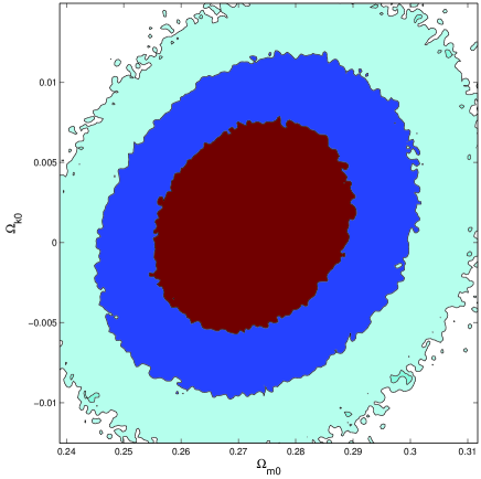
Figure 1: The marginalized contours of $\Omega_{m0}$ and $\Omega_{k0}$ in the curved $\Lambda$CDM model.

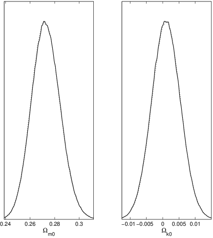
Figure 2: The probability distributions of $\Omega_{m0}$ and $\Omega_{k0}$ in the curved $\Lambda$CDM model.

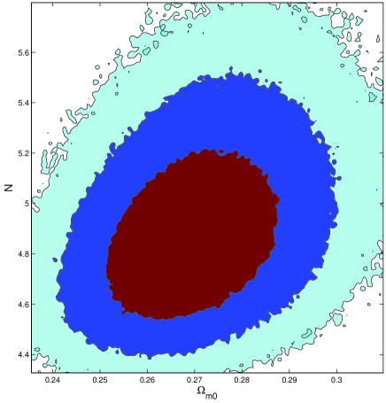
Figure 3: The marginalized contours of $\Omega_{m0}$ and $N$ in the flat MHDE model.

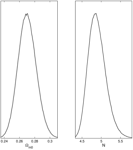
Figure 4: The probability distributions of $\Omega_{m0}$ and $N$ in the flat MHDE model.

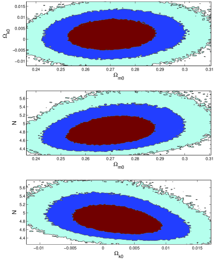
Figure 5: The marginalized contours of the parameters in the curved MHDE model.

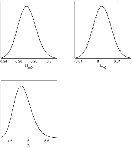
Figure 6: The probability distributions of the parameters in the curved MHDE model.

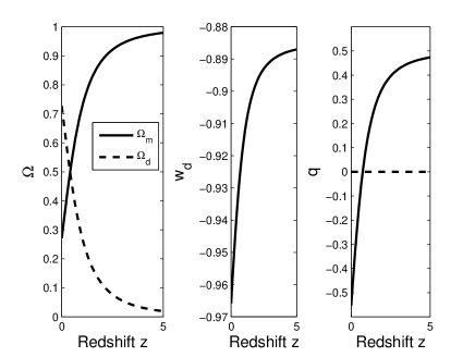
Figure 7: The left panel shows the evolutions of the matter energy density $\Omega_{m}$ and the holographic DE density $\Omega_{d}$, the middle panel shows the evolution of the holographic DE equation of state parameter $w_{d}$, and the right panel shows the evolution of the deceleration parameter $q$.

IV Conclusions

We proposed the MHDE model with the Hubble scale as the IR cutoff, and our model fits the observational data as well as that of the $\Lambda$CDM model. The black hole mass in higher dimensions is used to modify the UV and IR relation, and then to derive our model. Since we used the Hubble scale as the IR cutoff, our model avoids the problem of circular reasoning. Furthermore, our model suggests a way probing IR infinite extra dimensions since the DGP model and the $\Lambda$CDM model are special cases of our model. In particular, the DGP model is dual to the MHDE model in five dimensions, and the $\Lambda$CDM model is dual to the MHDE in six dimensions. In other words, the effect of one extra dimension is manifested as the DGP model, i.e., the effect of five-dimensional gravity at large distance can be seen as DE in four dimensions. Also, the effect of six-dimensional gravity at large distance can be considered as the CC in four dimensions. Fitting the model to the combined SN Ia, BAO, WMAP5 and $H(z)$ data, we find that $\Omega_{m0}=0.269^{+0.030}_{-0.027}$, $\Omega_{k0}=0.003^{+0.011}_{-0.012}$ and $N=4.78^{+0.68}_{-0.44}$. By using the best fit values of $\Omega_{m0}$, $\Omega_{k0}$, and $N$, we find that the age of the Universe is $t_{0}=13.74$ Gyr. The best fit value of $N$ suggests that there may exist two IR infinite extra dimensions.

- (1) A.G. Riess et al., AJ. 116, 1009 (1998); S. Perlmutter et al., ApJ 517, 565 (1999); J. L. Tonry et al., ApJ 594, 1 (2003); R.A. Knop et al., ApJ 598, 102 (2003); A.G. Riess et al., ApJ 607, 665 (2004).
- (2) C.L. Bennet et al., ApJS. 148, 1 (2003); D.N. Spergel et al., ApJS, 148, 175 (2003); D.N. Spergel et al., ApJS 170, 377 (2007); L. Page et al., ApJS 170, 335 (2007); G. Hinshaw et al., ApJS 170, 263 (2007).
- (3) M. Tegmark et al., Phys. Rev. D69, 103501 (2004); ApJ 606, 702 (2004); Phys. Rev. D74, 123507 (2006).
- (4) S. Weinberg, Rev. Mod. Phys. 61, 1 (1989); arXiv:astro-ph/0005265; V. Sahni and A.A. Starobinsky, Int. J. Mod. Phys. D 9, 373 (2000); S.M. Carroll, Living Rev.Rel. 4, 1 (2001); P.J.E. Peebles and B. Ratra, Rev. Mod. Phys. 75, 559 (2003); T. Padmanabhan, Phys. Rept. 380, 235 (2003); E. J. Copeland, M. Sami and S. Tsujikawa, Int. J. Mod. Phys. D 15, 1753 (2006).
- (5) B. Ratra and P.J.E. Peebles, Phys. Rev. D37, 3406 (1988); P.J.E. Peebles and B.Ratra, ApJ 325, L17 (1988); C. Wetterich, Nucl. Phys. B302, 668 (1988); I. Zlatev, L. Wang and P.J. Steinhardt, Phys. Rev. Lett. 82, 896 (1999).
- (6) R.R. Caldwell, Phys. Lett. B 545, 23 (2002); S.M. Carroll, M. Hoffman and M. Trodden, Phys. Rev. D68, 023509 (2003).
- (7) C. Armendariz-Picon, T. Damour and V. Mukhanov, Phys. Lett. B 458, 209 (1999) ; C. Armendariz-Picon, V. Mukhanov and P.J. Steinhardt, Phys. Rev. D63, 103510 (2001); T. Chiba, T. Okabe and M. Yamaguchi, Phys. Rev. D62, 023511 (2000).
- (8) T. Padmanabhan, Phys. Rev. D66, 021301 (2002); J.S. Bagla, H.K. Jassal, and T. Padmanabhan, Phys. Rev. D67, 063504 (2003).
- (9) B. Feng, X. L. Wang and X. M. Zhang, Phys. Lett. B 607, 35 (2005).
- (10) H. Wei, R.G. Cai, and D.F. Zeng, Class. Quant. Grav. 22, 3189 (2005); H. Wei, and R.G. Cai, Phys. Rev. D72, 123507 (2005).
- (11) A.Y. Kamenshchik, U. Moschella and V. Pasquier, Phys. Lett. B 511 265 (2001); M.C. Bento, O. Bertolami and A.A. Sen, Phys. Rev. D 66 043507 (2002); X. Zhang, F.Q. Wu and J. Zhang, JCAP 0601 003 (2006).
- (12) E. Elizalde, J. Lidsey, S. Nojiri and S.D. Odintsov, Phys. Lett. B 574 1 (2003); W. Zhao and Y. Zhang, Class. Quant. Grav. 23, 3405 (2006); Y. Zhang, T.Y. Xia, and W. Zhao, Class. Quant. Grav. 24, 3309 (2007); T.Y. Xia and Y. Zhang, Phys. Lett. B 656, 19 (2007); S. Wang, Y. Zhang and T.Y. Xia, JCAP 10 037 (2008).
- (13) E. Witten, arXiv:hep-ph/0002297.
- (14) G. ’t Hooft, arXiv:gr-qc/9310026; L. Susskind, J. Math. Phys. 36 6377 (1995).
- (15) A.G. Cohen, D.B. Kaplan and A.E. Nelson, Phys. Rev. Lett. 82, 4971 (1999).
- (16) S.D.H. Hsu, Phys. Lett. B 594 13 (2004).
- (17) M. Li, Phys. Lett. B 603 1 (2004).
- (18) R.G. Cai, Phys. Lett. B 657, 228 (2007).
- (19) H. Wei and R.G. Cai, Phys. Lett. B 660, 113 (2008).
- (20) C. Gao, F.Q. Wu, X.L. Chen and Y.G. Shen, Phys. Rev. D 79, 043511 (2009).
- (21) Q.G. Huang and M. Li, JCAP 0408, 013 (2004); Q.G. Huang and M. Li, JCAP 0503, 001 (2005); Q.G. Huang and Y.G. Gong, JCAP 0408, 006 (2004); Y.G. Gong, B. Wang and Y.Z. Zhang Phys. Rev. D 72, 043510 (2005); B. Wang, Y.G. Gong and E. Abdalla, Phys. Lett. B 624, 141 (2005); X. Zhang and F.Q. Wu, Phys. Rev. D 72, 043524 (2005); X. Zhang, Int. J. Mod. Phys. D 14, 1597 (2005); Z. Chang, F.Q. Wu and X. Zhang, Phys. Lett. B 633, 14 (2006); B. Wang, E. Abdalla and R.K. Su, Phys. Lett. B 611, 21 (2005); B. Wang, C.Y. Lin and E. Abdalla, Phys. Lett. B 637, 357 (2006); X. Zhang, Phys. Lett. B 648, 1 (2007); M.R. Setare, J. Zhang and X. Zhang, JCAP 0703, 007 (2007); J. Zhang, X. Zhang and H. Liu, Phys. Lett. B 659, 26 (2008); B. Chen, M. Li and Y. Wang, Nucl. Phys. B 774, 256 (2007); J. Zhang, X. Zhang and H.Y. Liu, Eur. Phys. J. C 52, 693 (2007); X. Zhang and F.Q. Wu, Phys. Rev. D 76, 023502 (2007); C.J. Feng, Phys. Lett. B 633, 367 (2008); Y.Z. Ma, Y. Gong and X.L. Chen, Eur. Phys. J. C 60, 303 (2009); Y.Z. Ma, Y. Gong and X.L. Chen, arXiv:0901.1215; M. Li, C. Lin and Y. Wang, JCAP 0805, 023 (2008); E.N. Saridakis, Phys. Lett. B 660, 138 (2008); JCAP 04 (2008) 020; Phys. Lett. B 661, 335 (2008); M. Li, X.D. Li, C. Lin and Y. Wang, Commun. Theor. Phys. 51, 181 (2009).
- (22) H. Wei and R.G. Cai, Phys. Lett. B 655, 1 (2007); H. Wei and R.G. Cai, Phys. Lett. B 663, 1 (2008); I.P. Neupane, Phys. Rev. D 76, 123006 (2007); M. Maziashvili, Phys. Lett. B 666, 364 (2008); J. Zhang, X. Zhang and H. Liu, Eur. Phys. J. C 54, 303 (2008); J.P. Wu, D.Z. Ma and Y. Ling, Phys. Lett. B 663, 152 (2008); H. Wei and R.G. Cai, Eur. Phys. J. C 59, 99 (2009); J. Cui, L. Zhang, J. Zhang and X. Zhang, arXiv: 0902.0716.
- (23) S. Nojiri and S.D. Odintsov, Gen. Rel. Grav. 38, 1285 (2006); M.R. Setare, Phys. Lett. B 654, 1 (2007); C.J. Feng, Phys. Lett. B 670, 231 (2008); C.J. Feng, Phys. Lett. B 672, 94 (2009); L.N. Granda and A. Oliveros, Phys. Lett. B 669, 275 (2008); C.J. Feng, Phys. Lett. B 676, 168 (2009); K.Y. Kim, H.W. Lee and Y.S. Myung, arXiv: 0812.4098; X. Zhang, Phys. Rev. D 79, 103509 (2009); C. J. Feng and X. Zhang, Phys. Lett. B 680, 399 (2009).
- (24) M. Li, X. D. Li, S. Wang and X. Zhang, arXiv:0904.0928 [astro-ph.CO].
- (25) G. R. Dvali, G. Gabadadze and M. Porrati, Phys. Lett. B 485, 208 (2000).
- (26) G. R. Dvali and G. Gabadadze, Phys. Rev. D 63, 065007 (2001).
- (27) G. Dvali, G. Gabadadze, X. r. Hou and E. Sefusatti, Phys. Rev. D 67, 044019 (2003).
- (28) C. D. Hoyle, U. Schmidt, B. R. Heckel, E. G. Adelberger, J. H. Gundlach, D. J. Kapner and H. E. Swanson, Phys. Rev. Lett. 86, 1418 (2001); J.C. Price, in Proceedings of International Symposium on Experimental Gravitational Physics, ed. P. Michelson, Guangzhou, China (World Scientific, Singapore,1988); J. Long, “Laboratory Search for Extra-Dimensional Effects in Sub-Millimeter Regime” Talk given at the International Conference on Physics Beyond Four Dimensions, ICTP, Trieste, Italy; July 3-6, (2000); A. Kapitulnik, “Experimental Tests of Gravity Below 1mm” Talk given at the International Conference on Physics Beyond Four Dimensions, ICTP, Trieste, Italy; July 3-6, (2000) .
- (29) G. R. Dvali, G. Gabadadze, M. Kolanovic and F. Nitti, Phys. Rev. D 64, 084004 (2001); Phys. Rev. D 65, 024031 (2002).
- (30) R. Dick, Acta Phys. Polon. B 32, 3669 (2001).
- (31) P. Hořava and D. Minic, Phys. Rev. Lett., 85 1610 (2000).
- (32) R.C. Myers, Phys. Rev. D 35, 455 (1987).
- (33) G. Dvali and M.S. Turner, astro-ph/0301510.
- (34) M. Hicken et al., Astrophys. J. 700, 1097 (2009).
- (35) M. Kowalski et al., Astrophys. J. 686, 749 (2008).
- (36) P. Astier et al, Astron. and Astrophys. 447, 31 (2006).
- (37) A.G. Riess et al., Astrophys. J. 659, 98 (2007).
- (38) W.M. Wood-Vasey et al., Astrophys. J. 666, 694 (2007); T.M. Davis et al., Astrophys. J. 666, 716 (2007).
- (39) W.J. Percival et al., Mont. Not. R. Astron. Soc. 381, 1053 (2007).
- (40) D.J. Eisenstein and W. Hu, Astrophys. J. 496, 605 (1998).
- (41) E. Komatsu et al., Astrophys. J. Suppl. 180, 330 (2009).
- (42) W. Hu and N. Sugiyama, Astrophys. J. 471, 542 (1996).
- (43) J. Simon, L. Verde and R. Jimenez, Phys. Rev. D 71, 123001 (2005).
- (44) E. Gaztañaga, A. Cabré and L. Hui, Mon. Not. R. Astron. Soc. 399, 1663 (2009).
- (45) Riess et al., Astrophys. J. 699, 539 (2009).
- (46) A. Lewis and S. Bridle, Phys. Rev. D 66 (2002) 103511.